Macro Grammars and Holistic Triggering for Efficient Semantic Parsing
Abstract
To learn a semantic parser from denotations, a learning algorithm must search over a combinatorially large space of logical forms for ones consistent with the annotated denotations. We propose a new online learning algorithm that searches faster as training progresses. The two key ideas are using macro grammars to cache the abstract patterns of useful logical forms found thus far, and holistic triggering to efficiently retrieve the most relevant patterns based on sentence similarity. On the WikiTableQuestions dataset, we first expand the search space of an existing model to improve the state-of-the-art accuracy from 38.7% to 42.7%, and then use macro grammars and holistic triggering to achieve an 11x speedup and an accuracy of 43.7%.
1 Introduction
We consider the task of learning a semantic parser for question answering from question-answer pairs Clarke et al. (2010); Liang et al. (2011); Berant et al. (2013); Artzi and Zettlemoyer (2013); Pasupat and Liang (2015). To train such a parser, the learning algorithm must somehow search for consistent logical forms (i.e., logical forms that execute to the correct answer denotation). Typically, the search space is defined by a compositional grammar over logical forms (e.g., a context-free grammar), which we will refer to as the base grammar.
To cover logical forms that answer complex questions, the base grammar must be quite general and compositional, leading to a huge search space that contains many useless logical forms. For example, the parser of Pasupat and Liang (2015) on Wikipedia table questions (with beam size 100) generates and featurizes an average of 8,400 partial logical forms per example. Searching for consistent logical forms is thus a major computational bottleneck.
| Rank | Nation | Gold | Silver | Bronze | |
|---|---|---|---|---|---|
| 1 | France | 3 | 1 | 1 | |
| 2 | Ukraine | 2 | 1 | 2 | |
| 3 | Turkey | 2 | 0 | 1 | |
| 4 | Sweden | 2 | 0 | 0 | |
| 5 | Iran | 1 | 2 | 1 |
In this paper, we propose macro grammars to bias the search towards structurally sensible logical forms. To illustrate the key idea, suppose we managed to parse the utterance “Who ranked right after Turkey?” in the context of Table 1 into the following consistent logical form (in lambda DCS) (Section 2.1):
which identifies the cell under the Nation column in the row after Turkey. From this logical form, we can abstract out all relations and entities to produce the following macro:
which represents the abstract computation: “identify the cell under the column in the row after .” More generally, macros capture the overall shape of computations in a way that generalizes across different utterances and knowledge bases. Given the consistent logical forms of utterances parsed so far, we extract a set of macro rules. The resulting macro grammar consisting of these rules generates only logical forms conforming to these macros, which is a much smaller and higher precision set compared to the base grammar.
Though the space of logical forms defined by the macro grammar is smaller, it is still expensive to parse with them as the number of macro rules grows with the number of training examples. To address this, we introduce holistic triggering: for a new utterance, we find the most similar utterances and only use the macro rules induced from any of their consistent logical forms. Parsing now becomes efficient as only a small subset of macro rules are triggered for any utterance. Holistic triggering can be contrasted with the norm in semantic parsing, in which logical forms are either triggered by specific phrases (anchored) or can be triggered in any context (floating).
Based on the two ideas above, we propose an online algorithm for jointly inducing a macro grammar and learning the parameters of a semantic parser. For each training example, the algorithm first attempts to find consistent logical forms using holistic triggering on the current macro grammar. If it succeeds, the algorithm uses the consistent logical forms found to update model parameters. Otherwise, it applies the base grammar for a more exhaustive search to enrich the macro grammar. At test time, we only use the learned macro grammar.
We evaluate our approach on the WikiTableQuestions dataset Pasupat and Liang (2015), which features a semantic parsing task with open-domain knowledge bases and complex questions. We first extend the model in Pasupat and Liang (2015) to achieve a new state-of-the-art test accuracy of 42.7%, representing a 10% relative improvement over the best reported result Haug et al. (2017). We then show that training with macro grammars yields an 11x speedup compared to training with only the base grammar. At test time, using the learned macro grammar achieves a slightly better accuracy of 43.7% with a 16x run time speedup over using the base grammar.
2 Background
We base our exposition on the task of question answering on a knowledge base. Given a natural language utterance , a semantic parser maps the utterance to a logical form . The logical form is executed on a knowledge base to produce denotation . The goal is to train a semantic parser from a training set of utterance-denotation pairs.
2.1 Knowledge base and logical forms
A knowledge base refers to a collection of entities and relations. For the running example “Who ranked right after Turkey?”, we use Table 1 from Wikipedia as the knowledge base. Table cells (e.g., ) and rows (e.g., the 3rd row) are treated as entities. Relations connect entities: for example, the relation maps to , and a special relation maps to .
A logical form is a small program that can be executed on the knowledge base. We use lambda DCS Liang (2013) as the language of logical forms. The smallest units of lambda DCS are entities (e.g., ) and relations (e.g., ). Larger logical forms are composed from smaller ones, and the denotation of the new logical form can be computed from denotations of its constituents. For example, applying the join operation on and gives , whose denotation is , which corresponds to the 3rd row of the table. The partial logical form can then be used to construct a larger logical form:
| (1) |
where represents the reverse of a relation. The denotation of the logical form with respect to the knowledge base is equal to . See Liang (2013) for more details about the semantics of lambda DCS.
2.2 Grammar rules
The space of logical forms is defined recursively by grammar rules. In this setting, each constructed logical form belongs to a category (e.g., , , ), with a special category for complete logical forms. A rule specifies the categories of the arguments, category of the resulting logical form, and how the logical form is constructed from the arguments. For instance, the rule
| (2) |
specifies that a partial logical form of category and of category can be combined into of category . With this rule, we can construct if we have constructed of type and of type .
We consider the rules used by Pasupat and Liang (2015) for their floating parser.11 1 Their grammar and our implementation use more fine-grained categories (, , ) instead of . We use the coarser category here for simplicity. The rules are divided into compositional rules and terminal rules. Rule (2) above is an example of a compositional rule, which combines one or more partial logical forms together. A terminal rule has one of the following forms:
| (3) | ||||
| (4) |
where is a category. A rule with the form (3) converts an utterance token span (e.g., “Turkey”) into a partial logical form (e.g., ). A rule with the form (4) generates a partial logical form without any trigger. This allows us to generate logical predicates that do not correspond to any part of the utterance (e.g., ).
A complete logical form is generated by recursively applying rules. We can represent the derivation process by a derivation tree such as in Figure 1(a). Every node of the derivation tree corresponds to one rule. The leaf nodes correspond to terminal rules, and the intermediate nodes correspond to compositional rules.
2.3 Learning a semantic parser
Parameters of the semantic parser are learned from training data . Given a training example with an utterance , a knowledge base , and a target denotation , the learning algorithm constructs a set of candidate logical forms indicated by . It then extracts a feature vector for each , and defines a log-linear distribution over the candidates :
| (5) |
where is a parameter vector. The straightforward way to construct is to enumerate all possible logical forms induced by the grammar. When the search space is prohibitively large, it is a common practice to use beam search. More precisely, the algorithm constructs partial logical forms recursively by the rules, but for each category and each search depth, it keeps only the highest-scoring logical forms according to the model probability (5).
During training, the parameter is learned by maximizing the regularized log-likelihood of the correct denotations:
| (6) |
where the probability marginalizes over the space of candidate logical forms:
The objective is optimized using AdaGrad Duchi et al. (2010). At test time, the algorithm selects a logical form with the highest model probability (5), and then executes it on the knowledge base to predict the denotation .
3 Learning a macro grammar
The base grammar usually defines a large search space containing many irrelevant logical forms. For example, the grammar in Pasupat and Liang (2015) can generate long chains of join operations (e.g., ) that rarely express meaningful computations.
The main contribution of this paper is a new algorithm to speed up the search based on previous searches. At a high-level, we incrementally build a macro grammar which encodes useful logical form macros discovered during training. Algorithm 1 describes how our learning algorithm processes each training example. It first tries to use an appropriate subset of rules in the macro grammar to search for logical forms. If the search succeeds, then the semantic parser parameters are updated as usual. Otherwise, it falls back to the base grammar, and then add new rules to the macro grammar based on the consistent logical form found. Only the macro grammar is used at test time.
We first describe macro rules and how they are generated from a consistent logical form. Then we explain the steps of the training algorithm in detail.
3.1 Logical form macros
A macro characterizes an abstract logical form structure. We define the macro for any given logical form by transforming its derivation tree as illustrated in Figure 1(b). First, for each terminal rule (leaf node), we substitute the rule by a placeholder, and name it with the category on the right-hand side of the rule. Then we merge leaf nodes that represent the same partial logical form. For example, the logical form (1) uses the relation twice, so in Figure 1(b), we merge the two leaf nodes to impose such a constraint.
While the resulting macro may not be tree-like, we call each node root or leaf if it is a root node or a leaf node of the associated derivation tree.
3.2 Constructing macro rules from macros
For any given macro , we can construct a set of macro rules that, when combined with terminal rules from the base grammar, generates exactly the logical forms that satisfy the macro . The straightforward approach is to associate a unique rule with each macro: assuming that its leaf nodes contain categories , we can define a rule:
| (7) |
where substitutes into the corresponding leaf nodes of macro . For example, the rule for the macro in Figure 1(b) is
3.3 Decomposed macro rules
Defining a unique rule for each macro is computationally suboptimal since the common structures shared among macros are not being exploited. For example, while and belong to different macros, the partial logical form is shared, and we wish to avoid generating and featurizing it more than once.
In order to reuse such shared parts, we decompose macros into sub-macros and define rules based on them. A subgraph of is a sub-macro if (1) contains at least one non-leaf node; and (2) connects to the rest of the macro only through one node (the root of ). A macro is called atomic if the only sub-macro of is itself.
Given a non-atomic macro , we can find an atomic sub-macro of . For example, from Figure 1(b), we first find sub-macro . We detach from and define a macro rule:
| (8) |
where are categories of the leaf nodes of , and substitutes into the sub-macro . The category is computed by serializing as a string; this way, if the sub-macro appears in a different macro, the category name will be shared. Next, we substitute the subgraph in by a placeholder node with name . The procedure is repeated on the new graph until the remaining macro is atomic. Finally, we define a single rule for the atomic macro. The macro grammar uses the decomposed macro rules in replacement of Rule (7).
For example, the macro in Figure 1(b) is decomposed into three macro rules:
These correspond to the three atomic sub-macros , and in Figure 1(c). The first and the second macro rules can be reused by other macros.
Having defined macro rules, we now describe how Algorithm 1 uses and updates the macro grammar when processing each training example.
3.4 Triggering macro rules
Throughout training, we keep track of a set of training utterances that have been associated with a consistent logical form. (The set is updated by Step 1 of Algorithm 1.) Then, given a training utterance , we compute its -nearest neighbor utterances in , and select all macro rules that were extracted from their associated logical forms. These macro rules are used to parse utterance .
We use token-level Levenshtein distance as the distance metric for computing nearest neighbors. More precisely, every utterance is written as a sequence of lemmatized tokens . After removing all determiners and infrequent nouns that appear in less than 2% of the training utterances, the distance between two utterances and is defined as the Levenshtein distance between the two sequences. When computing the distance, we treat each word token as an atomic element. For example, the distance between “highest score” and “best score” is 1. Despite its simplicity, the Levenshtein distance does a good job in capturing the structural similarity between utterances. Table 2 shows that nearest neighbor utterances often map to consistent logical forms with the same macro.
In order to compute the nearest neighbors efficiently, we pre-compute a sorted list of nearest neighbors for every utterance before training starts. During training, calculating the intersection of this sorted list with the set gives the nearest neighbors required. For our experiments, the preprocessing time is negligible compared to the overall training time (less than 3%), but if computing nearest neighbors is expensive, then parallelization or approximate algorithms (Indyk, 2004, e.g.,) could be used.
3.5 Updating model parameters
Having computed the triggered macro rules , we combine them with the terminal rules from the base grammar (e.g., for building and ) to create a per-example grammar for the utterance . We use this grammar to generate logical forms using standard beam search. We follow Section 2.3 to generate a set of candidate logical forms and update model parameters.
However, we deviate from Section 2.3 in one way. Given a set of candidate logical forms for some training example , we pick the logical form with the highest model probability among consistent logical forms, and pick with the highest model probability among inconsistent logical forms, then perform a gradient update on the objective function:
| (9) | |||
| (10) |
Compared to (6), this objective function only considers the top consistent and inconsistent logical forms for each example instead of all candidate logical forms. Empirically, we found that optimizing (9) gives a 2% gain in prediction accuracy compared to optimizing (6).
| Who ranked right after Turkey? |
| Who took office right after Uriah Forrest? |
| How many more passengers flew to Los Angeles |
| than to Saskatoon in 2013? |
| How many more Hungarians live in the Serbian |
| Banat region than Romanians in 1910? |
| Which is deeper, Lake Tuz or Lake Palas Tuzla? |
| Which peak is higher, Mont Blanc or Monte Rosa? |
3.6 Updating the macro grammar
If the triggered macro rules fail to find a consistent logical form, we fall back to performing a beam search on the base grammar. For efficiency, we stop the search either when a consistent logical form is found, or when the total number of generated logical forms exceeds a threshold . The two stopping criteria prevent the search algorithm from spending too much time on a complex example. We might miss consistent logical forms on such examples, but because the base grammar is only used for generating macro rules, not for updating model parameters, we might be able to induce the same macro rules from other examples. For instance, if an example has an uttereance phrase that matches too many knowledge base entries, it would be more efficient to skip the example; the macro that would have been extracted from this example can be extracted from less ambiguous examples with the same question type. Such omissions are not completely disastrous, and can speed up training significantly.
When the algorithm succeeds in finding a consistent logical form using the base grammar, we derive its macro following Section 3.1, then construct macro rules following Section 3.3. These macro rules are added to the macro grammar. We also associate the utterance with the consistent logical form , so that the macro rules that generate can be triggered by other examples. Parameters of the semantic parser are not updated in this case.
3.7 Prediction
4 Experiments
We report experiments on the WikiTableQuestions dataset Pasupat and Liang (2015). Our algorithm is compared with the parser trained only with the base grammar, the floating parser of Pasupat and Liang (2015) (PL15), the Neural Programmer parser Neelakantan et al. (2016) and the Neural Multi-Step Reasoning parser Haug et al. (2017). Our algorithm not only outperforms the others, but also achieves an order-of-magnitude speedup over the parser trained with the base grammar and the parser in PL15.
4.1 Setup
| “Which driver appears the most?” |
| “What language was spoken more during |
| the Olympic oath, English or French?” |
| “Who is taller, Rose or Tim?” |
The dataset contains 22,033 complex questions on 2,108 Wikipedia tables. Each question comes with a table, and the tables during evaluation are disjoint from the ones during training. The training and test sets contain 14,152 and 4,344 examples respectively.22 2 The remaining 3,537 examples were not included in the original data split. Following PL15, the development accuracy is averaged over the first three 80-20 training data splits given in the dataset package. The test accuracy is reported on the train-test data split.
We use the same features and logical form pruning strategies as PL15, but generalize their base grammar. To control the search space, the actual system in PL15 restricts the superlative operators and to be applied only on the set of table rows. We allow these operators to be applied on the set of tables cells as well, so that the grammar captures certain logical forms that are not covered by PL15 (see Table 3). Additionally, for terminal rule (3), we allow to produce entities that approximately match the token span in addition to exact matches. For example, the phrase “Greenville” can trigger both entities and .
We chose hyperparameters using the first train-dev split. The beam size of beam search is chosen to be . The -nearest neighbor parameter is chosen as . Like PL15, our algorithm takes 3 passes over the dataset for training. The maximum number of logical forms generated in step 1 of Algorithm 1 is set to for the first pass. For subsequent passes, we set (i.e., never fall back to the base grammar) so that we stop augmenting the macro grammar. During the first pass, Algorithm 1 falls back to the base grammar on roughly 30% of the training examples.
For training the baseline parser that only relies on the base grammar, we use the same beam size , and take 3 passes over the dataset for training. There is no maximum constraint on the number of logical forms that can be generated for each example.
4.2 Coverage of the macro grammar
With the base grammar, our parser generates 13,700 partial logical forms on average for each training example, and hits consistent logical forms on 81.0% of the training examples. With the macro rules from holistic triggering, these numbers become 1,300 and 75.6%. The macro rules generate much fewer partial logical forms, but at the cost of slightly lower coverage.
However, these coverage numbers are computed based on finding any logical form that executes to the correct denotation. This includes spurious logical forms, which do not reflect the semantics of the question but are coincidentally consistent with the correct denotation. (For example, the question “Who got the same number of silvers as France?” on Table 1 might be spuriously parsed as , which represents the nation listed after France.) To evaluate the “true” coverage, we sample 300 training examples and manually label their logical forms. We find that on 48.7% of these examples, the top consistent logical form produced by the base grammar is semantically correct. For the macro grammar, this ratio is also 48.7%, meaning that the macro grammar’s effective coverage is as good as the base grammar.
The macro grammar extracts 123 macros in total. Among the 75.6% examples that were covered by the macro grammar, the top 34 macros cover 90% of consistent logical forms. By examining the top 34 macros, we discover explicit semantic meanings for 29 of them, which are described in detail in the supplementary material.
4.3 Accuracy and speedup
| Dev | Test | |
| Pasupat and Liang (2015) | 37.0% | 37.1% |
| Neelakantan et al. (2016) | 37.5% | 37.7% |
| Haug et al. (2017) | - | 38.7% |
| This paper: base grammar | 40.6% | 42.7% |
| This paper: macro grammar | 40.4% | 43.7% |
| Time (ms/ex) | |||
| Acc. | Train | Pred | |
| PL15 | 37.0% | 619 | 645 |
| Ours: base grammar | 40.6% | 1,117 | 1,150 |
| Ours: macro grammar | 40.4% | 99 | 70 |
| no holistic triggering | 40.1% | 361 | 369 |
| no macro decomposition | 40.3% | 177 | 159 |
We report prediction accuracies in Table 4. With a more general base grammar (additional superlatives and approximate matching), and by optimizing the objective function (9), our base parser outperforms PL15 (42.7% vs 37.1%). Learning a macro grammar slightly improves the accuracy to 43.7% on the test set. On the three train-dev splits, the averaged accuracy achieved by the base grammar and the macro grammar are close (40.6% vs 40.4%).
In Table 5, we compare the training and prediction time of PL15 as well as our parsers. For a fair comparison, we trained all parsers using the SEMPRE toolkit Berant et al. (2013) on a machine with Xeon 2.6GHz CPU and 128GB memory without parallelization. The time for constructing the macro grammar is included as part of the training time. Table 5 shows that our parser with the base grammar is more expensive to train than PL15. However, training with the macro grammar is substantially more efficient than training with only the base grammar— it achieves 11x speedup for training and 16x speedup for test time prediction.
We run two ablations of our algorithm to evaluate the utility of holistic triggering and macro decomposition. The first ablation triggers all macro rules for parsing every utterance without holistic triggering, while the second ablation constructs Rule (7) for every macro without decomposing it into smaller rules. Table 5 shows that both variants result in decreased efficiency. This is because holistic triggering effectively prunes irrelevant macro rules, while macro decomposition is important for efficient beam search and featurization.
4.4 Influence of hyperparameters
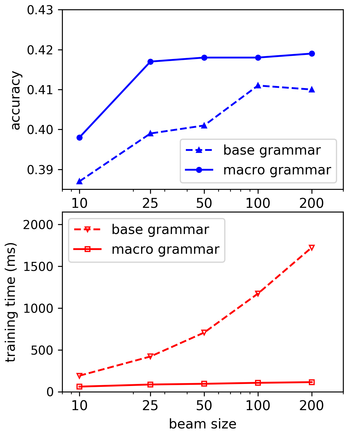
Figure 2(a) shows that for all beam sizes, training with the macro grammar is more efficient than training with the base grammar, and the speedup rate grows with the beam size. The test time accuracy of the macro grammar is robust to varying beam sizes as long as .
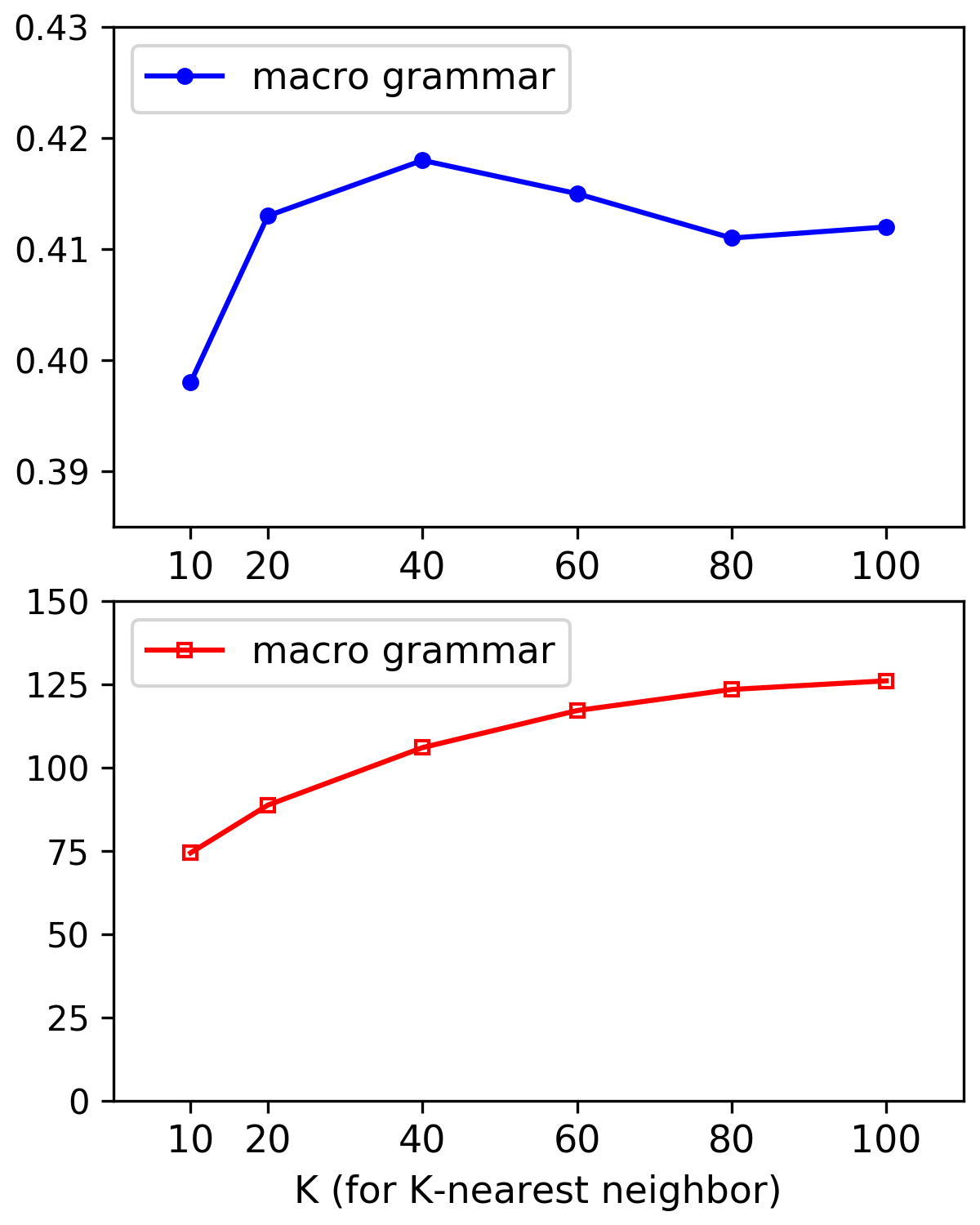
Figure 2(b) shows the influence of the neighbor size . A smaller neighborhood triggers fewer macro rules, leading to faster computation. The accuracy peaks at then decreases slightly for large . We conjecture that the smaller number of neighbors acts as a regularizer.
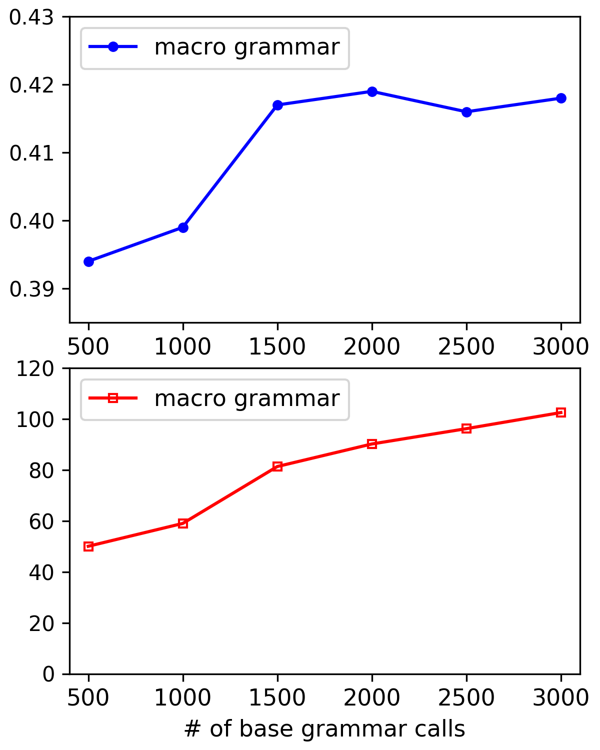
Figure 2(c) reports an experiment where we limit the number of fallback calls to the base grammar to . After the limit is reached, subsequent training examples that require fallback calls are simply skipped. This limit means that the macro grammar will get augmented at most times during training. We find that for small , the prediction accuracy grows with , implying that building a richer macro grammar improves the accuracy. For larger , however, the accuracies hardly change. According to the plot, a competitive macro grammar can be built by calling the base grammar on less than 15% of the training data.
Based on Figure 2, we can trade accuracy for speed by choosing smaller values of . With , and , the macro grammar achieves a slightly lower averaged development accuracy ( rather than ), but with an increased speedup of 15x (versus 11x) for training and 20x (versus 16x) for prediction.
5 Related work and discussion
A traditional semantic parser maps natural language phrases into partial logical forms and composes these partial logical forms into complete logical forms. Parsers define composition based on a grammar formalism such as Combinatory Categorial Grammar (CCG) Zettlemoyer and Collins (2007); Kwiatkowski et al. (2011); Kwiatkowski et al. (2013); Kushman and Barzilay (2013); Krishnamurthy and Kollar (2013), Synchronous CFG Wong and Mooney (2007), and CFG Kate and Mooney (2006); Chen and Mooney (2011); Berant et al. (2013); Desai et al. (2016), while others use the syntactic structure of the utterance to guide composition Poon and Domingos (2009); Reddy et al. (2016). Recent neural semantic parsers allow any sequence of logical tokens to be generated Dong and Lapata (2016); Jia and Liang (2016); Kociský et al. (2016); Neelakantan et al. (2016); Liang et al. (2017); Guu et al. (2017). The flexibility of these composition methods allows arbitrary logical forms to be generated, but at the cost of a vastly increased search space.
Whether we have annotated logical forms or not has dramatic implications on what type of approach will work. When logical forms are available, one can perform grammar induction to mine grammar rules without search (Kwiatkowski et al., 2010). When only annotated denotations are available, as in our setting, one must use a base grammar to define the output space of logical forms. Usually these base grammars come with many restrictions to guard against combinatorial explosion (Pasupat and Liang, 2015).
Previous work on higher-order unification for lexicon induction Kwiatkowski et al. (2010) using factored lexicons (Kwiatkowski et al., 2011) also learns logical form macros with an online algorithm. The result is a lexicon where each entry contains a logical form template and a set of possible phrases for triggering the template. In contrast, we have avoided binding grammar rules to particular phrases in order to handle lexical variations. Instead, we use a more flexible mechanism—holistic triggering—to determine which rules to fire. This allows us to generate logical forms for utterances containing unseen lexical paraphrases or where the triggering is spread throughout the sentence. For example, the question “Who is X, John or Y” can still trigger the correct macro extracted from the last example in Table 3 even when X and Y are unknown words.
Our macro grammars bears some resemblance to adaptor grammars Johnson et al. (2006) and fragment grammars O’Donnell (2011), which are also based on the idea of caching useful chunks of outputs. These generative approaches aim to solve the modeling problem of assigning higher probability mass to outputs that use reoccurring parts. In contrast, our learning algorithm uses caching as a way to constrain the search space for computational efficiency; the probabilities of the candidate outputs are assigned by a separate discriminative model. That said, the use of macro grammars does have a small positive modeling contribution, as it increases test accuracy from 42.7% to 43.7%.
An orthogonal approach for improving search efficiency is to adaptively choose which part of the search space to explore. For example, Berant and Liang (2015) uses imitation learning to strategically search for logical forms. Our holistic triggering method, which selects macro rules based on the similarity of input utterances, is related to the use of paraphrases Berant and Liang (2014); Fader et al. (2013) or string kernels Kate and Mooney (2006) to train semantic parsers. While the input similarity measure is critical for scoring logical forms in these previous works, we use the measure only to retrieve candidate rules, while scoring is done by a separate model. The retrieval bar means that our similarity metric can be quite crude.
6 Summary
We have presented a method for speeding up semantic parsing via macro grammars. The main source of efficiency is the decreased size of the logical form space. By performing beam search on a few macro rules associated with the -nearest neighbor utterances via holistic triggering, we have restricted the search space to semantically relevant logical forms. At the same time, we still maintain coverage over the base logical form space by occasionally falling back to the base grammar and using the consistent logical forms found to enrich the macro grammar. The higher efficiency allows us expand the base grammar without having to worry much about speed: our model achieves a state-of-the-art accuracy while also enjoying an order magnitude speedup.
Acknowledgements.
We gratefully acknowledge Tencent for their support on this project.
Reproducibility.
Code, data, and experiments for this paper are available on CodaLab platform: https://worksheets.codalab.org/worksheets/ 0x4d6dbfc5ec7f44a6a4da4ca2a9334d6e/.
References
- Artzi and Zettlemoyer (2013) Y. Artzi and L. Zettlemoyer. 2013. UW SPF: The University of Washington semantic parsing framework. arXiv preprint arXiv:1311.3011.
- Berant et al. (2013) J. Berant, A. Chou, R. Frostig, and P. Liang. 2013. Semantic parsing on Freebase from question-answer pairs. In Empirical Methods in Natural Language Processing (EMNLP).
- Berant and Liang (2014) J. Berant and P. Liang. 2014. Semantic parsing via paraphrasing. In Association for Computational Linguistics (ACL).
- Berant and Liang (2015) J. Berant and P. Liang. 2015. Imitation learning of agenda-based semantic parsers. Transactions of the Association for Computational Linguistics (TACL), 3:545–558.
- Chen and Mooney (2011) D. L. Chen and R. J. Mooney. 2011. Learning to interpret natural language navigation instructions from observations. In Association for the Advancement of Artificial Intelligence (AAAI), pages 859–865.
- Clarke et al. (2010) J. Clarke, D. Goldwasser, M. Chang, and D. Roth. 2010. Driving semantic parsing from the world’s response. In Computational Natural Language Learning (CoNLL), pages 18–27.
- Desai et al. (2016) A. Desai, S. Gulwani, V. Hingorani, N. Jain, A. Karkare, M. Marron, S. R, and S. Roy. 2016. Program synthesis using natural language. In International Conference on Software Engineering (ICSE), pages 345–356.
- Dong and Lapata (2016) L. Dong and M. Lapata. 2016. Language to logical form with neural attention. In Association for Computational Linguistics (ACL).
- Duchi et al. (2010) J. Duchi, E. Hazan, and Y. Singer. 2010. Adaptive subgradient methods for online learning and stochastic optimization. In Conference on Learning Theory (COLT).
- Fader et al. (2013) A. Fader, L. Zettlemoyer, and O. Etzioni. 2013. Paraphrase-driven learning for open question answering. In Association for Computational Linguistics (ACL).
- Guu et al. (2017) K. Guu, P. Pasupat, E. Z. Liu, and P. Liang. 2017. From language to programs: Bridging reinforcement learning and maximum marginal likelihood. In Association for Computational Linguistics (ACL).
- Haug et al. (2017) T. Haug, O. Ganea, and P. Grnarova. 2017. Neural multi-step reasoning for question answering on semi-structured tables. arXiv preprint arXiv:1702.06589.
- Indyk (2004) P. Indyk. 2004. Approximate nearest neighbor under edit distance via product metrics. In Symposium on Discrete Algorithms (SODA), pages 646–650.
- Jia and Liang (2016) R. Jia and P. Liang. 2016. Data recombination for neural semantic parsing. In Association for Computational Linguistics (ACL).
- Johnson et al. (2006) M. Johnson, T. Griffiths, and S. Goldwater. 2006. Adaptor grammars: A framework for specifying compositional nonparametric Bayesian models. In Advances in Neural Information Processing Systems (NIPS), pages 641–648.
- Kate and Mooney (2006) R. J. Kate and R. J. Mooney. 2006. Using string-kernels for learning semantic parsers. In International Conference on Computational Linguistics and Association for Computational Linguistics (COLING/ACL), pages 913–920.
- Kociský et al. (2016) T. Kociský, G. Melis, E. Grefenstette, C. Dyer, W. Ling, P. Blunsom, and K. M. Hermann. 2016. Semantic parsing with semi-supervised sequential autoencoders. In Empirical Methods in Natural Language Processing (EMNLP), pages 1078–1087.
- Krishnamurthy and Kollar (2013) J. Krishnamurthy and T. Kollar. 2013. Jointly learning to parse and perceive: Connecting natural language to the physical world. Transactions of the Association for Computational Linguistics (TACL), 1:193–206.
- Kushman and Barzilay (2013) N. Kushman and R. Barzilay. 2013. Using semantic unification to generate regular expressions from natural language. In Human Language Technology and North American Association for Computational Linguistics (HLT/NAACL), pages 826–836.
- Kwiatkowski et al. (2013) T. Kwiatkowski, E. Choi, Y. Artzi, and L. Zettlemoyer. 2013. Scaling semantic parsers with on-the-fly ontology matching. In Empirical Methods in Natural Language Processing (EMNLP).
- Kwiatkowski et al. (2010) T. Kwiatkowski, L. Zettlemoyer, S. Goldwater, and M. Steedman. 2010. Inducing probabilistic CCG grammars from logical form with higher-order unification. In Empirical Methods in Natural Language Processing (EMNLP), pages 1223–1233.
- Kwiatkowski et al. (2011) T. Kwiatkowski, L. Zettlemoyer, S. Goldwater, and M. Steedman. 2011. Lexical generalization in CCG grammar induction for semantic parsing. In Empirical Methods in Natural Language Processing (EMNLP), pages 1512–1523.
- Liang et al. (2017) C. Liang, J. Berant, Q. Le, and K. D. F. N. Lao. 2017. Neural symbolic machines: Learning semantic parsers on Freebase with weak supervision. In Association for Computational Linguistics (ACL).
- Liang (2013) P. Liang. 2013. Lambda dependency-based compositional semantics. arXiv preprint arXiv:1309.4408.
- Liang et al. (2011) P. Liang, M. I. Jordan, and D. Klein. 2011. Learning dependency-based compositional semantics. In Association for Computational Linguistics (ACL), pages 590–599.
- Neelakantan et al. (2016) A. Neelakantan, Q. V. Le, and I. Sutskever. 2016. Neural programmer: Inducing latent programs with gradient descent. In International Conference on Learning Representations (ICLR).
- O’Donnell (2011) T. J. O’Donnell. 2011. Productivity and Reuse in Language. Ph.D. thesis, Massachusetts Institute of Technology.
- Pasupat and Liang (2015) P. Pasupat and P. Liang. 2015. Compositional semantic parsing on semi-structured tables. In Association for Computational Linguistics (ACL).
- Poon and Domingos (2009) H. Poon and P. Domingos. 2009. Unsupervised semantic parsing. In Empirical Methods in Natural Language Processing (EMNLP).
- Reddy et al. (2016) S. Reddy, O. Täckström, M. Collins, T. Kwiatkowski, D. Das, M. Steedman, and M. Lapata. 2016. Transforming dependency structures to logical forms for semantic parsing. In Association for Computational Linguistics (ACL), pages 127–140.
- Wong and Mooney (2007) Y. W. Wong and R. J. Mooney. 2007. Learning synchronous grammars for semantic parsing with lambda calculus. In Association for Computational Linguistics (ACL), pages 960–967.
- Zettlemoyer and Collins (2007) L. S. Zettlemoyer and M. Collins. 2007. Online learning of relaxed CCG grammars for parsing to logical form. In Empirical Methods in Natural Language Processing and Computational Natural Language Learning (EMNLP/CoNLL), pages 678–687.
Supplementary material: macro analysis
The macro grammar extracts 123 macros from the WikiTableQuestions dataset, covering consistent logical forms for 75.6% examples. Let the frequency of a macro be defined as the number of highest-scoring consistent logical forms that it generates. We plot the frequency of all macros, sorted in decreasing order:
![[Uncaptioned image]](1707.07806v2/pyplot/template_freq.png)
As demonstrated by the plot, the top 20 macros cover 80% total frequency, and the top 34 macros cover 90% total frequency. It suggests that a small fraction of macros capture most examples’ consistent logical forms. By manually examining the top 34 macros, we find that 29 of them have explicit semantics. These macros correspond to abstract operations on the table, but when their slots are filled with concrete entities and relations33 3 A macro could have four categories of slots: • {Col#x} represents a column relation: Name, Rank, Venue, etc. • {Prop#x} represents a property relation: Number, Year, Date, etc. • {Compare#x} represents a comparative relation: >, <, >=, <=. • {Ent#x} represents an entity: Turkey, (number 2), (year 1998), etc. , they can be phrased in meaningful natural language utterances. Below, we interpret the meaning of each macro using examples from the WikiTableQuestions dataset:
- 1.
Macro: count({Col#1}.{Ent#2})
Description: the number of rows whose column {Col#1} matches {Ent#2}.
Example: how many records were set in Beijing ? - 2.
Macro: R[{Col#1}].{Col#2}.{Ent#3}
Description: select rows whose column {Col#2} matches {Ent#3}, then return all entities in column {Col#1}.
Example: what mine is in the town of Timmins? - 3.
Macro: R[{Prop#1}].R[{Col#2}].{Col#3}.{Ent#4}
Description: select rows whose column {Col#3} matches {Ent#4}, then return property {Prop#1} for all entities in column {Col#2}.
Example: what is the number of inhabitants living in Predeal? - 4.
Macro: count({Col#1}.{Prop#2}.{Compare#3}.{Ent#4})
Description: the number of rows satisfying some comparative constraint.
Example: how many directors served more than 3 years? - 5.
Macro: R[{Col#1}].argmax(Type.Row, R[.R[{Prop#2}].R[{Col#3}].])
Description: select the largest value in column {Col#3}, then for the associated row, return entities in column {Col#1}.
Example: which team scored the most goal? - 6.
Macro: R[{Col#1}].R[Next].{Col#1}.{Ent#2}
Description: return the entity right below {Ent#2}.
Example: who ranked right after Turkey? - 7.
Macro: R[{Col#1}].argmin(Type.Row, R[.R[{Prop#2}].R[Col#3].])
Description: select the smallest value in column {Col#3}, then for the associated row, return entities in column {Col#1}.
Example: which team scored the least goal? - 8.
Macro: R[{Col#1}].argmin(Type.Row, index)
Description: return column {Col#1} of the first row.
Example: which president is listed at the top of the chart ? - 9.
Macro: count({Col#1}.argmax(R[{Col#1}].Type.Row, R[.count({Col#1}.)]))
Description: N/A.
Example: N/A - 10.
Macro: count({Col#1}.argmin(R[{Col#1}].Type.Row, R[.count({Col#1}.)]))
Description: N/A.
Example: N/A - 11.
Macro: R[{Col#1}].argmax(Type.Row, index)
Description: return column {Col#1} of the last row.
Example: which president is listed at the bottom of the chart ? - 12.
Macro: R[{Col#1}].Next.argmin(R[{Col#1}].{Ent#2}, index)
Description: return the entity right above {Ent#2}.
Example: who is listed before Jon Taylor? - 13.
Macro: count(Type.Row)
Description: the total number of rows.
Example: what is the total number of teams? - 14.
Macro: argmax(R[{Col#1}].Type.Row, R[.count({Col#1}.)]))
Description: return the most frequent entity in column {Col#1}.
Example: which county has the most number of representatives? - 15.
Macro: sub(R[{Prop#1}].R[{Col#2}].{Col#3}.{Ent#4}, R[{Prop#1}].R[{Col#2}]
.{Col#3}.{Ent#5})
Description: Given two entities, calculate the difference for some property.
Example: how many more passengers flew to Los Angeles than to Saskatoon? - 16.
Macro: argmax(or({Ent#1}, {Ent#2}), R[.R[{Prop#3}].R[{Col#4}].{Col#5}.]))
Description: among two entities, return the one that is greater in some property.
Example: which is deeper, Lake Tuz or Lake Palas Tuzla? - 17.
Macro: R[{Col#1}].argmin({Col#1}.or({Ent#1}, {Ent#2}), index)
Description: N/A.
Example: N/A - 18.
Macro: R[{Col#1}].{Col#2}.{Prop#3}.{Compare#4}.{Ent#4}
Description: select rows whose property satisfies a comparative constraint, then return all entities in column {Col#1}.
Example: which artist have released at least 5 albums? - 19.
Macro: max(R[{Prop#1}].R[{Col#2}].Type.Row)
Description: return the maximum value in column {Col#2}.
Example: what is the top population on the chart? - 20.
Macro: R[{Prop#1}].R[{Col#2}].argmin(Type.Row, index)
Description: return a property in the first row’s column {Col#2}.
Example: what is the first year listed? - 21.
Macro: R[{Col#1}].argmin({Col#2}.{Prop#3}.{Compare#4}.{Ent#5}, index)
Description: select the first row that satisfies a comparative constraint, then return its column {Col#1}.
Example: what is the first creature after page 40? - 22.
Macro: R[{Col#1}].argmin({Col#2}.{Ent#3}, index)
Description: select the first row whose column {Col#2} matches entity {Ent#3}, then return its column {Col#1}.
Example: who is the top finisher from Poland? - 23.
Macro: R[{Col#1}].{Col#2}.{Prop#3}.{Ent#4}
Description: select rows whose column {Col#2} matches some property, then return all entities in column {Col#1}.
Example: who is the only one in 4th place? - 24.
Macro: R[{Prop#1}].R[{Col#2}].argmax(Type.Row, index)
Description: return a property of column {Col#2} of the first row.
Example: what is the first year listed? - 25.
- 26.
Macro: min(R[{Prop#1}].R[{Col#2}].Type.Row)
Description: return the minimum value in column {Col#2}.
Example: what is the least amount of laps completed? - 27.
Macro: R[{Col#1}].argmax({Col#2}.{Ent#3}, index)
Description: select the last row whose column {Col#2} matches entity {Ent#3}, then return its column {Col#1}.
Example: what was the last game created by Spicy Horse? - 28.
Macro: count({Col#1}.or({Ent#2}, {Ent#3}))
Description: the number of rows whose column {Col#1} matches either {Ent#2} or {Ent#3}.
Example: how many total medals did switzerland and france win? - 29.
Macro: R[{Prop#1}].R[{Col#2}].argmax(Type.Row, R[.R[{Prop#3}].R[{Col#4}].])
Description: select the largest value in column {Col#4}, then for the associated row, return a property of column {Col#2}.
Example: what year had the highest unemployment rate? - 30.
Macro: count({Col#1}.{Prop#2}.{Ent#3})
Description: the number of rows whose column {Col#1} matches a property {Ent#3}.
Example: how many people were born in 1976? - 31.
Macro: count(argmin(Type.Row, R[.R[{Prop#1}].R[Col#2].]))
Description: N/A.
Example: N/A - 32.
Macro: sub(count({Col#1}.{Ent#2}), count({Col#1}.{Ent#3}))
Description: Given two entities, calculate the difference of their frequencies in column {Col#1}.
Example: how many more games were released in 2005 than 2003? - 33.
Macro: R[{Prop#1}].R[{Col#2}].argmax(Type.Row, R[.R[{Prop#1}].R[Col#3].])
Description: same as macro 29, but with an additional constraint that the two properties in the logical form must be equal.
Example: which game number has the most attendance? - 34.
Macro: R[{Col#1}].R[Next].argmin(Type.Row, index)
Description: N/A.
Example: N/A