Mode-Coupling Theory for Active Brownian Particles

The collective dynamics of self-propelled particles and the related behavior of dense suspensions of microswimmers have received an increasing amount of attention in the past few years. The physical principles of this dynamics are relevant for many biophysical questions. For example, mechanisms at work in wound healing (tissue repair) have been likened to the collective dynamics found in model microswimmer systems [1, 2, 3, 4, 5] . The collective dynamics of bacteria colonies [6], as well as the dynamics of the cell cytoskeleton show slow dynamics typically associated with that arising from crowding effects at high densities and associated glass-like slowing down [7, 8, 9].

Colloidal self-propelled particles provide paradigmatic model systems to study the qualitative effects of swimming, and more generically the generic features of a broad class of intrinsically non-equilibrium matter. In experiment, self-phoretic Brownian particles provide a good realization of this model. Half-capped “Janus particles” provide a surface-mediated mechanism to convert energy provided by light fields or chemical fuel into directed motion, superimposed on the Brownian translational and rotational diffusion of passive colloids [10, 11, 12, 13, 14].

One of the simplest theoretical models in this context is that of active Brownian particles (ABP) [15, 16]. These are orientable colloidal particles that undergo “passive” translational and rotational Brownian motion (ignoring hydrodynamic interactions in the following), and in addition an “active” drift along a body-fixed orientation axis due to intrinsic self-propulsion forces. In two spatial dimensions, particles are described by their positions $\vec{r}_{i}$ and orientation angles $\theta_{i}$ with respect to a fixed direction in space. Here, $i=1,\ldots N$ labels the particles. The equations of motion read, in the case of spherically symmetric interaction forces,

where $\vec{o}(\theta)=(\cos\theta,\sin\theta)^{T}$ is the orientation vector. We will abbreviate $\vec{o}_{i}=\vec{o}(\theta_{i})$. The elements of $dW$ are independent Wiener processes, and the $\vec{F}_{i}$ are the interaction forces. The friction coefficient $\zeta=1/\beta D_{t}$ is taken to obey the fluctuation-dissipation theorem for the translational Brownian motion of the passive-particle system, with inverse temperature $\beta$. The key parameters characterizing the dynamics of a single spherical ABP are $D_{t}$, $D_{r}$, and $v_{0}$: the translational short-time diffusion coefficient, the rotational diffusion coefficient, and the self-propulsion velocity. Although for a passive colloid, $D_{r}$ and $D_{t}$ are coupled due to the hydrodynamics of the solvent, for spherical ABP it makes sense to treat $D_{r}$ as an independent model parameter. Different self-propulsion mechanisms may impose different persistence effects on the orientation, and to some extent these can be captured by varying $D_{r}$ [17].

We focus on spherical ABP with strongly repulsive interactions, modeled by the equilibrium structure of a hard-sphere suspension. At high densities, such systems (with suitable size polydispersity) are known from simulation to form glasses [18, 19, 20], as do related active-particle models [21, 22, 23, 24, 25, 16, 5].

The theory of ABP has been extensively studied at low and moderate densities [26, 27, 28, 29, 30]. At large time scales, $D_{r}t\gg 1$, an “effective-diffusion limit” can be performed to map the dynamics of the dilute system onto Brownian motion with an effective diffusion coefficient: $D_{\text{eff}}=D_{t}+D_{\text{act}}=D_{t}(1+\mathit{Pe}/2)$, where $\mathit{Pe}=v_{0}^{2}/D_{r}D_{t}$ defines the relevant Péclet number and $D_{\text{act}}=v_{0}^{2}/2D_{r}$ is an activity-induced diffusivity. Accounting for this enhancement of diffusivity, many properties of dilute ABP suspensions and their phase behavior can be explained [26, 27]. The mapping however requires that all relevant length scales in the problem are large compared to the average swim length $\ell_{p}=v_{0}/D_{r}$, and that one probes the system on length scales larger than that [28, 29].

The high-density dynamics of ABP is less well explored. To describe glassy behavior of active systems, theories of the glass transition have been extended from the passive near-equilibrium case to include self propulsion [31, 32, 33, 24, 34, 35, 36], using various different models and approximations. One particular reference point for the passive Brownian system is the mode-coupling theory of the glass transition (MCT), both in 3D [37] and in 2D [38]. MCT has been extended to deal with spherical ABP in the effective-diffusion limit [32]. In this limit, the equations of motion, Eq. (1), can be formally reduced to eliminate the orientation angles $\theta_{i}$ as explicit variables, in a procedure akin to the well-known reduction of the phase-space Langevin equation to the configuration-space Brownan dynamics. One obtains $d\vec{r}_{i}=\vec{F}_{i}/\zeta_{\text{eff}}+\sqrt{2D_{t}}\,d\vec{W}_{i}$ where $\zeta_{\text{eff}}$ is an effective friction coefficient. The resulting MCT takes the same form as the passive-equilibrium theory, with an activity-dependent prefactor in the memory kernel that reflects the non-equilibrium nature of the system through a violation of the fluctuation-dissipation theorem, $\zeta_{\text{eff}}\neq 1/\beta D_{t}$. Consequently, activity enters this theory only through the Péclet number $\mathit{Pe}$. This MCT approach extends easily to mixtures of active and passive particles [39]. It predicts a shift of the glass transition to higher densities, in qualitative agreement with simulation results.

However, the approach to a glass transition implies transient caging of particles on a length scale $\ell_{c}\sim 0.1\sigma$ (where $\sigma$ is a typical particle size), over increasingly long times. It is not evident that the effective-diffusion approach remains valid as the condition $\ell_{c}<\ell_{p}$ is easily violated for typical swim speeds used in simulation and experiment. This calls for a theoretical treatment that starts directly from Eq. (1), rather than from a further reduced description of the dynamics.

Besides the ABP, the best studied model of active particles to date is the one proposed by Berthier, Szamel, and coworkers [24, 34], that of active Ornstein-Uhlenbeck particles (AOUP). Here, particles are described by their positions and an activity vector that represents the swimming direction and evolves according to an Ornstein-Uhlenbeck process providing colored noise for the evolution of the positions. The model thus belongs to a class where activity is modeled as leading to a persistent random walk of the particles [40, 41, 42]. This and related models have been studied in simulation [22, 43, 23, 25, 44] as the extension of paradigmatic passive glass formers to the non-equilibrium regime. A theoretical treatment based on MCT was established [34], under the simplifying assumption that the particle positions evolve on a time scale larger than the time scale governing the evolution of the activity vector. This is not unlike the effective-diffusion approximation made in previous studies of high-density ABP systems. Predictions of the AOUP-MCT have been tested in computer simulation [44]. In the “athermal” case where activity is the sole driving force, the glass transition was found to depend non-monotonically on the activity strength [34]. This appears to be different for “thermal” ABP, according to present simulation results. Thus the connection among different models of active colloidal systems remains to be studied in more detail.

In this paper, we develop a MCT of spherical ABP that treats both the positional and orientational degrees of freedom on equal footing. This avoids the reduction to a near-equilibrium or an effective-diffusion description, and allows to study the qualitative effects of self-propulsion of various persistence lengths in the high-density regime. In particular it allows to study the limits $D_{r}\to 0$ and $D_{r}\to\infty$ as interesting reference cases [45] that provide valuable insight into the mechanisms by which swimming modifies the caging dynamics; Our approach is based on the integration-through transients (ITT) formalism as a formal approach to deal with the self-propulsion force as an arbitrarily strong perturbation of the passive-equilibrium dynamics.

The paper is organized as follows: in Sec. II we derive the MCT for two-dimensional spherical ABP, including rotational degrees of freedom. Section III shows numerical results for the dynamical density correlation functions close to the glass transition; Sec. IV is devoted to a discussion of the dependence of the glass-transition point on activity. Section V concludes.

The statistical information of the dynamics of a system composed of $N$ spherical ABP is encoded in the Smoluchowski equation for the configuration-space distribution function $p(\Gamma,t)$, i.e., the probability density that corresponds to the Markov process described by the stochastic differential equations Eq. (1). Here $\Gamma=(\Gamma_{r},\Gamma_{\theta})=(\vec{r}_{1},\ldots,\vec{r}_{N},\theta_{1},\ldots,\theta_{N})$ labels points in configuration space. There holds $\partial_{t}p(\Gamma,t)=\smol(\Gamma)p(\Gamma,t)$ with the Smoluchowski operator

where $\dsmol(v_{0})=-v_{0}\sum_{j}\vec{\nabla}_{j}\cdot\vec{o}(\theta_{j})$ is the term that represents the active motion. The interaction forces are assumed to follow from a spherically symmetric interaction potential, $\vec{F}_{j}=-\vec{\nabla}_{j}U(\Gamma_{r})$.

Equation (2) for $v_{0}=0$ describes the passive Brownian system. It admits the equilibrium solution $p_{\text{eq}}(\Gamma_{r})\propto\exp[-\beta U(\Gamma_{r})]$. The integration-through transients (ITT) formalism expresses averages of observables in the non-equilibrium system through history integrals involving transient correlation functions, i.e., correlation functions that contain the full non-equilibrium time evolution but are taken with the equilibrium distribution function. The starting point of ITT is the identity $\exp[\smol t]=1+\int_{0}^{t}dt^{\prime}\exp[\smol t^{\prime}]\smol$. Using this identity to rewrite $p(t)=\exp[\smol t]p(0)$, and assuming that for $t=0$ the system starts in equilibrium, one gets a generalized Green-Kubo formula for any observable $A$. For the special case of the spherical ABP system,

The desire to evaluate expressions like this prompts the development of a theory of transient correlation functions. In the following, we will drop the subscript “eq” and implicitly perform all averages over the equilibrium distribution.

The collective motion of the particles is described by the local density fluctuations, $\varrho(\vec{r},\theta)=\sum_{j=1}^{N}\delta(\vec{r}-\vec{r}_{j})\delta(\theta-\theta_{j})$, respectively their Fourier transform

with integer angular indices $l=-\infty,\ldots,\infty$. We assume the system to remain in a homogeneous, translationally invariant and isotropic state. Then, the equilibrium static structure factor matrix depends on the wave vector only through $q=|\vec{q}|$,

Also the two-point density correlation functions are diagonal in wave-vector space under these conditions. Since the interaction potential is spherically symmetric, the matrix $\boldsymbol{S}(q)$ takes the simple form

i.e., it is the unit matrix with its $(00)$ element replaced by $S_{q}$, the usual static structure factor of the equilibrium system of spherical particles.

The time-dependent transient density correlation functions are defined as

Here, the adjoint (or backward) Smoluchowski operator provides the temporal evolution,

We use the convention that this operator acts to everything on its right, but not on the distribution function itself. There holds $\boldsymbol{S}(\vec{q},0)=\boldsymbol{S}(q)$. The normalized correlator is defined by $\boldsymbol{\Phi}(\vec{q},t)=\boldsymbol{S}(\vec{q},t)\cdot\boldsymbol{S}^{-1}(q)$.

The correlation functions are defined in a specific laboratory frame of reference, with respect to which particle orientations are measured. For this reason, the correlation functions depend a priori on the direction of the wave vector $\vec{q}$. However, there hold simple transformation rules to transform the correlators to a rotated reference frame. Consider a rotation around an angle $\alpha$, $\vec{r}\mapsto\vec{r}^{\,\prime}=\boldsymbol{D}(\alpha)\cdot\vec{r}$ and $\theta\mapsto\theta^{\prime}=\theta+\alpha$, witth $\boldsymbol{D}\cdot\boldsymbol{D}^{T}=1$ a rotation matrix. This changes $\mathit{\delta\varrho}_{l}(\vec{q})\mapsto\mathit{\delta\varrho}_{l}(\vec{q}^{\,\prime})\exp[il\alpha]$ where $\vec{q}^{\,\prime}=\boldsymbol{D}\cdot\vec{q}$. The transformation is thus given by a unitary representation $\boldsymbol{u}(\alpha)$ of the orientation group $\mathit{SO}(1)$, given by $u_{ll^{\prime}}=\exp[-il\alpha]\delta_{ll^{\prime}}$. (There holds $\boldsymbol{u}(\alpha)\cdot\boldsymbol{u}(\beta)=\boldsymbol{u}(\alpha+\beta)$, $\boldsymbol{u}(\alpha)\boldsymbol{u}^{\dagger}(\alpha)=\boldsymbol{1}$, $\boldsymbol{u}(0)=\boldsymbol{1}$, and $\boldsymbol{u}(\alpha+2\pi)=\boldsymbol{u}(\alpha)$, as well as $\det\boldsymbol{u}=1$.) One easily shows that the Smoluchowski operator itself is invariant under rotation, $\smoluch(\Gamma)=\smoluch^{\prime}(\Gamma^{\prime})$, seperately in all its terms. (To see this, recall $\vec{\partial}^{\,\prime}\cdot\vec{o}(\theta^{\prime})=(\boldsymbol{D}^{-1}\cdot\vec{\partial})\cdot\vec{o}(\theta+\alpha)=\vec{\partial}\cdot\boldsymbol{D}\cdot\vec{o}(\theta+\alpha)=\vec{\partial}\cdot\vec{o}(\theta)$. Under rotation, the equilibrium distribution function remains invariant, and thus one obtains the transformation rule

We will make use of this relation to restrict the discussion of the correlation functions to wave vectors aligned with a particular spatial direction, chosen by $\vec{q}=q\vec{e}_{y}$. Note that Eq. (9) confirms that $S_{00}(q,t)$ is in fact invariant under rotations.

An equation of motion for $\boldsymbol{S}(\vec{q},t)$ can be derived using the Mori-Zwanzig projection operator formalism. Introduce the projection operator onto density fluctuations,

and set $\projQ=1-\projP$. One now writes $\partial_{t}\exp[\adsmol t]=\adsmol(\projP+\projQ)\exp[\adsmol t]$ and rewrites the second term using the Dyson decomposition

to obtain

where $\boldsymbol{\omega}(\vec{q})$ generalizes the collective diffusion matrix,

writing $\vec{q}=q(\cos\vartheta_{q},\sin\vartheta_{q})^{T}$. The memory kernel $\boldsymbol{K}(\vec{q},t)$ is given by

It describes the renormalization of the diffusion matrix due to many-body interactions.

For small density, $\rho=N/V\to 0$ (where $V$ is the system volume), one can drop the memory kernel in Eq. (12). The formal solution, $\boldsymbol{S}(\vec{q},t)=\exp[-\boldsymbol{\omega}(\vec{q})t]$, reproduces the exact solution as discussed in 3D [30].

The slowing down of the dynamics close to a glass transition is driven by slow positional density fluctuations. This suggests to split the time-evolution operator, $\smol=\smol_{T}(D_{t},v_{0})+\smol_{R}(D_{r})$. The matrix elements of the translational and rotational parts will be written as $\boldsymbol{\omega}(\vec{q})=\boldsymbol{\omega}_{T}(\vec{q})+\boldsymbol{\omega}_{R}(\vec{q})$, i.e., $\omega_{R,ll^{\prime}}(\vec{q})=l^{2}D_{r}\delta_{ll^{\prime}}$. Correspondingly, we decompose the memory kernel into four contributions, $\boldsymbol{K}(t)=\boldsymbol{K}^{TT}(t)+\boldsymbol{K}^{TR}(t)+\boldsymbol{K}^{RT}(t)+\boldsymbol{K}^{RR}(t)$, given by replacing the operators $\adsmol$ appearing to the right and to the left of the reduced propagator in Eq. (14) by their decompositions.

Since in our model of spherical ABP, the rotational degrees of freedom never slow down, all contributions to the memory kernel involving $\smol_{R}^{\dagger}$ vanish, and there holds $\boldsymbol{K}(t)=\boldsymbol{K}^{TT}(t)$. (This is also explicitly checked in a mode-coupling approximation.)

To describe slow dynamics arising from a coupling of translational modes, we follow the standard procedure of MCT and rewrite the diffusion kernel $\boldsymbol{K}^{TT}(t)$ in terms of a friction kernel. To do so, introduce a further projector,

where $\boldsymbol{\psi}(\vec{q})=\boldsymbol{\omega}_{T}^{-1}(\vec{q})$ normalizes the projector. We now decompose the propagator that appears in Eq. (14) according to

This results in

where we have defined the friction memory kernel

Note that $\boldsymbol{M}(\vec{q},t)$ and $\boldsymbol{K}^{TT}(\vec{q},t)$ only differ in their time evolution. In the context of passive Brownian particles, the operator appearing in Eq. (18) is also referred to as the one-particle irreducible Smoluchowski operator .

Equations (12) and (17) can be combined to a time-evolution equation for the density correlation functions that is a suitable starting point for approximations of the slow dynamics arising from the slow evolution of positional density fluctuations,

Equations (19) are the starting point of mode-coupling approximations for glassy dynamics. Setting $v_{0}=0$, the matrices all become diagonal (since $\smol^{\dagger}_{T}$ does not mix translational and rotational degrees of freedom in this case), and one recovers for $S_{00}(q,t)$ the standard Mori-Zwanzig equation used to derive MCT for Brownian spherical particles.

Rotational diffusion appears in Eqs. (19) in the form of a “hopping term” in the MCT language, viz. the last term under the integral in Eq. (19a). The original MCT only contains a convolution of the memory kernel with the time derivative of the density correlation function, viz. the first term under the integral in Eq. (19a). In this form the equations allow for an ideal glass transition: there exist solutions with a non-zero long-time limit $\lim_{t\to\infty}\boldsymbol{S}(\vec{q},t)=\boldsymbol{F}(\vec{q})\neq\boldsymbol{0}$. The presence of the density correlator itself in the convolution integral for $l\neq 0$ causes the corresponding solutions to ultimately decay exponentially: since rotation remains unhindered even in the dense system, the associated density fluctuations will decay on a time scale $1/(l^{2}D_{r})$. Note that Eq. (19) still allows for an ideal glass transition for all transient density correlation functions $S_{ll^{\prime}}(\vec{q},t)$ with $l=0$.

The MCT approximation now consists of two intertwined steps: first the fluctuating forces $\projQ\smol^{\dagger}_{T}\mathit{\delta\varrho}_{l}(\vec{q})$ that appear in $\boldsymbol{M}(\vec{q},t)$ are replaced by their overlap with density-fluctuation pairs. Using the short-hand notation $\mathit{\delta\varrho}_{1}\equiv\mathit{\delta\varrho}_{l_{1}}(\vec{q}_{1})$, one introduces the pair-density projector

with a suitable normalization matrix $\chi$. Second, the resulting dynamical four-point correlation functions that involve the reduced dynamics are replaced by the product of two-point correlation functions propagated by the full dynamics,

together with a consistent approximation of $\chi$. For a detailed derivation of the MCT expression for the memory kernel, we refer to Appendix A. One gets

The vertices are given by $\mathcal{V}^{\dagger}_{ll_{1}l_{2}}(\vec{q},\vec{k},\vec{p})=\sum_{m}(\boldsymbol{\omega}_{T}^{-1}(\vec{q}))_{lm}\mathcal{W}^{\dagger}_{ml_{1}l_{2}}(\vec{q},\vec{k},\vec{p})$ and $\mathcal{V}_{ll_{1}l_{2}}(\vec{q},\vec{k},\vec{p})=\sum_{m}(\boldsymbol{\omega}_{T}^{-1})_{lm}(\vec{q})\mathcal{W}_{ml_{1}l_{2}}(\vec{q},\vec{k},\vec{p})$, with

where we have defined $\tilde{S}_{ll^{\prime}}(k)=S_{l^{\prime}l^{\prime}}^{-1}(k)S_{l,l}(k)$. The left vertex is the same as in equilibrium,

It differs from $\mathcal{W}^{\dagger}$ because the time-evolution operator $\adsmol$ is not self-adjoint with respect to the scalar product defined by the equilibrium averages.

For $v_{0}=0$, these equations reduce to the equilibrium MCT expressions. In particular, in this case $\mathcal{V}$ and $\mathcal{V}^{\dagger}$ do no longer explicitly depend on $D_{t}$. In the active case, $v_{0}\neq 0$, one readily checks that the explicit dependence on $D_{t}$ still cancels in the memory kernel if the self-propulsion velocity is expressed in terms of a Péclet number $\mathit{Pe}_{t}=v_{0}\sigma/D_{t}$, where $\sigma$ is a typical particle diameter. There is no dependence on $D_{r}$ in the memory kernel, and therefore the Péclet number $\mathit{Pe}=v_{0}^{2}/D_{t}D_{r}$ does not assume the natural role in determining the MCT dynamics that is has for the low-density system.

The MCT approximation preserves the transformation properties of the correlation functions under rotation, Eq. (9). In fact, the same transformation law is required for all the quantities that appear in the Mori-Zwanzig equations, Eq. (12) or (19a). In particular, $\boldsymbol{\omega}(\vec{q})\mapsto\boldsymbol{u}(\alpha)\cdot\boldsymbol{\omega}(\vec{q}^{\,\prime}\cdot\boldsymbol{\omega}^{\dagger}(\alpha)$ is easily checked. For the MCT vertices, a straightforward calculation shows $\mathcal{W}_{ll_{1}l_{2}}^{\dagger}(\vec{q},\vec{k},\vec{p})\mapsto\mathcal{W}_{l^{\prime}l_{1}^{\prime}l_{2}^{\prime}}^{\dagger}(\vec{q}^{\,\prime},\vec{k}^{\,\prime},\vec{p}^{\,\prime})u_{ll^{\prime}}(\alpha)u^{\dagger}_{l_{1}^{\prime}l_{1}}(\alpha)u^{\dagger}_{l_{2}^{\prime}l_{2}}(\alpha)$ and equivalently for $\mathcal{W}_{ll_{1}l_{2}}(\vec{q},\vec{k},\vec{p})$, i.e., all terms that appear in the MCT expression for $\boldsymbol{m}(\vec{q},t)$ transform like tensors.

The fact that the MCT approximation preserves the transformation properties of the correlation functions under rotation, allows us to pick a coordinate system where $\vec{q}$ is aligned along a coordinate axis, $\vec{q}=q\vec{e}_{y}$, say. By using the unitary transformation property, all correlation functions entering the MCT memory kernel can be rewritten in terms of those evaluated with $\vec{q}$ aligned along the same axis. For completeneess, this form of the MCT equations is documented in Appendix B. This allows to reduce the numerical calculation to wave vectors along a single spatial axis.

The MCT equations have been solved numerically on a grid of $128$ wave numbers equally spaced up to $|\vec{q}|\leq Q$ with $Q\sigma=50$. For the angular indices, a cutoff $|l|\leq L$ with $L=1$ has been introduced. Some results have been checked with $L=2$, but the effects were minor. The presence of the “hopping” term with its singular structure (imposed by $\omega_{R,00}=0$) poses a numerical problem at long times. We have developed an extension of the standard algorithm that is usually employed to solve MCT equations, and that we outline in Appendix C.

To determine the MCT vertex, the equilibrium static structure factor is needed. In odd dimensions, the Percus-Yevick approximation provides a reasonably accurate analytical expression. However, in even dimensions, no such analytical solution is known. We use the Baus-Colot expression for $S(q)$ that is known to be close to simulation data.

We fix units of length and time by the particle diameter $\sigma=1$ and the translational free-diffusion time $\sigma^{2}/D_{t}=1$. Densities are reported as packing fractions, $\phi=(\pi/4)\rho\sigma^{2}$. With the chosen parameters, we obtain a glass transition in the passive hard-disk system at a critical packing fraction $\phi_{c}\approx 0.7207$; this is in reasonable agreement with the value reported in earlier work [38]. In comparison to this work, we have improved the numerical evaluation of the wave-vector integrals appearing in the MCT memory kernel; see Appendix B for details.

Exemplary MCT results for the density correlation functions $\Phi_{00}(\vec{q},t)$ are shown in Fig. 1. A wave number $q\sigma=8$ in the vicinity of the main peak of the equilibrium $S(q)$ was chosen. The density correlation functions show the qualitative features expected for dense colloidal suspensions nearing dynamical arrest: after an initial relaxation, a plateau emerges at high densities that extends over an increasingly large intermediate-time window as the density is increased. The final relaxation from this plateau to zero is termed structural relaxation, and its characteristic time increases strongly with increasing density. At the highest densities shown, structural relaxation becomes ineffective and is not seen over the full time window accessible to the numerical solution scheme. Hence, $\lim_{t\to\infty}\Phi_{00}(\vec{q},t)=F_{00}(\vec{q})>0$. This non-zero positive non-ergodicity parameter signals the appearance of an ideal glass.

With increasing self-propulsion velocity $v_{0}$, the dynamics speeds up, as shown in the upper panel of the figure. This is qualitatively expected, since self-propulsion renders the particle motion more vivid, and this opposes the slow dynamics. This result is also qualitatively consistent with earlier Brownian-dynamics (BD) simulation studies of three-dimensional ABP [18]. (Note that there, stationary-state non-equilibrium correlation functions were reported, while the central object of our MCT are the transient non-equilibrium, equilibrium-averaged correlation functions.)

For small enough self-propulsion velocity, the glass remains stable at sufficiently high density. This is exemplified by the lower panel of Fig. 1, where curves for constant $v_{0}=0.5\,D_{t}/\sigma$ are shown. At the highest packing fractions shown, no sign of structural relaxation is seen in the numerical results over the time window covered in the figure.

Hence, for small enough but finite $v_{0}$ MCT predicts an ideal “active glass”. As the lower panel of Fig. 1 demonstrates, the signature of the transition to this active glass is qualitatively as for the passive ideal glass: with increasing density at fixed $v_{0}$, structural relaxation dramatically slows down until it completely arrests at the transition density $\phi_{c}$. Further increasing the density causes the nonergodicity parameter to increase. The ideal glass transition is discontinuous in the sense that the long-time limit of the density correlation functions jumps from zero in the liquid ($\phi<\phi_{c}$) to a finite value at $\phi_{c}$.

These results suggest that there is a line of ideal glass transitions $(\phi_{c},v_{0}^{c})$ in the density–self-propulsion plane. This line shifts to increasing density with increasing $v_{0}$. Qualitatively, this result has been derived in earlier extensions of MCT that do not account for orientational degrees of freedom explicitly [32].

With the present approach, the influence of the rotational diffusion coefficent on the dynamics can be studied. Figure 2 exemplifies the effects of increasing $D_{r}$ on the dynamics at fixed self-propulsion velocity. Keeping the other parameters fixed, an increase in $D_{r}$ leads to a slowing down of the structural-relaxation dynamics. Qualitatively, this is expected from the argument that faster reorientation of the individual particles causes the self propulsion to be less effective in melting nearest neighbor cages, since for the latter process a certain persistence of the self-propulsion force in a specific direction needs to be maintained. The slowing down with increasing $D_{r}$ is more pronounced at higher densities: while at $\phi=0.7$, the final relaxation of the curves shown in Fig. 2 spreads out by about a factor $2$, the same change in $D_{r}$ causes the structural-relaxation time to change by a factor of about $10$ at $\phi=0.718$.

The structural relaxation dynamics of the weakly active system shows the same qualitative features as they are known from the passive system. In particular, the structural relaxation process can be well described by a stretched-exponential function in time for the cases shown in Figs. 1 and 2. It is known from the passive system, that density fluctuations with wavelengths comparable to the particle size govern the slow dynamics.

For the active system, the persistence of self propulsion sets another length scale, $\ell_{p}=v_{0}/D_{r}$. This suggests to discuss the effect of density fluctuations on length scales much larger, comparable to, and much smaller than the persistence length. Let us introduce a rescaled wave number $\tilde{q}=q\ell_{p}/(2\pi)$. The low-density dynamics of ABP exhibits three distinct regimes [30]: for $\tilde{q}\ll 1$ probe the dynamics on length scales large compared to $\ell_{p}$, and hence see diffusive relaxation with a diffusion coefficient $D_{\text{eff}}$. For small length scales, probed by $\tilde{q}\gg 1$, the initial Brownian passive diffusion of the ABP is seen, and the density correlators decay diffusively, with diffusion coefficient $D_{t}$. Activity causes an intermediate regime $\tilde{q}\approx 1$ to appear, where the persistent swimming motion affects the relaxation of density fluctuations. Over the length scales probed in this regime, particles swim in a fixed direction and cause density fluctuations to decay in a damped-oscillatory fashion, leading to pronounced “undershoots” in the final relaxation.

The influence of high-density interactions on this single-particle picture is examined in Fig. 3. Here, state points close to the glass transition were chosen and to make connection to the low-density theory, different activities along a cut with constant Péclet number, $\mathit{Pe}=32$, are shown. The panels of Fig. 3 correspond to increasing self-propulsion velocity (from top left to bottom right), and at fixed $\mathit{Pe}$, these correspond to decreasing persistence lengths. Essentially, the low-density scenario is recovered for the case $\ell_{p}<\sigma$, i.e., for large self-propulsion velocity. There, structural arrest is effectively destroyed by active driving, and the correlation functions decay on a time scale $\tau_{\text{rot}}=1/D_{r}$, showing oscillations around $\tilde{q}\approx 1$ (cf. lower panels of Fig. 3).

For large persistence length, $\ell_{p}\gg\sigma$, the top panels of Fig. 3 demonstrate that the low-density scenario is absent. Here, all correlation functions decay without oscillations. This result can be interpreted as showing that once the interparticle length scale becomes smaller than $\ell_{p}$, density fluctuations can no longer be translated by persistent motion; they relax by the combination of diffusion and activity-modified structural interactions. Coincidently, for the $\ell_{p}\gg\sigma$ cases shown in Fig. 3, the intermediate-time plateau of structural relaxation begins to emerge at large $\tilde{q}$ (corresponding to intermediate $q\sigma$).

The appearance of oscillatory relaxation in the density correlation functions of a Brownian system is a clear signature of non-equilibrium dynamics. Recall that the equilibrium Smoluchowski operator $\smol_{\text{eq}}$ is negative semi-definite, i.e., it has non-positive real eigenvalues only. As a result, the corresponding auto-correlation functions are completely monotone functions: they can be written as superpositions of purely relaxing exponential functions with positive weights. This is a feature that is preserved under the MCT approximation.

To highlight the dynamics of the reorientational degrees of freedom, we show in Fig. 4 the matrix elements of $\Phi_{ll^{\prime}}(\vec{q},t)$ for $|l|\leq 1$. Only positive $l,l^{\prime}$ are shown for siplicity, and the case $l=l^{\prime}=0$ is repeated from above for reference. The $(ll^{\prime})=(11)$ correlator reflects the decay of orientational order. It decays on the time scale $\tau_{\text{rot}}=\sigma/D_{r}$, with a final exponential relaxation. This is expected since in the spherical ABP model, rotation is not influenced by the packing of particles. Note that the decay of $\Phi_{11}(\vec{q},t)$ is not purely exponential; even at low densities and without self propulsion, $\Phi_{11}(\vec{q},t)\sim\exp[-q^{2}D_{t}t]\exp[-D_{r}t]$. In general, the $(ll^{\prime})=(11)$ correlator inherits a signature of the translational motion for $t\ll\tau_{\text{rot}}$, which is cut off by an exponential decay at $t\sim\tau_{\text{rot}}$.

The off-diagonal elements $(ll^{\prime})=(01)$ and $(10)$ of the transient density correlation function behave different from each other. In equilibrium, one expects the matrix of correlation functions to be symmetric (as is the case for example in the MCT developed for Newtonian non-spherical particles [46, 47, 48]). This symmetry is lost in the present theory because the time-evolution operator is not self-adjoint with respect to the equilibrium-weighted scalar product.

The off-diagonal elements vanish with $v_{0}\to 0$, as expected from the structure of the Smoluchowski equation for spherical ABP. Interestingly, the correlation function $\Phi_{01}(\vec{q},t)$ shows non-trivial slow dynamics that is coupled to the slow dynamics of the positional-density correlator $\Phi_{00}(\vec{q},t)$. In particular it displays structural relaxation that slows down beyond the time scale $\tau_{r}$ over which orientational order decays. The correlation function $\Phi_{10}(\vec{q},t)$ instead decays on the reorientational time scale $\tau_{\text{rot}}$.

This observation can be rationalized by the peculiar structure of the equations of motion of spherical ABP: orientations influence the slow dynamics of the positions, but not vice versa. Thus, the evolution of positional density fluctuations, $\exp[\smol^{\dagger}t]\mathit{\delta\varrho}_{0}(\vec{q})$, will not be detectable in the subspace spanned by the orientations, $\mathit{\delta\varrho}_{1}^{*}(\vec{q})$, for times $t\gg\tau_{\text{rot}}$. On the other hand, the impact of the time-evolved initial polar order, $\exp[\smol^{\dagger}t]\mathit{\delta\varrho}_{1}(\vec{q})$, on the positional density fluctuations of the system, $\mathit{\delta\varrho}_{0}^{*}(\vec{q})$, persists until the time of overall structural relaxation, hence $S_{01}(\vec{q},t)=\langle\mathit{\delta\varrho}_{0}^{*}(\vec{q})\exp[\smol^{\dagger}t]\mathit{\delta\varrho}_{1}(\vec{q})\rangle$ decays as slow as $S_{00}(\vec{q},t)$.

The usual quantification of the slow dynamics is in terms of the structural relaxation time $\tau$. Following the operational defition used in many studies of glassy dynamics, we define $\tau$ as the time where the density-correlation function has decayed to $1\%$ of its initial value, $\Phi_{00}(\vec{q},\tau)=0.01$.

Results for $\tau(\varphi)$ for a fixed self-propulsion velocity are shown in Fig. 5. As anticipated from the discussion above, the structural relaxation time strongly increases with increasing packing fraction, in a power-law fashion that is the hallmark of the approach to the MCT glass transition. At fixed $v_{0}$, increasing $D_{r}$ increases the structural relaxation time. For $D_{r}\to\infty$, the $\tau$-vs-$\varphi$ curve corresponding to the passive system is approached.

The data shown in Fig. 5 agree qualitatively with corresponding 3D results from BD simulations [18]. Again, similar results have been discussed for the AOUP system [44] and glassy tissue models [5], demonstrating that the MCT power law that describes the increase in relaxation time is quite robust.

The structural relaxation time depends on the wave number of the density fluctuations. The $q$-dependence of $\tau$ is shown for a fixed density and various self-propulsion velocities in Fig. 6. Both the slow relaxation times for $(ll^{\prime})=(00)$ and $(01)$ are shown. From the passive case, it is known that $\tau(q)$ is an oscillating decaying function of $q$, with oscillations in phase with those of the equilibrium static structure factor $S(q)$. This typical signature of glassy dynamics is visible in Fig. 6 also for the active system. Increasing self-propulsion velocity shifts the relaxation times to shorter values, essentially by the same amount for all $q$ for the range of $v_{0}$ shown. This emphasizes that the active enhancement of structural relaxation in this case is a collective effect. Note that here, $\ell_{p}>\sigma$, i.e., the results are for the regime in Fig. 3 where density fluctuations cannot be shifted by persistent motion.

The relaxation times of the $(ll^{\prime})=(01)$ correlator (dashed lines in Fig. 6) show the same qualitative behavior as those of the $(ll^{\prime})=(00)$ correlator. Approaching the glass transition, all slow relaxation modes that are relevant within MCT become strongly coupled, so that one expects the approach to a common scaling behavior. This is indeed seen for $v_{0}=4\,D_{t}/\sigma$ and $v_{0}=2\,D_{t}/\sigma$ in the figure. For the larger $v_{0}=8\,D_{t}/\sigma$, the $\tau$-versus-$q$ curves corresponding to the two correlators ($l^{\prime}=0$ and $l^{\prime}=1$) become identical at large $q$. At the same tie, the oscillations in $q$ become slightly less pronounced. This indicates that the dynamics on short length scales and for strong self propulsion looses its collective character and becomes more incoherent.

The ideal glass transition is signalled by the appearance of a non-zero nonergodicity parameter, $\boldsymbol{F}(\vec{q})=\lim_{t\to\infty}\boldsymbol{S}(\vec{q},t)\neq\boldsymbol{0}$. In the standard MCT, one derives a separate algebraic equation for $\boldsymbol{F}(\vec{q})$ from the long-time behavior of the equations of motion. This assumes that the solutions $\boldsymbol{S}(\vec{q},t)$ are slowly varying functions, such that the time derivatives of the correlation functions become arbitrarily small at long times. The same procedure applies here in the case $D_{r}=0$, where $\boldsymbol{\omega}_{R}=\boldsymbol{0}$. Then, one arrives at

where we use the short-hand $\boldsymbol{m}(\vec{q})\equiv\lim_{t\to\infty}\boldsymbol{m}(\vec{q},t)$. Equation (25) is a nonlinear implicit equation for $\boldsymbol{F}(\vec{q})$, since $\boldsymbol{m}(\vec{q})$ is a bilinear functional of these matrices. Generically, there appear bifurcation points where the physically relevant solution of Eq. (25) changes from $\boldsymbol{F}(\vec{q})=\boldsymbol{0}$ to some $\boldsymbol{F}(\vec{q})\neq\boldsymbol{0}$. These bifurcations indicate idealized glass-transition points [37]. Note that Eq. (25) is an algebraic equation that can be evaluated without solving the time-dependent MCT equations.

The presence of the term $\boldsymbol{\omega}_{R}\neq\boldsymbol{0}$ complicates the determineation of the $t\to\infty$ limit of $\boldsymbol{S}(\vec{q},t)$. From a Laplace transform of Eq. (19), one finds that the long-time limits need to obey

where $\boldsymbol{\omega}_{R}\boldsymbol{S}_{0}(\vec{q})=\int_{0}^{\infty}dt\,\boldsymbol{\omega}_{R}\cdot\boldsymbol{S}(\vec{q},t)$ is the integral over the decaying matrix elements of the correlator. Here, we have assumed that the ultimate relaxation to the long-time value is faster than algebraic, motivated by the presence of exponentially decaying $l\neq 0$ modes. Unlike Eq. (25), Eq. (26b) is no longer an equation that involves only the long-time limits of the correlators and their memory kernels; through $\boldsymbol{S}_{0}(\vec{q})$, details on the full time evolution enter. Still, bifurcation points in Eq. (26b) should signal idealized glass transitions, and the asymptotic analysis of the MCT equations close to these transition points proceeds in analogy to the passive case [37]. However, with our current algorithm we found the numerical evaluation of the bifurcation points of Eq. (26b) to be too unstable, because they depend sensitively on a precise evaluation of $\boldsymbol{S}_{0}(\vec{q})$.

We have therefore determined tentative glass-transition points from extrapolations of the $\tau$-vs-$\phi$ curves using the expected asymptotic MCT power laws, $\tau\sim|\phi-\phi_{c}|^{-\gamma}$. All three parameters (amplitude, exponent and critical point) in this asymptotic formula were allowed to depend on the model parameters $v_{0}$ and $D_{r}$. The results for various fixed $D_{r}$ are shown in Fig. 7 as glass-transition lines in the $(\phi,v_{0})$ plane. The transition lines depend on both $v_{0}$ and $D_{r}$ explicitly, and we did not observe a collapse of the curves when either $\mathit{Pe}$ or $\ell_{p}$ are kept fixed.

Qualitatively, these extrapolations confirm the observations made above: increasing self-propulsion speed shifts the glass transition to higher densities, and increasing the rotational diffusion coefficient shifts the transition to larger $v_{0}$. In particular, as $D_{r}\to\infty$, the glass-transition lines approach a vertial line in the $(\phi,v_{0})$ plane, i.e., become independent of $v_{0}$ and identical to the passive $\phi^{c}$.

Figure 8 demonstrates the role of the persistence length on the glass transition. Here, the transition points $\phi^{c}$ obtained by power-law extrapolations are shown for various fixed $v_{0}$ as functions of $\ell_{p}$. In agreement with the discussion above, the curves for different $v_{0}$ separate at large $\ell_{p}$. At fixed persistence length, stronger self propulsion is more effective in shifting the glass transition to higher densities. As $\ell_{p}$ approaches zero, the glass-transition point of the passive system is recovered for all $v_{0}$. Interestingly, the point where the activity-dependence of the glass transition starts being significant is close to the point where $\ell_{p}\approx\ell_{c}\approx 0.1\sigma$, i.e., the cage size.

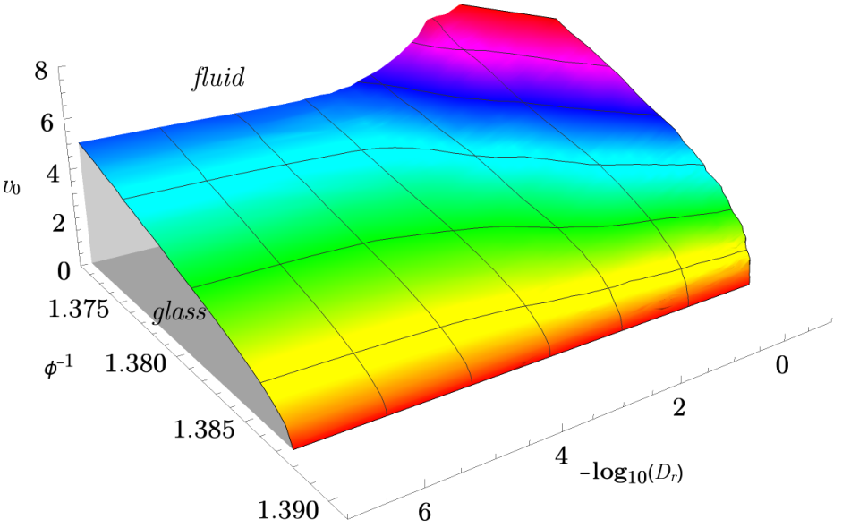
Figure 9 summarizes the estimated glass-transition points of the MCT transition of active hard disks as a critical surface in the parameter space spanned by $(1/\phi,\log_{10}(1/D_{r}),v_{0})$. This choice is motivated by a recent study of self-propelled cells in a self-propelled Voronoi fluid model by Bi et al. [5]. In this model, a self-adhesion parameter $p$ plays the role of an inverse density. In Ref. [5], an active-glass diagram was conjectured that includes two limiting shapes for $D_{r}\to 0$ and $D_{r}\to\infty$ with a cross-over between them around $D_{r}=1$. The numerical results shown in Fig. 9 are in good agreement with the conjecture by Bi et al. [5] over the range of $D_{r}$ shown. A glass-transition surface emerges that extends from a limiting line in the $(v_{0},1/\phi)$ plane at $D_{r}=0$ and bends upwards to higher $v_{0}$ as $D_{r}$ increases beyond $D_{r}\approx 0.01$. From the discussion above, one expects the glass-transition surface to bend over to a vertical plane as $D_{r}\to\infty$ (i.e., to the right of Fig. 9), different from what was suggested in Ref. [5].

Different from the case $D_{r}\to\infty$, the present MCT predicts a $v_{0}$-dependent limiting shape of the glass transition in the limit $D_{r}\to 0$. This glass transition is given by the bifurcation points of Eq. (25).

To characterize the glassy structure, we show in Fig. 10 the nonergodicity parameters of the positional-density correlation functions, $F_{00}(\vec{q})$, for different $v_{0}$ at fixed packing fraction. The passive case $v_{0}=0$ is included for reference; it shows the known features of $F_{00}(\vec{q})$: the nonergodicity paraeters oscillate in phase with the static structure factor. They are most pronounced around $q\sigma\approx 7$, indicating that the glass is stiffest with respect to density fluctuations of wavelengths comparable to the particle size.

Increasing $v_{0}$, the nonergodicity parameters decrease for all $q$. Thus, active driving renders the glass mechanically softer at fixed density. The effect is however minor: for most $q$, the values for $v_{0}=5\,D_{t}/\sigma$ are less than $10\%$ smaller compared to the passive case. The decrease in mechanical stiffness of the glass with increasing activity might be counter-intuitive: with increasing Péclet number $\mathit{Pe}$, the effective pressure of the system according to its low-density description increases [49]. Such an increase in pressure might, by analogy to the passive system, be expected to cause an increase in mechanical stiffness. This shows that active forces act quite differently from thermodynamic ones at the glass transition.

There is an interesting observation regarding the off-diagonal components of $\boldsymbol{F}(\vec{q})$: while $F_{l0}(\vec{q})=0$ for all $l\neq 0$, due to the presence of the hopping term $\propto l^{2}D_{r}$, the MCT equations admit solutions where $F_{0l}(\vec{q})\neq 0$ for all $l$. In particular $F_{01}(\vec{q})\neq 0$, as shown in Fig. 10. In other words, the active glass keeps infinite memory not only in the translational degrees of freedom, but also in the coupling of orientations to translations. Loosely speaking, an initial orientation fluctuation leaves its fingerprint in the positions in the glass, while of course an initial density fluctuation does not affect the later orientation fluctuations.

The non-trivial long-time limits $F_{01}(\vec{q})$ are shown in Fig. 11 for the same state points as those in Fig. 10. For the reference frame chosen in our discussion, the values of $F_{01}(\vec{q})$ are negative and real; note that this is not invariant under rotations of the coordinate system. Apart from this, the $F_{01}(\vec{q})$ show behavior that is qualitatively similar to the one seen in $F_{00}(\vec{q})$: oscillations are dictated by those in the equilibrium static structure factor, and the strongest conribution comes from nearest-neighbor cage distances.

The nonergodicity parameters discussed above are the values attained by the transient density correlation functions for large times, i.e., $D_{t}t/\sigma^{2}\gg 1$ and in particular $D_{r}t\gg 1$. In the case of strongly persistent motion, $D_{r}\ll D_{t}/\sigma^{2}$, an intermediate time window opens where $\sigma^{2}/D_{t}\ll t\ll 1/D_{r}$, i.e., for times large compared to the free diffusion time, but small compared to the timescale of reorientations.

References

- [1] M. Poujade, E. Grasland-Mongrain, A. Hertzog, J. Jouanneau, P. Chavrier, B. Ladoux, A. Buguin, and P. Silberzan, Proc. Natl. Acad. Sci. USA 104, 15988 (2007).
- [2] L. Petitjean, M. Reffay, E. Grasland-Mongrain, M. Poujade, B. Ladoux, A. Buguin, and P. Silberzan, Biophys. J. 98, 1790 (2010).
- [3] X. Trepat, M. R. Wasserman, T. E. Angelini, E. Millet, D. A. Weitz, J. P. Butler, and J. J. Fredberg, Nature Phys. 5, 426 (2009).
- [4] T. E. Angelini, E. Hannezo, X. Trepat, J. J. Fredberg, and D. A. Weitz, Phys. Rev. Lett. 104, 168104 (2010).
- [5] D. Bi, X. Yang, M. C. Marchetti, and M. L. Manning, Phys. Rev. X 6, 021011 (2016).
- [6] F. Peruani, J. Starruß, V. Jakovljevic, L. Søgaard-Andersen, A. Deutsch, and M. Bär, Phys. Rev. Lett. 108, 098102 (2012).
- [7] B. Fabry, G. N. Maksym, J. P. Butler, M. Glogauer, D. Navajas, and J. J. Fredberg, Phys. Rev. Lett. 87, 148102 (2001).
- [8] P. Bursac, G. Lenormand, B. Fabry, M. Oliver, D. A. Weitz, V. Viasnoff, J. P. Butler, and J. J. Fredberg, Nature Materials 4, 557 (2005).
- [9] S. Wang, T. Shen, and P. G. Wolynes, J. Chem. Phys. 134, 014510 (2011).
- [10] A. Erbe, M. Zientara, L. Baraban, C. Kreidler, and P. Leiderer, J. Phys.: Condens. Matter 20 (2008).
- [11] L. Baraban, M. Tasinkevych, M. N. Popescu, S. Sanchez, S. Dietrich, and O. G. Schmidt, Soft Matter 8, 48 (2012).
- [12] J. Palacci, C. Cottin-Bizonne, C. Ybert, and L. Bocquet, Phys. Rev. Lett. 105, 088304 (2010).
- [13] I. Buttinoni, J. Bialké, F. Kümmel, H. Löwen, C. Bechinger, and T. Speck, Phys. Rev. Lett. 110, 238301 (2013).
- [14] G. Volpe, I. Buttinoni, D. Vogt, H.-J. Kümmerer, and C. Bechinger, Soft Matter 7, 8810 (2011).
- [15] A. Zöttl and H. Stark, J. Phys.: Condens. Matter 28, 253001 (2016).
- [16] M. C. Marchetti, Y. Fily, S. Henkes, A. Patch, and D. Yllanes, Curr. Opin. Colloid Interf. Sci. 21, 34 (2016).
- [17] P. K. Ghosh, Y. Li, G. Marchegiani, and F. Marchesoni, J. Chem. Phys. 143, 211101 (2015).
- [18] R. Ni, M. A. C. Stuart, and M. Dijkstra, Nature Commun. 4, 2704 (2013).
- [19] Y. Fily, S. Henkes, and M. C. Marchetti, Soft Matter 10, 2132 (2013).
- [20] H.-S. Kuan, R. Blackwell, L. E. Hough, M. A. Glaser, and M. D. Betterton, Phys. Rev. E 92, 060501(R) (2015).
- [21] L. Berthier and J. Kurchan, Nature Phys. 9, 310 (2013).
- [22] L. Berthier, Phys. Rev. Lett. 112, 220602 (2014).
- [23] D. Levis and L. Berthier, EPL 111, 60006 (2015).
- [24] G. Szamel, E. Flenner, and L. Berthier, Phys. Rev. E 91, 062304 (2015).
- [25] R. Mandal, P. J. Bhuyan, M. Rao, and C. Dasgupta, Soft Matter 12, 6268 (2016).
- [26] S. C. Takatori, W. Yan, and J. F. Brady, Phys. Rev. Lett. 113, 028103 (2014).
- [27] S. C. Takatori and J. F. Brady, Curr. Opin. Colloid Interf. Sci. 21, 24 (2016).
- [28] W. Yan and J. F. Brady, Soft Matter 11, 6235 (2015a).
- [29] W. Yan and J. F. Brady, “The force on a boundary in active matter,” (2015b), cond-mat.soft/1510.07731 .
- [30] C. Kurzthaler, S. Leitmann, and T. Franosch, Sci. Rep. 6, 36702 (2016).
- [31] S. Wang and P. G. Wolynes, J. Chem. Phys. 135, 051101 (2011).
- [32] T. F. F. Farage and J. M. Brader, “Dynamics and rheology of active glasses,” (2014), cond-mat.soft/1403.0928 .
- [33] T. F. F. Farage, P. Krinninger, and J. M. Brader, Phys. Rev. E 91, 042310 (2015).
- [34] G. Szamel, Phys. Rev. E 93, 012603 (2015).
- [35] S. K. Nandi, “Activity is strength: More active systems are stronger glass formers,” (2016a), cond-mat.soft/1605.06073 .
- [36] S. K. Nandi, “Steady state of active systems is characterized by unique effective temperature,” (2016b), cond-mat.soft/1607.04478 .
- [37] W. Götze, Complex Dynamics of Glass-Forming Liquids (Oxford University Press, 2009).
- [38] M. Bayer, J. M. Brader, F. Ebert, M. Fuchs, E. Lange, G. Maret, R. Schilling, M. Sperl, and J. P. Wittmer, Phys. Rev. E 76, 011508 (2007).
- [39] H. Ding, M. Feng, H. Jiang, and Z. Hou, “Nonequilibrium glass transition in mixtures of active-passive particles,” (2015), cond-mat.soft/1506.02754 .
- [40] G. Szamel, Phys. Rev. E 90, 012111 (2014).
- [41] U. M. B. Marconi and C. Maggi, Soft Matter 11, 8768 (2015).
- [42] Z. Sadjadi, M. R. Shaebani, H. Rieger, and L. Santen, Phys. Rev. E 91, 062715 (2015).
- [43] D. Levis and L. Berthier, Phys. Rev. E 89, 062301 (2014).
- [44] E. Flenner, G. Szamel, and L. Berthier, “The nonequilibrium glassy dynamics of self-propelled particles,” (2016), cond-mat.soft/1606.00641 .
- [45] C. Reichhardt and C. J. Olson Reichhardt, Soft Matter 10, 7502 (2014).
- [46] T. Franosch, M. Fuchs, W. Götze, M. R. Mayr, and A. P. Singh, Phys. Rev. E 56, 5659 (1997).
- [47] S. Kämmerer, W. Kob, and R. Schilling, Phys. Rev. E 56, 5450 (1997).
- [48] R. Schilling, Phys. Rev. E 65, 051206 (2002).
- [49] J. Tailleur and M. E. Cates, Phys. Rev. Lett. 100, 218103 (2008).
- [50] M. Fuchs and M. E. Cates, Phys. Rev. Lett. 89, 248304 (2002).
- [51] I. Gazuz, A. M. Puertas, T. Voigtmann, and M. Fuchs, Phys. Rev. Lett. 102, 248302 (2009).
- [52] M. Enculescu and H. Stark, Phys. Rev. Lett. 107, 058301 (2011).
- [53] J. Tailleur and M. E. Cates, EPL 86, 60002 (2009).
- [54] J. Bialké, T. Speck, and H. Löwen, Phys. Rev. Lett. 108, 168301 (2012).
- [55] Jülich Supercomputing Centre, Journal of large-scale research facilities 2 (2016), 10.17815/jlsrf-2-121.