Globally Constructed Adaptive Local Basis Set for
Spectral Projectors of
Second Order Differential Operators
Abstract
Spectral projectors of second order differential operators play an important role in quantum physics and other scientific and engineering applications. In order to resolve local features and to obtain converged results, typically the number of degrees of freedom needed is much larger than the rank of the spectral projector. This leads to significant cost in terms of both computation and storage. In this paper, we develop a method to construct a basis set that is adaptive to the given differential operator. The basis set is systematically improvable, and the local features of the projector is built into the basis set. As a result the required number of degrees of freedom is only a small constant times the rank of the projector. The construction of the basis set uses a randomized procedure, and only requires applying the differential operator to a small number of vectors on the global domain, while each basis function itself is supported on strictly local domains and is discontinuous across the global domain. The spectral projector on the global domain is systematically approximated from such a basis set using the discontinuous Galerkin (DG) method. The global construction procedure is very flexible, and allows a local basis set to be consistently constructed even if the operator contains a nonlocal potential term. We verify the effectiveness of the globally constructed adaptive local basis set using one-, two- and three-dimensional linear problems with local potentials, as well as a one dimensional nonlinear problem with nonlocal potentials resembling the Hartree-Fock problem in quantum physics.
keywords
Adaptive local basis; Discontinuous Galerkin; Spectral projector; Differential operator; Global construction; Random sampling; Quantum physics1 Introduction
Consider the second order differential operator
| (1) |
where is a rectangular, bounded domain in with periodic boundary conditions. is a real, bounded and smooth potential function. Then is a self-adjoint operator on . Using the eigen-decomposition , a spectral projector is an integral operator with its kernel defined as
| (2) |
Here is an interval that can be interpreted as an energy window indicating the eigenfunctions of interest, is an indicator function, and is the complex conjugation of . Denote by the number of eigenfunctions in the summation of Eq. (2), then the rank of is . We assume that is large, which can range from hundreds to hundreds of thousands. The spectral projector of such a form or of similar forms arises in many scientific and engineering problems. One notable example is the widely used Kohn-Sham density functional theory [20, 23] in quantum physics, where contains the lowest eigenvalues of . Typically, a large number of degrees of freedom associated with a fine numerical discretization are required to resolve the local features of ’s with sufficient accuracy. This is the case when standard discretization methods such as finite difference, finite element, discontinuous Galerkin, planewave, and wavelet type of methods are used. The ratio between the total number of degrees of freedom (DOFs) and can range from hundreds to hundreds of thousands in quantum physics applications [2, 40, 13]. As a consequence, both the storage cost and the computation cost associated with the spectral projector can be large.
1.1 Contribution
In this paper, instead of using a general basis set, we introduce a new basis set that can be specifically tailored to represent the spectral projector , for a given operator and an interval . The key observation is as follows. Let us partition into a suitable collection of non-overlapping sub-domains called elements. If the size of each element is small enough, then the numerical rank (a.k.a. the approximate rank up to certain truncation tolerance [16]) of each row block of restricted to any element can be bounded by a small constant. We shall quantify the details of the statement above later in the paper. The singular value decomposition of one such row block of defines the optimal basis set on an element. Since the local features of the range of is directly built into the basis set, we can expect that the number of degrees of freedom in such an optimal basis set is much smaller than that in a general basis set. However, such an optimal basis set cannot be practically obtained, since it requires the knowledge of a priori. We devise a numerical algorithm to compute a nearly optimal basis set. This is done by applying an approximate spectral projector, characterized by a matrix function , to a small number of random vectors defined on the global domain . The number of random vectors is only slightly larger than the approximate rank of restricted to each element. The range of is then approximately a subspace of the span of this basis set, and we find that this is an efficient and accurate way to generate the basis functions on all elements. Due to the non-overlapping condition, each basis function is only supported on one element, and is discontinuous on the global domain . We use the discontinuous Galerkin (DG) method [4] to patch the basis set to obtain an approximation to or . Motivated by our previous work of the locally constructed adaptive local basis set (LC-ALB) [29, 49, 21], the basis set in this work is dubbed the globally constructed adaptive local basis set (GC-ALB). The LC-ALB approach has already been demonstrated to be able to be executed efficiently on massively parallel computers with over processes, and to efficiently perform large scale Kohn-Sham density functional theory calculations for systems over atoms [21, 7].
The GC-ALB set has the following advantages: 1) Systematically improvable. As the number of basis functions in each element increases, the accuracy of the projector represented in this basis set systematically improves towards the converged spectral projector. 2) Efficient. The number of basis functions is directly related to the numerical rank of the row blocks of the projector, and is much smaller compared to the number of degrees of freedom needed to resolve the local shape of in the real space. The strict locality of the basis set can significantly reduce the computation and storage cost for and . 3) Flexible. The construction of the basis set only requires matrix-vector multiplication of defined on the global domain . This allows existing matrix-vector multiplication routines for computing to be readily used without the need of constructing auxiliary operators. This also facilitates generalizations to operators beyond the form in (1). This can occur e.g. for , where is an integral operator and hence becomes a nonlocal operator. Such an operator arises in applications such as the Kohn-Sham density functional theory with hybrid exchange-correlation functionals [8, 19] and the Hartree-Fock theory in quantum physics.
1.2 Related work
In the context of quantum physics, many tailored basis set have been designed to reduce the number of DOFs to represent spectral projectors (or density matrices in physics terminology). Notable examples include the Gaussian basis set and the atomic orbital basis set [45, 38, 10]. Such basis sets are developed based on physical intuition, and can provide relatively accurate solution with much reduced number of degrees of freedom compared to more conventional basis sets. However, expert knowledge is often required to systematically converge the solution. These basis sets have also been used to “enrich” conventional basis sets to achieve a balance between the small number of DOFs and the systematic convergence property [43, 46]. However, the number of DOFs in the mixed basis representation is often much larger than those using Gaussian orbital or atomic orbital basis sets alone.
In order to achieve systematic convergence without sacrificing the number of DOFs, one may give up the concept of designing a basis set a priori, but instead generate the basis set on the fly. This has been demonstrated via a number of approaches based on filtration [29, 33, 41, 12, 37] as well as optimization [44, 30, 11, 36] principles. A common ingredient of these methods is to truncate the operator into a series of operators defined only on different sub-domains, and the basis set is then generated from the truncated operators. This requires each basis function to satisfy zero Dirichlet boundary conditions at each subdomain, which is not always achievable without sacrificing the accuracy of the resulting basis set. The method in this paper only uses matrix-vector multiplication on the global domain, and hence the concern from the choice of boundary conditions on local domains is completely removed. Our numerical results indicate that the GC-ALB set can also be more efficient than the LC-ALB set measured in terms of the number of DOFs to reach the same target accuracy. The partition of unity method (PUM) [6] is another commonly used option for enriching the basis set using local basis functions. Compared to PUM, the basis functions in the DG approach are strictly localized in non-overlapping elements, and hence are often better conditioned. In fact, one can easily obtain an orthonormal basis set in the DG approach through a local orthonormalization procedure. This also facilitates the usage of efficient numerical techniques such as the Chebyshev filtering techniques [51] for the computation of spectral projectors.
1.3 Outline of the paper
The rest of the paper is organized as follows. We review the interior penalty formulation of the discontinuous Galerkin framework, introduce the optimal discontinuous basis set and the locally constructed adaptive local basis set in section 2. We present the globally constructed adaptive local basis set in section 3. The numerical results are given in section 4, followed by the conclusion and discussion in section 5.
2 Preliminaries
2.1 Discontinuous Galerkin method
Without loss of generality, let where , and be a regular partition of into a set of non-overlapping elements. For , we denote by the closure of . For any two elements , The periodic boundary condition on implies that the partition is regular across the boundary . We remark that generalizations to other boundary conditions such as Dirichlet or Neumann boundary conditions, as well as to non-rectangular domains, can be done with minor modification.
We denote by the standard Sobolev space of -functions such that the first partial derivatives are also in . We denote the set of piecewise -functions by
which is also referred to as the broken Sobolev space. For , the inner product is
| (3) |
which induces a norm .
For and , define the jump and average operators on a face by
| (4) |
and
| (5) |
where denotes the exterior unit normal of the element .
In order to numerically solve the eigenvalue problem
we need to identify a basis set which spans a subspace of . Let be the number of DOFs on , and the total number of DOFs is . Let , where each is a function defined on with compact support only in . Hence is a subspace of and is associated with a finite dimensional approximation for . Then is a finite dimensional approximation to . We also assume all functions form an orthonormal set of vectors in the sense that
| (6) |
The interior penalty formulation of the discontinuous Galerkin method [4] introduces the following bilinear form
| (7) |
Here the terms in the first bracket corresponds to the operator . The terms in the second bracket are obtained from integration by parts, and the terms in the third bracket is a penalty term to guarantee the stability of the bilinear form [5]. The penalty parameter on each element needs to be large enough, and the value of depends on the choice of basis set . For general non-polynomial basis functions the value of is not known a priori. One possible solution is given in [31] which provides a formula for evaluating on the fly for general non-polynomial basis sets based on the solution of eigenvalue problems restricted to each element .
Using the bilinear form (7), the solution of
| (8) |
gives the numerical solution of eigenpairs of the form and . Eq. (8) can be equivalently written as a standard linear eigenvalue problem
| (9) |
where satisfies , and the reduced matrix is of size with matrix elements
| (10) |
Using the solution of Eq. (9), we can select and obtain an approximation to the spectral projector
| (11) |
Here is the matrix representation of in the basis set , and
| (12) |
2.2 Optimal discontinuous basis set
The discontinuous Galerkin method in section 2.1 can be applied to very general basis sets . Here we consider the optimal basis set for representing the spectral projector with a discontinuous basis set. To simplify the discussion below, we also use linear algebra notation in this section when necessary. This means that we may not distinguish the kernel of an operator and a finite dimensional matrix consisting of its nodal values discretized on a fine set of real space grid points, with the number of grid points denoted by . Then notation such as can be real space grid points in , or row / column indices of vectors / matrices. We call a row vector, and a column vector, respectively. Similarly, we call a row block, and a column block, respectively.
Since the rank of the spectral projector is , if we choose a partition fine enough we may expect that the numerical rank of each row block becomes small. In particular, note that the rank of cannot exceed the number of degrees of freedom in , which is a constant and is independent of . Our numerical results indicate that this rank can often be much lower than the number of degrees of freedom in in practice. The singular value decomposition (SVD) of can be written as
| (13) |
where is a diagonal matrix containing the leading singular values on , and for . The support of each function is strictly in . Since ’s are generated from the SVD of , clearly the range of is approximately contained in . For a given , the basis achieves the smallest error in 2-norm for representing thanks to the optimal approximation property of the SVD [16] using basis functions. Hence the basis set can be regarded as the optimal discontinuous basis set for representing for a given set of degrees of freedom . We illustrate the decomposition (13) for the entire spectral projector in Fig. 1.

2.3 Locally constructed adaptive local basis set
The optimal discontinuous basis set cannot be used for practical computation, since its construction depends on the knowledge of . One possible approximation of such a basis set using non-polynomial basis functions is the adaptive local basis (ALB) set [29]. More specifically, we refer to this basis set the locally constructed adaptive local basis (LC-ALB) set, in order to distinguish from the globally constructed adaptive local basis set in section 3.
Consider the case that contains the lowest eigenvalues of . In the -dimensional space, for each element , we form an extended element around , and we refer to as the buffer region for . Fig. 2 illustrates a particular together with its butter region. On we solve the eigenvalue problem
| (14) |
with certain boundary conditions on . This eigenvalue problem can be solved using standard basis set such as finite difference, finite elements, or planewaves. For the numerical examples in this paper, the periodic boundary conditions is applied on each , and the eigenvalue problem is solved via the pseudo-spectral method (the planewave basis set). Note that the size of the extended element is independent of the size of the global domain, and so is the number of basis functions per element. In order to obtain , the eigenfunctions corresponding to lowest eigenvalues are restricted from to , i.e.
After orthonormalizing locally on each element and removing the linearly dependent functions via a local singular value decomposition, the resulting set of orthonormal functions form the LC-ALB set.

The advantage of the LC-ALB set is that the basis functions for each element can be generated completely independently. However, due to the fictitious boundary conditions imposed on the extended element , the effectiveness of the LC-ALB set depends on the size of the buffer region. On one extreme, if the size of the buffer region is and when the periodic boundary condition is used, since is in general not a periodic function on , the accuracy of the basis set can be severely affected by the Gibbs phenomena. On the other hand, if the buffer region is chosen to be too large, then the solution of the local eigenvalue problem (14) can become expensive. In practice we find that choosing to contain and its neighboring elements yields a relatively good balance between efficiency and accuracy, as has been demonstrated by the usage for solving PDEs [31, 32] and for solving practical Kohn-Sham equations [29, 21].
3 Globally constructed adaptive local basis set
In this section, we propose a new strategy to construct an approximation to the optimal discontinuous basis set by using matrix-vector multiplication involving the operator defined on the global domain . This allows us to overcome the difficulty of choosing the boundary condition and the size of the extended element as in the LC-ALB set. Numerical results indicate that the resulting basis set is more effective in terms of the number of DOFs, and the strategy can be adapted to more general cases such as when is an integral operator with a nonlocal kernel.
3.1 Formulation
We first introduce Algorithm 1, which is a variant of e.g. Algorithm 4.1 in [18] for finding the approximate range of a numerically low rank matrix.
If we treat as a dense matrix and apply the SVD directly, the computational complexity will be . On the other hand, Alg. 1 only requires applying the matrix to vectors, together with the SVD for which costs operations. Hence the randomized range finder algorithm significantly reduces the cost, if is much smaller than and if the matrix vector multiplication can be evaluated quickly. Usually, step 2 is the most expensive operation in Algorithm 1.
Assume is a partition of so that each matrix row block is a numerically low rank matrix. If we apply Algorithm 1 to , the output gives highly accurate approximation to the optimal basis set for . Furthermore, the random matrix can be repeatedly used for different . Therefore, the matrix-vector multiplication for different matrix row blocks do not need to be applied independently. Instead it is equivalent to apply the entire matrix to a random matrix , and to perform the SVD for each element independently to obtain an approximate range represented by for each . The collection of the functions gives the globally constructed adaptive local basis set (GC-ALB). Algorithm 2 describes this procedure for a general matrix , where is the number of DOFs corresponding to a fine numerical discretization such as planewaves.

When taking the matrix to be the spectral projector , Fig. 3 illustrates Alg. 2 for the case that is partitions the domain into elements. Comparing to Fig. 1 where each block of is explicitly factorized, Fig. 3 first applies to random vectors and then factorizes each block of . Such an extra step is crucial here. Computing the dense is expensive in terms of both computation and memory, whereas the matrix vector multiplication can be efficiently calculated, which could be orders of magnitudes faster for large problems.
3.2 Rational approximation for matrix-vector multiplication
In order to construct the GC-ALB set for the projector , Alg. 2 requires an efficient method to compute the matrix-vector multiplication . Since the spectral projector is a non-smooth matrix function , the computation of may still be a costly procedure. Fortunately, we only need Alg. 2 to find an approximate range of . Hence we may replace by a smooth function , with the requirement that the support of covers the interval , and that is relatively easy to compute. Then we can apply Alg. 2 to find the approximate range of . The choice of is certainly not unique. Here we use a modified Zolotarev’s function to be , which is an optimal rational approximation to the indicator function as to be demonstrated below.
Without loss of generality, we assume that in the following discussion. Zolotarev’s function was initially proposed as the best rational approximant of type for the signum function on the interval with a positive parameter [52, 1]. Recently, it was composed with a Möbius transformation and a linear transformation [17, 25] to become the best rational approximant of type for an indicator function on the interval , where and are two parameters such that and . Both the Möbius transformation and the parameter in Zolotarev’s function depend on and . To be more precise, the Möbius transformation is defined as follows,
| (15) |
with and such that
| (16) |
Here, the variables and are determined by and via solving the equations in (16). Combining with a simple linear transformation, , we arrive at a modified Zolotarev’s function,
| (17) |
where is the same as in (15), and are constants as defined in [25], and denotes the complex conjugate. are known as the poles of the modified Zolotarev’s function.
When the modified Zolotarev’s function is used as , and the matrix in Alg. 2 is replaced by , the line in Alg. 2 can be evaluated via,
| (18) |
This requires solving complex-shifted linear systems, where denotes the identity matrix of the same size as . If both and are real matrices, then is the complex conjugate of . Therefore, solving shifted linear systems in (18) can be reduced to solving shifted linear systems instead. These shifted linear systems can be solved via standard iterative methods such as GMRES [42] and MINRES [39] with a preconditioner. The condition number of the shifted linear systems depends on the minimal distance between the eigenvalues of and the shifts , as well as the spectral radius of . The minimal distance can be systematically controlled by tuning the smoothness of the function , through the adjustment of the interval and . When the spectral radius of is large such as in the case of the planewave discretization, we find that the inverse of a shifted Laplacian [48] is an efficient preconditioner to reduce the condition number. Therefore, as shown in the numerical results, the number of iterations needed for solving the linear systems can be systematically controlled and relatively small.


Through the discussion above, the choice of and remains to be determined. For a fixed indicator function with the given interval , and determine the quality of the approximation of the modified Zolotarev’s function in (17). Generally, if either interval or becomes too narrow, it may require a large number of terms in (18) to reach the same target accuracy. This translates to solving more shifted linear systems. However, the situation simplifies when covers the lowest eigenvalues of , as will be demonstrated in the numerical results. Let the eigenvalues of be . The parameter can be an arbitrary number in , and we can set to be . The choice of relies on the spectrum property of around . When there is an eigenvalue gap around , i.e., , is set to be or its estimated lower bound calculated via a few steps of Lanczos method [51]. In the case that has continuous spectrum around , we construct a small gap as and for some small positive constant . The consequence of such a gap is that the approximated projector of would include extra eigenvectors with non-zero weights. In practice, we find that the GC-ALB method is robust to this choice of . Such an observation even allows us to choose to be larger than even in the presence of a gap, in order to reduce and hence the computational cost. When the location of is not known a priori, similar to the situation in Chebyshev filtering techniques [51, 50], the initial guess of can be efficiently obtained through a few Lanczos [24] iterations in practice.
Fig. 4 gives an example of the modified Zolotarev’s function for the approximation of where . We assume is in the continuous spectrum of . We choose and so that is sufficient to approximate the indicator function with error below in the interval .
3.3 Complexity
In practical computation of the spectral projector, the following two scenarios are often encountered when counting the complexity with respect to the increase of the number of DOFs.
- 1.
The size of the global domain is fixed, and the number of DOFs increases due to the refinement of the discretization.
- 2.
The size of the global domain increases, and the number of DOFs increases proportionally to the volume of .
Let be the number of elements in , and be the number of DOFs corresponding to a fine discretization on the global domain. For simplicity let all elements have the same number of basis functions denoted by , and the number of DOFs corresponding to a fine discretization on is . Hence the total number of basis functions is . We also assume is bounded by a constant while can increase. In scenario 1, we increase and fix . In scenario 2, is proportional to while the ratio is fixed.
The computational cost of the matrix vector multiplication associated with applying to random vectors is . Here is the number of poles in the rational approximation, is the number of iterations to solve for each pole, and is the cost of per iteration. Since is a smooth function, is bounded by a constant independent of . When a good preconditioner is available, can also be bounded by a constant. often is dominated by the matrix-vector multiplication associated with . Furthermore, when is a local potential and when the planewave basis set is used, the cost of applying is dominated by applying the Laplacian operator which can be performed using the fast Fourier transform (FFT). Then . Since is fixed, in both scenarios the cost of the matrix-vector multiplication is . The cost of each SVD in step 4 is , and the cost for all SVDs is . Hence the overall complexity for constructing the GC-ALB set is . Note that the LC-ALB approach uses a domain decomposition method, and the computational complexity of is trivially . However, GC-ALB removes redundant calculations due to overlapping extended elements, and our numerical results indicate that the efficiency of the GC-ALB approach can be comparable or even faster when compared to LC-ALB.
The use of the GC-ALB set can also significantly reduce the storage cost for the spectral projector . The storage cost for the GC-ALB set is . Viewed as a matrix, the storage cost for is . This is generally very expensive, and is usually stored using a low rank format as , where is of size . Then the storage cost for the coefficient matrix as in Eq. (9) is , and the total storage cost for representing in the GC-ALB set is . Hence when the rank of the projector satisfies
the use of the GC-ALB set leads to reduction in the storage cost for . In practical applications such as Kohn-Sham equations, this condition is easy to satisfy since increases with respect to the system size, while is usually a constant on the order of .
Similarly, the computational cost for using standard iterative eigensolvers is asymptotically dominated by the need of orthonormalizing when is large. The complexity of this orthonormalization step scales as . In the GC-ALB set is constructed, the cost for the orthonormalization is reduced to .
Alg. 2 for constructing the GC-ALB set can also be efficiently parallelized. For the computation of , which is often the most time consuming step, the solution of the shifted linear systems for each column of are all independent of each other. Therefore, the computation can be embarrassingly parallelized up to processors. If more than processors are available, they will be organized into processor groups, and the application of can be parallelized as well. For the second part of Alg. 2, all calculations can be carried out independently on each element.
3.4 Generalization to nonlocal potentials
Another advantage of the GC-ALB approach is that it handles local and nonlocal potentials on the same footing. The need of computing spectral projectors associated with nonlocal potentials arise, for instance, in solving the Hartree-Fock-like equations in quantum chemistry [47, 34]. The Hartree-Fock-like equations require the self-consistent computation of the projector
| (19) |
Here the interval contains the lowest eigenvalues of . are local potentials, and is an integral operator with a nonlocal kernel. Here indicates the nonlinear dependence with respect to . There is no natural way to consistently incorporate the nonlocal term in the LC-ALB approach, while GC-ALB only requires the matrix-vector multiplication associated with . A detailed example of Eq. (19) will be given in section 4.2.
4 Numerical examples
We demonstrate the effectiveness of the GC-ALB method for finding the spectral projector for a linear problem in one, two and three dimensions in section 4.1, and for a nonlinear problem in one dimension in section 4.2. Numerical examples are performed on Stanford Sherlock cluster bigmem node with quad socket Intel(R) Xeon(R) CPU E5-4640 @ 2.40GHz and 1.5 TB RAM. In all numerical examples, we assume the global domain satisfies the periodic boundary condition. The pseudo-spectral discretization (a.k.a. the planewave basis set) provides the reference solution to the spectral projector, as well as the discretized operator for performing the matrix-vector multiplication on the global domain in order to construct the GC-ALB set. We measure the accuracy of the DG based methods in terms of the relative error of the eigenvalues within the range of the spectral projector compared to the reference solution, defined as
The pseudo-spectral discretization can be identified with a set of uniform grid to discretize . The integrals needed to construct the DG bilinear form is done using the Legendre-Gauss-Lobatto (LGL) grid. A Fourier interpolation procedure is used to interpolate functions from the uniform grid to the LGL grid, and a stable barycentric Lagrange interpolation [9] procedure is used to interpolate functions from the LGL grid back to the uniform grid when needed. In the rational approximation for the matrix vector multiplication, 16 poles on the upper half complex plain are actually solved. Since the potential function in all numerical examples are real, the rest of the 16 poles are evaluated via the complex conjugation as in Eq. (18). For each pole, we use the GMRES [42] method to solve the associated equations with 30 being the restarting number and being the tolerance. The preconditioner is the inverse of a shifted Laplacian [48] with the pole being the shift, which can be carried out efficiently using fast Fourier transforms (FFT). The oversampling parameter in Alg. 2 is set to be 5. All pseudo-spectral discretized systems, including the systems for the reference solutions and the system on each extended element in LC-ALB method, are solved via the LOBPCG [22] method, and the associated tolerance is measured in terms of the maximal residual norm. We use the interior penalty formulation to patch the discontinuous basis functions to approximate the eigenfunctions, and the penalty parameter is determined automatically by solving a local eigenvalue problem as in [31].
4.1 Linear problems with local potentials
4.1.1 One dimensional case
Our first example is a second order differential operator (1) on in 1D. is a local potential with four Gaussian potential wells at positions . The depth for each well is whereas the standard deviation is set to be . Fig. 5 (a) shows the potential . The interval associated with the spectral projector is assumed to cover the lowest 16 eigenvalues.
The global domain is partitioned into elements. Within each element, LGL grid points are used to evaluate the integrals in the DG bilinear form accurately. The pseudo-spectral method discretizes using planewave basis functions, which can be identified with a uniform grid with grid points. Under these settings, three adaptive local basis construction methods are considered, i.e., LC-ALB, GC-ALB with rational approximation for the projector (GC-ALB), and the optimal basis set (Opt). For different methods, we vary the number of basis functions used in each element from 6 to 14. The relative error of the smallest 16 eigenvalues is measured against a reference solution, which is calculated via the pseudo-spectral method with 500 planewave basis functions directly. In the GC-ALB, we set the interval as and the gap parameters as and , where and denote the smallest eigenvalue and the 16th smallest eigenvalue, respectively. Fig. 5 (b) shows the relative errors for different methods with varying number of basis functions. More details are reported in Tab. 1.


| Method | err | (sec) | (sec) | ||
|---|---|---|---|---|---|
| GC-ALB | 6 | 1.41e-04 | 5.69e-01 | 1.12e-02 | 147 |
| 8 | 2.27e-08 | 6.14e-01 | 1.06e-02 | 147 | |
| 10 | 1.65e-11 | 6.22e-01 | 1.18e-02 | 148 | |
| 12 | 7.64e-14 | 7.21e-01 | 1.49e-02 | 149 | |
| 14 | 2.41e-14 | 7.24e-01 | 1.26e-02 | 150 | |
| LC-ALB | 6 | 4.45e-04 | 2.91e-01 | 1.05e-02 | - |
| 8 | 4.93e-06 | 3.24e-01 | 1.06e-02 | - | |
| 10 | 2.51e-09 | 3.59e-01 | 1.55e-02 | - | |
| 12 | 3.71e-11 | 3.91e-01 | 1.42e-02 | - | |
| 14 | 1.93e-13 | 4.20e-01 | 1.25e-02 | - |
For the one dimensional operator, as shown in Fig. 5 (b), the relative errors for all three methods decay exponentially as the number of basis functions increases. As discussed in section 2.2, the Opt basis defines the optimal discontinuous basis set for a given partition of the global domain and number of basis functions in each element, and this is confirmed in Fig. 5 (b). On the other hand, the performance both GC-ALB and LC-ALB closely follow the Opt basis. Given the same number of basis functions, GC-ALB is about one digit more accurate than LC-ALB. When the number of basis functions is larger than or equal to 14, both methods reach the numerical accuracy limit and can not be further improved. The runtime of the GC-ALB method and LC-ALB are about the same. The numbers of total iterations are about 148, which means the iteration number for solving each pole in (18) is on average smaller than 10.
4.1.2 Two dimensional case
This example is a second order differential operator (1) on in 2D. is a local potential with four Gaussian wells as shown in Fig. 6 (a). The depth for each well is and the standard deviation is . Similar to one dimensional example, the interval associated with the spectral projector is assumed to cover the lowest 16 eigenvalues.
The global domain is partitioned into elements. Within each element, two dimensional LGL grid points are used to evaluate the integrals in the DG bilinear form accurately. The pseudo-spectral method discretizes using planewave basis functions, which can be identified with a uniform two dimensional grid with grid points. Similar name conventions for LC-ALB, GC-ALB and Opt are used as in the one dimensional example. For different methods, we vary the number of basis functions used in each element from 8 to 22. The relative error of the smallest 16 eigenvalues is measured against a reference solution, which is calculated via the pseudo-spectral method with planewave basis functions directly. In the GC-ALB, we set the interval as and the gap parameters as and , where and denote the smallest eigenvalue and the 16th smallest eigenvalue. Fig. 6 (b) shows the relative errors for different methods with varying number of basis functions. More details are reported in Tab. 2.


| Method | err | (sec) | (sec) | ||
|---|---|---|---|---|---|
| GC-ALB | 6 | 5.27e-02 | 2.72e+01 | 2.53e-01 | 156 |
| 8 | 1.13e-02 | 2.95e+01 | 2.80e-01 | 156 | |
| 10 | 2.43e-03 | 3.37e+01 | 3.29e-01 | 156 | |
| 12 | 6.67e-04 | 3.71e+01 | 3.95e-01 | 156 | |
| 14 | 5.98e-05 | 3.83e+01 | 4.76e-01 | 156 | |
| 16 | 9.99e-06 | 4.15e+01 | 4.61e-01 | 156 | |
| 18 | 2.98e-06 | 4.12e+01 | 6.31e-01 | 156 | |
| 20 | 4.10e-08 | 4.59e+01 | 6.51e-01 | 157 | |
| 22 | 6.87e-14 | 4.99e+01 | 6.78e-01 | 156 | |
| LC-ALB | 6 | 2.27e-01 | 1.41e+01 | 2.21e-01 | - |
| 8 | 2.25e-02 | 1.49e+01 | 2.45e-01 | - | |
| 10 | 5.53e-03 | 2.59e+01 | 3.12e-01 | - | |
| 12 | 2.75e-03 | 2.52e+01 | 3.75e-01 | - | |
| 14 | 1.67e-03 | 3.30e+01 | 4.75e-01 | - | |
| 16 | 6.95e-04 | 2.76e+01 | 5.17e-01 | - | |
| 18 | 2.69e-04 | 2.85e+01 | 5.90e-01 | - | |
| 20 | 1.05e-04 | 2.90e+01 | 6.21e-01 | - | |
| 22 | 6.37e-05 | 4.38e+01 | 7.39e-01 | - |
Fig. 6 (b) shows that the differences among LC-ALB, GC-ALB and Opt basis sets become more significant in 2D. The relative errors for Opt and GC-ALB decreases to the level of when 16 and 22 basis functions are constructed for each element respectively. On the other hand side, the relative errors for LC-ALB method remains around when basis functions are used for each element. In order to achieve an relative error that is below , we also find that basis functions per element are needed in the LC-ALB approach. Tab. 2 shows that the cost for the GC-ALB and LC-ALB approaches are comparable in 2D. The fluctuation of the runtime in the LC-ALB approach is mostly due to the fluctuation of the number of iterations for the LOBPCG solver. In the GC-ALB approach, the number of iterations for solving each pole here is around 9 on average for all cases, which gives to be around in all cases.
Below we demonstrate the weak scaling performance of the GC-ALB set in 2D. Starting from the potential in Fig. 6 (a), we increase the size of the domain by periodically repeating the potential along and directions by a factor of . We vary from 1 to 6, as shown in Tab. 3, and the domain is extended from to . The number of planewave basis functions, the number of elements, as well as the number of eigenvalues to be computed are proportional to the size of . The parameters used within each element are the same as before and 20 basis functions are constructed for each element. In terms of the parameters in Zolotarev’s function approximation, we set the interval as and the gap parameters as and , where and denote the smallest eigenvalue and the th smallest eigenvalue. The relative error of the smallest eigenvalues is measured against reference solutions, which are calculated via the pseudo-spectral method with planewave basis functions directly. Since the reference solution for cannot be finished within the limited runtime on the Sherlock system, only the GC-ALB runtime and the total iteration number are reported here.
| err | (sec) | (sec) | ||||
|---|---|---|---|---|---|---|
| 1 | 16 | 1.14e-07 | 4.97e+01 | 8.74e-01 | 156 | |
| 2 | 64 | 4.47e-07 | 3.17e+02 | 6.29e+00 | 197 | |
| 3 | 144 | 5.78e-07 | 6.21e+02 | 4.64e+01 | 209 | |
| 4 | 256 | 7.29e-07 | 2.09e+03 | 1.87e+02 | 271 | |
| 5 | 400 | 6.33e-07 | 3.53e+03 | 6.11e+02 | 268 | |
| 6 | 576 | - | 7.52e+03 | 1.66e+03 | 268 |


Tab. 3 shows that the relative errors are approximately the same for all . The runtime, , for the basis construction in GC-ALB increases proportional to , which means is quasi-linear in the number of planewave basis functions (see Fig. 7 (a)). Meanwhile , which is the cost for solving the DG problem is super-linear with respect to the number of planewave basis functions (see Fig. 7 (b)). is consist with the complexity analysis and is close aligned with the complexity analysis when is large. We observe that when is relatively small, the number of total iterations mildly increases with respect to . As keeps on increasing, the total iteration number stays around .
4.1.3 Three dimensional case
This example is a second order differential operator (1) on in 3D. is a local potential with four Gaussian wells. The depth for each well is whereas the standard deviation is set to be . Fig. 6 (a) shows the isosurface for the potential function . Similar to previous examples, the interval associated with the spectral projector is assumed to cover the lowest 16 eigenvalues.
The global domain is partitioned into elements. Within each element, three dimensional LGL grid points are used to evaluate the integrals in the DG bilinear form accurately. The pseudo-spectral method discretizes using planewave basis functions, which can be identified with a uniform three dimensional grid with grid points. Similar name conventions for LC-ALB, GC-ALB and Opt are used as in the one dimensional example. For different methods, we vary the number of basis functions used in each element from 8 to 24. The relative error of the smallest 16 eigenvalues is measured against a reference solution, which is calculated via the pseudo-spectral method with planewave basis functions directly. In the GC-ALB, we set the interval as and the gap parameters as and , where and denote the smallest eigenvalue and the 16th smallest eigenvalue. Fig. 8 (b) shows the relative errors for different methods with varying number of basis functions. More details are reported in Tab. 4.


| Method | err | (sec) | (sec) | ||
|---|---|---|---|---|---|
| GC-ALB | 6 | 9.89e-01 | 1.52e+02 | 3.07e+00 | 128 |
| 8 | 5.15e-01 | 1.60e+02 | 3.60e+00 | 128 | |
| 10 | 1.01e-01 | 2.07e+02 | 4.34e+00 | 129 | |
| 12 | 4.24e-02 | 1.81e+02 | 4.87e+00 | 129 | |
| 14 | 1.64e-02 | 2.43e+02 | 5.68e+00 | 129 | |
| 16 | 5.76e-03 | 2.40e+02 | 6.48e+00 | 129 | |
| 18 | 9.42e-04 | 2.89e+02 | 7.66e+00 | 129 | |
| 20 | 2.92e-11 | 3.04e+02 | 8.30e+00 | 129 | |
| 22 | 9.63e-12 | 3.19e+02 | 8.84e+00 | 129 | |
| 24 | 1.65e-11 | 3.51e+02 | 1.23e+01 | 129 | |
| LC-ALB | 6 | 1.62e+00 | 5.25e+02 | 3.15e+00 | - |
| 8 | 8.84e-01 | 2.02e+03 | 3.31e+00 | - | |
| 10 | 7.32e-01 | 1.54e+03 | 5.23e+00 | - | |
| 12 | 5.73e-01 | 1.22e+03 | 6.18e+00 | - | |
| 14 | 3.04e-01 | 1.16e+03 | 7.05e+00 | - | |
| 16 | 6.48e-02 | 1.26e+03 | 7.82e+00 | - | |
| 18 | 1.79e-02 | 1.46e+03 | 9.00e+00 | - | |
| 20 | 5.00e-03 | 1.87e+03 | 9.19e+00 | - | |
| 22 | 5.02e-03 | 1.81e+03 | 1.07e+01 | - | |
| 24 | 5.04e-03 | 1.96e+03 | 1.20e+01 | - |
| err | DOFs | err | DOFs | ||||
|---|---|---|---|---|---|---|---|
| GC-ALB | 14 | 1.69e-02 | 896 | planewave | 16 | 9.50e-03 | 4096 |
| 16 | 4.34e-03 | 1024 | 20 | 2.13e-03 | 8000 | ||
| 18 | 1.36e-04 | 1152 | 26 | 1.60e-04 | 17576 | ||
| 20 | 9.19e-12 | 1280 | 60 | 1.10e-10 | 216000 |
For three dimensional systems, the GC-ALB method exhibits even clearer advantage over the LC-ALB method. In Fig. 8 (b) and Tab 4, the relative errors for GC-ALB method decay quickly to the level of , while the asymptotic decay rate of the LC-ALB method is much slower. The GC-ALB approach is also more efficient in terms of the runtime. For most of the cases in Tab 4, the GC-ALB method is about 6 times faster than LC-ALB method. The numbers of the applications of the operator to test vectors are 129 in GC-ALB method for all different number of bases. In addition, Tab. 5 shows that the number of DOFs for the GC-ALB set is much smaller than that needed for the planewave basis set to reach the same level of accuracy. Here the DOFs for the GC-ALB set is equal to the dimension of the DG matrix, and the DOFs for the planewave basis set is the number of planewave basis functions.
4.2 Nonlinear problems with nonlocal potentials
In order to test the effectiveness of the GC-ALB approach for nonlocal potentials, we consider the following model for Hartree-Fock-like equations in one dimension. The Hamiltonian operator acting on a function is given by
| (20) |
Compared to Eq. (19), the second term on the right hand side of Eq. (20) corresponds to and and is a local potential, while the third term corresponds to and is a nonlocal potential. Here , with the position of the -th nuclei denoted by . Each function takes the form
| (21) |
where is an integer representing the charge of the -th nucleus. Instead of using a bare Coulomb interaction, which diverges in 1D, we adopt a Yukawa kernel
| (22) |
which satisfies the equation
| (23) |
As , the Yukawa kernel approaches the bare Coulomb interaction given by the Poisson equation. The parameters are used to ensure that the contribution from different terms are comparable. And the notations here are different from the ones in Section 3.2. In this example, we choose , , , , , , . Besides these parameters, for the Zolotarev’s function approximation in every iteration, poles are used, , is the smallest eigenvalue calculated each iteration, which is the converged Fermi level, and . The self-consistent spectral projector is given by the lowest eigenfunctions of .
In order to find the self-consistent spectral projector, we use a two level self consistent field (SCF) iteration that is commonly adopted to solve such Hartree-Fock-like equations [14, 26]. The SCF iterations are split into an outer loop and an inner loop. At the beginning of each outer SCF loop, we update the nonlocal potential using a fixed point iteration, i.e. is updated by the converged spectral projector from the inner SCF loop. In the inner SCF loop, we fix the nonlocal potential as if it were independent of , and update the local potential via the diagonal part of the projector using the Anderson mixing method for charge mixing [3]. The convergence of the outer iteration is measured by the convergence of the exchange energy defined as
| (24) |
In each inner SCF iteration, we apply the GC-ALB method with Zolotarev’s function approximation together with DG method to construct the spectral projector efficiently, which is denoted as “GC-ALB” in the rest of this paper. As a comparison, we also conduct the inner and outer SCF iterations with the spectral projector calculated via planewave method, which is denoted as “planewave”.


Fig. 9 (a) and (b) show the convergence behavior of the two level SCF iterations using the GC-ALB set. Fig. 9 (a) shows the relative error of the total local potential for each inner SCF iteration, where -axis is the total number of inner SCF iterations and each lines represent the inner SCF iterations for an outer SCF iteration. The jump between the end of previous line and beginning of the next line is introduced by the update of the nonlocal potential. This is a typical behavior in the two-level SCF iteration for solving Hartree-Fock-like equations. As the converged spectral projector in the inner SCF iteration getting closer to the final convergence, the magnitude of the jump also decreases. Fig. 9 (b) shows the relative error of the energy associated with the nonlocal potential for each outer SCF iteration.
| Outer | GC-ALB | Planewave | ||||
|---|---|---|---|---|---|---|
| SCF | No. | rel err | No. | rel err | ||
| 1 | 10 | -2.825403 | 1.77e-02 | 8 | -2.825400 | 1.77e-02 |
| 2 | 7 | -2.841545 | 5.68e-03 | 7 | -2.841543 | 5.68e-03 |
| 3 | 6 | -2.849557 | 2.81e-03 | 6 | -2.849555 | 2.81e-03 |
| 4 | 5 | -2.852925 | 1.18e-03 | 5 | -2.852922 | 1.18e-03 |
| 5 | 6 | -2.854591 | 5.84e-04 | 6 | -2.854588 | 5.84e-04 |
| 6 | 5 | -2.855331 | 2.59e-04 | 4 | -2.855328 | 2.59e-04 |
| 7 | 6 | -2.855691 | 1.26e-04 | 6 | -2.855688 | 1.26e-04 |
| 8 | 5 | -2.855855 | 5.73e-05 | 5 | -2.855852 | 5.73e-05 |
| 9 | 5 | -2.855934 | 2.77e-05 | 4 | -2.855932 | 2.80e-05 |
| 10 | 4 | -2.855970 | 1.27e-05 | 5 | -2.855968 | 1.24e-05 |
| 11 | 3 | -2.855989 | 6.45e-06 | 2 | -2.855986 | 6.49e-06 |


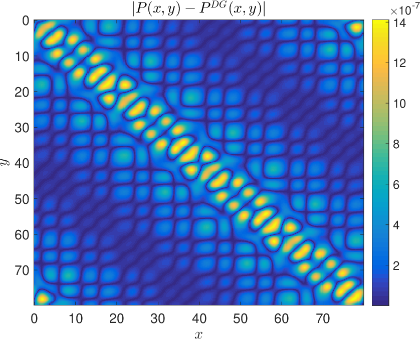
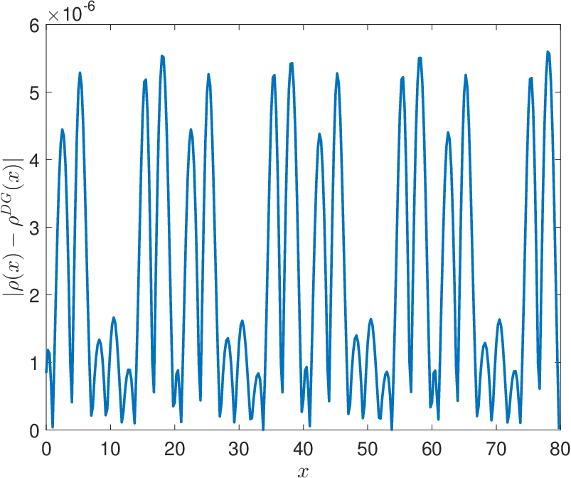
Tab. 6 indicates that the calculation using both the GC-ALB set and the planewave basis set converges within 11 outer SCF iterations to a relative error around , and the number of inner iterations in each outer iteration is comparable in both methods. This indicates that the use of the GC-ALB set does not increase the number of the SCF iterations in the nonlinear setup. The relative error from both methods also behaves similarly throughout the SCF iteration. The spectral projector, as well as electron density defined to be diagonal of the converged projector for both methods are given in Fig. 10. The point-wise relative differences for the projector and the density are provided at the last row of Fig. 10, where the errors are about the same level as that of the relative error in Tab. 6.
5 Conclusion
We developed a new method to construct an efficient basis set to represent the spectral projector of a second order differential operator with reduced degrees of freedom. For a given partition of the global domain into sub-domains called elements, the optimal discontinuous basis set on any element can be given by the singular value decomposition of the matrix row block of the spectral projector associated with the element. Our globally constructed adaptive local basis set (GC-ALB) can efficiently approximate such an optimal basis set in practice. The GC-ALB set can be obtained by only applying a matrix function to a small number of random vectors on the global domain, without the need of any buffer areas to define a series of local problems. The GC-ALB set can be used in the context of the discontinuous Galerkin (DG) framework to approximate the spectral projector on the global domain. When the potential is local, the reduced DG matrix is a block sparse matrix. Hence the evaluation of the matrix representation of the spectral projector can be evaluated using fast methods based on sparse linear algebra operations, such as the pole expansion and selected inversion method (PEXSI) [28, 27], and the purification methods [35, 15]. Our method is also flexible and can be applied to operators with local and nonlocal potentials. We verified the effectiveness of the basis set using one, two and three dimensional linear problems, as well as one-dimensional nonlocal, as well as nonlinear problems resembling Hartree-Fock problems. Numerical results indicate that the GC-ALB set achieve nearly optimal performance in terms of the number of degrees of freedom per element, which reduces both the storage and the computational cost. In the near future, we will explore the usage of the GC-ALB set for Kohn-Sham density functional theory calculations for real materials.
Acknowledgments
L. L. was partially supported by the National Science Foundation under Grant No. DMS-1652330, and by the U.S. Department of Energy under contract number DE-SC0017867, DE-AC02-05CH11231, and the Scientific Discovery through Advanced Computing (SciDAC) program. Y. L. was partially supported by the supported by the National Science Foundation under award DMS-1328230 and the U.S. Department of Energy’s Advanced Scientific Computing Research program under award DE-FC02-13ER26134/DE-SC0009409. We would like to thank Lexing Ying for fruitful discussions.
References
- [1] N. I. Akhiezer, Elements of the theory of elliptic functions, American Mathematical Soc., 1990.
- [2] M. Alemany, M. Jain, L. Kronik, and J. Chelikowsky, Real-space pseudopotential method for computing the electronic properties of periodic systems, Phys. Rev. B, 69 (2004), p. 075101.
- [3] D. G. Anderson, Iterative procedures for nonlinear integral equations, J. Assoc. Comput. Mach., 12 (1965), pp. 547–560.
- [4] D. N. Arnold, An interior penalty finite element method with discontinuous elements, SIAM J. Numer. Anal., 19 (1982), pp. 742 – 760.
- [5] D. N. Arnold, F. Brezzi, B. Cockburn, and L. D. Marini, Unified analysis of discontinuous Galerkin methods for elliptic problems, SIAM J. Numer. Anal., 39 (2002), pp. 1749–1779.
- [6] I. Babuška and J. M. Melenk, The partition of unity method, Int. J. Numer. Meth. Eng., 40 (1997), pp. 727–758.
- [7] A. S. Banerjee, L. Lin, W. Hu, C. Yang, and J. E. Pask, Chebyshev polynomial filtered subspace iteration in the Discontinuous Galerkin method for large-scale electronic structure calculations, J. Chem. Phys., 145 (2016), p. 154101.
- [8] A. D. Becke, Density functional thermochemistry. III. The role of exact exchange, J. Chem. Phys., 98 (1993), p. 5648.
- [9] J.-P. Berrut and L. N. Trefethen, Barycentric Lagrange interpolation, SIAM Rev., 46 (2004), pp. 501–517.
- [10] V. Blum, R. Gehrke, F. Hanke, P. Havu, V. Havu, X. Ren, K. Reuter, and M. Scheffler, Ab initio molecular simulations with numeric atom-centered orbitals, Comput. Phys. Commun., 180 (2009), pp. 2175–2196.
- [11] J. L. Fattebert and J. Bernholc, Towards grid-based O(N) density-functional theory methods: Optimized nonorthogonal orbitals and multigrid acceleration, Phys. Rev. B, 62 (2000), pp. 1713–1722.
- [12] C. J. García-Cervera, Jianfeng Lu, Yulin Xuan, and Weinan E, Linear-scaling subspace-iteration algorithm with optimally localized nonorthogonal wave functions for Kohn-Sham density functional theory, Phys. Rev. B, 79 (2009), p. 115110.
- [13] L. Genovese, A. Neelov, S. Goedecker, T. Deutsch, S. A. Ghasemi, A. Willand, D. Caliste, O. Zilberberg, M. Rayson, A. Bergman, and R. Schneider, Daubechies wavelets as a basis set for density functional pseudopotential calculations, J. Chem. Phys., 129 (2008), p. 014109.
- [14] Paolo Giannozzi, Stefano Baroni, Nicola Bonini, Matteo Calandra, Roberto Car, Carlo Cavazzoni, Davide Ceresoli, Guido L Chiarotti, Matteo Cococcioni, Ismaila Dabo, Andrea Dal Corso, Stefano de Gironcoli, Stefano Fabris, Guido Fratesi, Ralph Gebauer, Uwe Gerstmann, Christos Gougoussis, Anton Kokalj, Michele Lazzeri, Layla Martin-Samos, Nicola Marzari, Francesco Mauri, Riccardo Mazzarello, Stefano Paolini, Alfredo Pasquarello, Lorenzo Paulatto, Carlo Sbraccia, Sandro Scandolo, Gabriele Sclauzero, Ari P Seitsonen, Alexander Smogunov, Paolo Umari, and Renata M Wentzcovitch, QUANTUM ESPRESSO: A modular and open-source software project for quantum simulations of materials, J. Phys.: Condens. Matter, 21 (2009), pp. 395502–395520.
- [15] S. Goedecker, Linear scaling electronic structure methods, Rev. Mod. Phys., 71 (1999), pp. 1085–1123.
- [16] G. H. Golub and C. F. Van Loan, Matrix computations, Johns Hopkins Univ. Press, Baltimore, fourth ed., 2013.
- [17] S. Güttel, E. Polizzi, P. T. P. Tang, and G. Viaud, Zolotarev quadrature rules and load balancing for the FEAST eigensolver, SIAM J. Sci. Comput., 37 (2015), pp. A2100–A2122.
- [18] N. Halko, P.-G. Martinsson, and J. A. Tropp, Finding structure with randomness: Probabilistic algorithms for constructing approximate matrix decompositions, SIAM Rev., 53 (2011), pp. 217–288.
- [19] J. Heyd, G. E. Scuseria, and M. Ernzerhof, Hybrid functionals based on a screened coulomb potential, J. Chem. Phys., 118 (2003), pp. 8207–8215.
- [20] P. Hohenberg and W. Kohn, Inhomogeneous electron gas, Phys. Rev., 136 (1964), pp. B864–B871.
- [21] W. Hu, L. Lin, and C. Yang, DGDFT: A massively parallel method for large scale density functional theory calculations, J. Chem. Phys., 143 (2015), p. 124110.
- [22] A. V. Knyazev, Toward the optimal preconditioned eigensolver: Locally optimal block preconditioned conjugate gradient method, SIAM J. Sci. Comp., 23 (2001), pp. 517–541.
- [23] W. Kohn and L. Sham, Self-consistent equations including exchange and correlation effects, Phys. Rev., 140 (1965), pp. A1133–A1138.
- [24] C. Lanczos, An iteration method for the solution of the eigenvalue problem of linear differential and integral operators, J. Res. Nat. Bur. Stand., 45 (1950), pp. 255–282.
- [25] Y. Li and H. Yang, Spectrum slicing for sparse Hermitian definite matrices based on Zolotarev’s functions, tech. report, 2017.
- [26] L. Lin, Adaptively compressed exchange operator, J. Chem. Theory Comput., 12 (2016), p. 2242.
- [27] L. Lin, M. Chen, C. Yang, and L. He, Accelerating atomic orbital-based electronic structure calculation via pole expansion and selected inversion, J. Phys.: Condens. Matter, 25 (2013), p. 295501.
- [28] L. Lin, J. Lu, L. Ying, R. Car, and W. E, Fast algorithm for extracting the diagonal of the inverse matrix with application to the electronic structure analysis of metallic systems, Comm. Math. Sci., 7 (2009), p. 755.
- [29] L. Lin, J. Lu, L. Ying, and W. E, Adaptive local basis set for Kohn-Sham density functional theory in a discontinuous Galerkin framework I: Total energy calculation, J. Comput. Phys., 231 (2012), pp. 2140–2154.
- [30] , Optimized local basis function for Kohn-Sham density functional theory, J. Chem. Phys., 231 (2012), p. 4515.
- [31] L. Lin and B. Stamm, A posteriori error estimates for discontinuous Galerkin methods using non-polynomial basis functions. Part I: Second order linear PDE, Math. Model. Numer. Anal., 50 (2016), p. 1193.
- [32] , A posteriori error estimates for discontinuous Galerkin methods using non-polynomial basis functions. Part II: Eigenvalue problems, Math. Model. Numer. Anal., (2017, in press).
- [33] L. Lin and C. Yang, Elliptic preconditioner for accelerating self consistent field iteration in Kohn-Sham density functional theory, SIAM J. Sci. Comp., 35 (2013), pp. S277–S298.
- [34] R. Martin, Electronic structure – Basic theory and practical methods, Cambridge Univ. Pr., West Nyack, NY, 2004.
- [35] R. McWeeny, Some recent advances in density matrix theory, Rev. Mod. Phys., 32 (1960), pp. 335–369.
- [36] S. Mohr, L. E. Ratcliff, P. Boulanger, L. Genovese, D. Caliste, T. Deutsch, and S. Goedecker, Daubechies wavelets for linear scaling density functional theory, J. Chem. Phys., 140 (2014), p. 204110.
- [37] P. Motamarri and V. Gavini, Subquadratic-scaling subspace projection method for large-scale Kohn-Sham density functional theory calculations using spectral finite-element discretization, Phys. Rev. B, 90 (2014), p. 115127.
- [38] T. Ozaki, Variationally optimized atomic orbitals for large-scale electronic structures, Phys. Rev. B, 67 (2003), pp. 155108–155112.
- [39] C. C. Paige and M. A Saunders, Solution of sparse indefinite systems of linear equations, SIAM J. Numer. Anal., 12 (1975), pp. 617–629.
- [40] J. E. Pask, B. M. Klein, C. Y. Fong, and P. A. Sterne, Real-space local polynomial basis for solid-state electronic-structure calculations: A finite-element approach, Phys. Rev. B, 59 (1999), p. 12352.
- [41] M. J. Rayson and P. R. Briddon, Highly efficient method for Kohn-Sham density functional calculations of 500–10000 atom systems, Phys. Rev. B, 80 (2009), p. 205104.
- [42] Y. Saad and M. H. Schultz, GMRES: A generalized minimal residual algorithm for solving nonsymmetric linear systems, SIAM J. Sci. Stat. Comput., 7 (1986), pp. 856–869.
- [43] K. Schwarz, P. Blaha, and G. K. H. Madsen, Electronic structure calculations of solids using the WIEN2k package for material sciences, Comput. Phys. Commun., 147 (2002), pp. 71–76.
- [44] C.K. Skylaris, P.D. Haynes, A.A. Mostofi, and M.C. Payne, Introducing ONETEP: Linear-scaling density functional simulations on parallel computers, J. Chem. Phys., 122 (2005), p. 084119.
- [45] J. M. Soler, E. Artacho, J. D. Gale, A. García, J. Junquera, P. Ordejón, and D. Sánchez-Portal, The SIESTA method for ab initio order-N materials simulation, J. Phys.: Condens. Matter, 14 (2002), pp. 2745–2779.
- [46] N. Sukumar and J. E. Pask, Classical and enriched finite element formulations for Bloch-periodic boundary conditions, Int. J. Numer. Meth. Engng., 77 (2009), p. 1121.
- [47] A. Szabo and N.S. Ostlund, Modern quantum chemistry: Introduction to advanced electronic structure theory, McGraw-Hill, New York, 1989.
- [48] M. B. van Gijzen, Y. A. Erlangga, and C. Vuik, Spectral analysis of the discrete Helmholtz operator preconditioned with a shifted Laplacian, SIAM J. Sci. Comput., 29 (2007), pp. 1942–1958.
- [49] G. Zhang, L. Lin, W. Hu, C. Yang, and J. E. Pask, Adaptive local basis set for Kohn–Sham density functional theory in a discontinuous Galerkin framework II: Force, vibration, and molecular dynamics calculations, J. Comput. Phys., 335 (2017), p. 426.
- [50] Y. Zhou, J. R. Chelikowsky, and Y. Saad, Chebyshev-filtered subspace iteration method free of sparse diagonalization for solving the Kohn-Sham equation, J. Comput. Phys., 274 (2014), pp. 770–782.
- [51] Y. Zhou, Y. Saad, M. L. Tiago, and J. R. Chelikowsky, Self-consistent-field calculations using Chebyshev-filtered subspace iteration, J. Comput. Phys., 219 (2006), pp. 172–184.
- [52] E. Zolotarev, Application of elliptic functions to questions of functions deviating least and most from zero, Zap. Imp. Akad. Nauk. St. Petersbg., 30 (1877), pp. 1–59.