Optimal Universal Controllers for Roll Stabilization
Abstract
Roll stabilization is an important problem of ship motion control. This problem becomes especially difficult if the same set of actuators (e.g. a single rudder) has to be used for roll stabilization and heading control of the vessel, so that the roll stabilizing system interferes with the ship autopilot. Finding the “trade-off” between the concurrent goals of accurate vessel steering and roll stabilization usually reduces to an optimization problem, which has to be solved in presence of an unknown wave disturbance. Standard approaches to this problem (loop-shaping, LQG, -control etc.) require to know the spectral density of the disturbance, considered to be a “colored noise”. In this paper, we propose a novel approach to optimal roll stabilization, approximating the disturbance by a polyharmonic signal with known frequencies yet uncertain amplitudes and phase shifts. Linear quadratic optimization problems in presence of polyharmonic disturbances can be solved by means of the theory of universal controllers developed by V.A. Yakubovich. An optimal universal controller delivers the optimal solution for any uncertain amplitudes and phases. Using Marine Systems Simulator (MSS) Toolbox that provides a realistic vessel’s model, we compare our design method with classical approaches to optimal roll stabilization. Among three controllers providing the same quality of yaw steering, OUC stabilizes the roll motion most efficiently.
Keywords:
Roll stabilization, ship motion control, ship maneuvering, optimal control1 Introduction
Roll stabilization is a classical problem in ship motion control (Fossen, 1994; Perez, 2006; Perez and Blanke, 2012). Passive roll stabilization can be provided by special equipment such as bilge keels, water-tanks and moving weights (Perez, 2006; Perez and Blanke, 2012; Marzouk and Nayfeh, 2009); however, these devices cannot be easily adapted to the unsteady environment and the changing wave’s spectrum. This limitation can be overcome by active (controlled) roll stabilization, which can be provided by gyroscopic stabilizers, stabilizing fins and/or actuators (rudders and thrusters) used for the vessel’s steering. This is illustrated by the rudder roll stabilization (RRS), proposed originally for a vessels equipped with a single rudder (Cowley and Lambert, 1972; Carley, 1975; Lloyd, 1975). Since fins, rudders and thrusters affect both yaw and roll motion of the vessel, the roll stabilization controller should be integrated with the heading controller (autopilot). These control systems can share some actuators and pursue concurrent goals of roll stabilization control and course steering.
A vessel’s coupled yaw-roll motion can be modeled by a dynamical system, whose inputs are the rudder’s and fins’ angles and whose outputs stand for the ship’s heading and roll. After linearizing this model, classical methods of linear control, e.g. loop shaping and Quantitative Feedback Theory (Cowley and Lambert, 1972; Carley, 1975; Horowitz and Sidi, 1978; Blanke and Christensen, 1993; Hearns and Blanke, 1998) can be applied to stabilize yaw and roll motion. To cope with nonlinearities, methods of feedback linearization and sliding mode control can be used (Lauvdal and Fossen, 1997; Liu et al., 2016). For vessels equipped with fin stabilizers, classical methods usually decouple the roll motion from the yaw motion (Surendran et al., 2007; Hinostroza et al., 2015). However, ignoring internal cross-couplings often reduces the overall performance (Carley and Duberley, 1972).
The roll dynamics of a vessel appear to be non-minimum phase, leading thus to the fundamental limitation (Carley, 1975; Goodwin et al., 2000): a controller stabilizing the vessel’s heading cannot fully attenuate the wave-induced roll oscillations. A natural question arises, namely which level of the roll oscillation stabilization can be provided without deteriorating the yaw control. Mathematically, the latter goal is usually formulated as optimality of a special performance index, which penalizes the time-averaged steering error, roll angle and the control effort. Besides the control input, such a functional implicitly depends on the uncertain wave disturbance that affects the ship’s motion. Unlike the aforementioned stabilization techniques, optimization-based algorithms assume that some model of the disturbance is known. Most typically, the wave-induced motion is approximated by either a “colored noise” or a random polyharmonic signal (Perez and Blanke, 2012; Fossen, 1994).
The wave model of the first type approximates the wave disturbance by the output of some low-pass shaping filter, fed by a white noise. This approach, prevailing in the literature, reduces roll stabilization control design to standard methods of optimal controller synthesis, such as the linear-quadratic Gaussian (LQG) control (van der Klugt, 1987; van Amerongen et al., 1990), control (Sharif et al., 1995; Blanke et al., 2000; Crossland, 2003; Stoustrup et al., 1994) and model-predictive control (MPC) (Perez, 2006). As usual in stochastic and minimax control, optimal controllers do not deliver optimal solutions for any specific realization of the stochastic disturbance, providing optimality either “on average” (in the sense of expectation) or in the “worst-case” scenario. Another downside of the mentioned methods is the necessity to estimate the spectral density of the wave motion.
An alternative “discrete” model of the wave motion, often used in marine engineering (Perez, 2006; Nicolau et al., 2005; Longuet-Higgins, 1963), approximates the wave motion by the sum of sinusoids with known frequencies, where the constant amplitudes are obtained via sampling of the spectral density and random phase shifts are uniformly distributed in in order to get different realizations. For this model of the wave disturbance and linearized vessel’s yaw-roll dynamics, the optimal roll stabilization may be considered as a linear-quadratic optimization problem, where the control system is affected by a partially uncertain polyharmonic signal. A relevant extension of the classical LQR control to cope with such problems has been developed in (Yakubovich, 1995; Lindquist and Yakubovich, 1997; Lindquist and Yakubovich, 1999; Proskurnikov and Yakubovich, 2006; Proskurnikov and Yakubovich, 2012; Proskurnikov, 2015). It appears that (under natural assumptions) an optimal universal controller (OUC) exists, which is independent of the uncertain signal’s parameters, delivers the optimal process for arbitrary values of these parameters. Furthermore, the OUC can be found in the class of linear stabilizing controllers; a convenient parametrization of such OUCs has been found (Yakubovich, 1995).
In this paper, we apply Yakubovich’s theory of OUC to the problem of optimal roll stabilization. This paper extends our previous work (Kapitanyuk et al., 2016), which considered a simplified model of the vessel with a single rudder and no stabilizing fins. We illustrate the efficiency of OUCs in the optimal roll stabilization problem and compare it with classical controllers by using numerical simulations that utilize the “benchmark” vessel’s model from (Perez, 2006). The OUC theory provides a method for combined fin-rudder stabilization control design, avoiding the undesired counteraction between different actuators and improving the resulting efficiency of the control system. Unlike the usual LQR (Perez and Blanke, 2012), the OUC does need to measure the full state vector and provides optimality for any polyharmonic signal from the specified class; to find OUC, one does not need to solve the Riccati equation. Unlike LQG and approaches, the OUC design does not require one to know the spectral density of the wave motion (or, equivalently, the structure of the shaping filter). The OUC depends only on the fixed wave’s frequencies and ensures optimality of the cost functional for any realization of the random disturbance.
The paper is organized as follows. In Section 2, mathematical models of the vessel’s motion and wave disturbances are considered. In Section 3 the theory of OUC in general problems of linear-quadratic optimization with uncertain disturbances is introduced. In Section 4, we apply this theory to design an optimal roll stabilization controller, whose performance is studied numerically in Section 5.
2 Mathematical models
We first introduce mathematical models of the ship’s yaw-roll motion and the wave disturbances.
2.1 The vessel’s motion
The movements of a marine vessel (as a rigid body) have six degrees of freedom. The standard 6-DoF mathematical model can be found in (Perez and Blanke, 2012; Fossen, 1994). However, it is more convenient to use a simplified reduced-order model (van Amerongen et al., 1990; Fossen, 1994; Perez, 2006), which is derived (see details in A) under two simplifying assumptions: 1)the effects of the pitch and heave motion of the vessel on its surge, sway, roll and yaw dynamics are negligibile; 2) the vessel’s speed is changing slowly relative to the remaining coordinates. Under these assumptions, the yaw and the roll controllers can be designed for a simplified linearized model.
In the original papers on rudder roll stabilization (Cowley and Lambert, 1972; Lloyd, 1975), the simplest configuration of the vessel with one rudder has been considered, whose angle is the single control input of the system. In general, the vessel can be equipped with multiple actuators (rudders, azimuth and tunnel thrusters, waterjets etc.); however, for the sake of autopilot and roll stabilization control design they are usually replaced by an equivalent “virtual rudder”, whose “angle” stands for the scaled rotating yaw moment, distributed among the actuators by a separate control allocation system (Johansen et al., 2008). In addition to this, we allow the vessel to have synchronized stabilizing fins, whose angle serves as the second control.
Denoting the rudder, the fin, the roll and the yaw (or heading) angles by, respectively, , , and (Fig. 1), the reduced-order vessel’s model has the structure illustrated in Fig. 2. The system is affected by the environmental disturbance, represented by its roll and yaw components11 1 For clarity, in this paper we consider the “motion superposition” model (Perez, 2006), where the disturbance is modeled as an uncertain displacement from the original trajectory of the vessel. An alternative approach, referred to as the “force superposition” (Perez, 2006), treats the disturbance as an additional force, acting on the ship’s hull. , . The transfer functions from and to and , denoted by , , and , respectively, are as follows (Perez, 2006, Sect. 8.2)
| (1) |
where , , and are constants. Notice that this model takes into account coupling between the sway, roll and yaw motions of the vessel. Ignoring the cross-coupling between yaw and roll, the model can be further reduced (Fossen, 1994, Section 9.1.1).
Along with the transfer function, one can introduce the state-space model of the system
| (2) | ||||
Here the vessel’s reduced state vector consist of the roll angle , the roll rate , the yaw angle , the yaw rate and the sway velocity . The disturbance stands for the wave-induced motion of the vessel. The vector stands for the system’s output, whose components and are measured, respectively, by a vertical reference unit (VRU) sensor (Balloch, 1998) and a gyro or GPS compass and the control input is presented by the vector .
The explicit derivation of the matrices is given in A. It should be noticed that the controller design, in fact, does not use their explicit values and requires only the knowledge of the transfer functions (1).


2.2 The disturbance model
The environmental disturbances, influencing a marine craft’s motion, are due to the waves, the wind and the current. The fast oscillations in the roll and the heading angles are mainly caused by the waves, whereas the current and the wind are changing much more slowly and their effect is usually modeled as a constant roll angle and stationary heading deviation. Henceforth, the disturbance stands for the wave-induced motion only. In this paper, we use a polyharmonic approximation of this motion (Perez and Blanke, 2012; Fossen, 1994)
| (3) |
Here the spectrum is known. The special case corresponds to the model of regular waves; however, a real state of the sea is best described by a random or irregular wave model. This stochastic process can be approximated by the model (3) with being sufficiently large. The constant amplitudes and are obtained via sampling the spectral density with a small enough step to ensure that the fundamental period of the finite sum of sinusoidal components is longer than the desired duration of the simulation. The random phase shifts and used to generate different realizations of the stochastic process are uniformly distributed in . Although the model (3) of irregular waves can describe a sea state quite accurately, the direct use of it in the control design is difficult due to the high dimension. The better strategy is to consider a few “dominating” frequencies corresponding to the peaks of the spectral density. In general, the localization and the shape of the spectral density highly depend on many parameters of motion such as the average speed of the vessel, sailing conditions and a frequency response of the vessel’s hull; however, these “dominating” frequencies can be efficiently estimated in real time, see e.g. (Belleter et al., 2015; Bobtsov et al., 2012; Fedele and Ferrise, 2012; Hou, 2012) and references therein. For simplicity and clarity of presentation, we proceed to assume that the number and the values of such frequencies are known.
It should be noted that in the existing control literature the wave motion is usually approximated by the “colored noise”, that is, the output from a low-pass shaping filter fed by the white noise signal. The simplest approximation for the shaping filter’s transfer function (that is, the wave spectrum), is
| (4) |
Here the constant determines the wave strength, is the encounter frequency and is the damping ratio (Perez and Blanke, 2012). Unlike our approach, using only the information about the frequencies, the existing approaches, as discussed in Introduction, typically use all parameters of the transfer function , whose identification is a self-standing non-trivial problem. As discussed in (Perez and Blanke, 2012, Sect. 2.5), the shaping filter representation of the wave is primarily used in stochastic control, which is convenient for methods exploiting spectral factorization of the wave disturbance, while the more precise nolinear multi-sine model is commonly used in naval architecture.
3 Linear-quadratic optimization in presence of uncertain polyharmonic signals
In this section, the basic ideas of the theory of OUC are given for the reader’s convenience, following the survey paper (Proskurnikov, 2015). The concept of universal controller dates back to early works on “signal invariance”, or disturbance decoupling in control systems, see e.g. the survey in Proskurnikov and Yakubovich (2003a); Proskurnikov and Yakubovich (2003b).
We start with introducing some notation. The set of complex matrices is denoted by . The Hermitian complex-conjugate transpose of a matrix is denoted by . We use to denote the imaginary unit. The real part of a number is denoted by .
3.1 A family of uncertain optimization problems
Consider a linear time-invariant MIMO system, influenced by an exogenous signal
| (5) |
Here stand for, respectively, the state vector, the control and the observed output. The signal is a polyharmonic process with known spectrum
| (6) |
whose complex amplitudes (absorbing also the phase shifts) are uncertain. The components of this exogenous signal may include disturbances, measurement noises and reference signals.
In presence of the oscillatory disturbance (6), the solutions of (5) do not vanish at infinity. The goal of control is to guarantee boundedness of the solution and its optimality in the sense of the following quadratic performance index
| (7) |
Here is a quadratic form, which is assumed to be non-negative definite . Considering the integrand in (7) as a measure of the solution’s “energy”, its average value can be thought of as the solution’s average “power”. Formally, the control goal can be formulated as follows
| (8) |
In fact, (8) defines an infinite family of optimization problems, corresponding to different choices of the amplitudes . Obviously, the set of optimal processes also depends on the amplitudes and hence cannot be found explicitly. Nevertheless, it can be shown that an optimal universal controller (OUC) exists that provides an optimal process for any uncertain amplitudes , solving thus the whole family of optimization problems (8).
3.2 A class of linear OUC
Although the existence of OUCs may seem exceptional, such controllers exist under rather mild assumptions on the system and the cost functional.
We assume that the system (5) is stable, that is, whenever . If the system is stabilizable and detectable, one may always augment it with an observer-based stabilizing controller, so the stability assumption can be adopted without loss of generality.
Let stand for the matrix of the quadratic form and be the matrix of the quadratic form , that is,
| (9) | ||||
where are matrices of appropriate dimensions. We introduce the rational complex-valued matrix as follows
and assume that the frequency-domain condition holds
| (10) |
The condition (10) is a standard solvability condition for classical LQR problems, providing the existence of the stabilizing solution to the Riccati equation (Anderson and Moore, 1990). It always holds when is positively definite, which is a natural assumption in practice. The condition(10) cannot be discarded and, moreover, its “strong” violation in the sense that for some and implies22 2 For a similar discrete-time optimization problem, the proof is available in (Lindquist and Yakubovich, 1999), and the continuous-time case is considered in the same way. the ill-posedness of the problem (8): for any signal (6).
Under non-restrictive assumptions, the OUC exists and can be found among linear controllers
| (11) |
where and stand for matrix polynomials; the matrix is square and . The relevant result is given by the following theorem.
Theorem 1
(Proskurnikov, 2015) Let the system (5) be stable and the inequality (10) hold. Then the linear controller (11) is an OUC for the family of problems (8) if the following two conditions hold
- 1.
the closed-loop systems is stable, that is,
(12) - 2.
the closed-loop transfer function from to satisfies the interpolation equations
(13) where the constant matrices are as follows
Note that, unlike the classical LQR problem, where the optimal controller is uniquely defined from the Riccati equation, the OUC in the problem (8) is not unique; to find it, one need not solve Riccati equations. We will use Theorem 1 in a special situation, where depends only on the output and the control, i.e. admits the decomposition
| (14) |
where . In this situation, one has
| (15) |
Here and stand for the open-loop transfer functions from respectively and to
Recalling that is a Hurwitz matrix, it can be shown that the closed-loop system is stabilized by the controller (11), whose coefficients are as follows
| (16) |
Here is a matrix polynomial and is a scalar Hurwitz polynomial with . Such a controller is “feasible” in the sense that its transfer matrix , as well as the closed-loop system’s transfer matrices from to , are proper. For the controller (11),(16), one obtains
| (17) |
and the interpolation constraints (13) boil down to
| (18) |
The constraints (18) can be satisfied when
| (19) |
Here is the open-loop transfer matrix from to . The conditions (19) typically hold when . Furthermore, if (19) holds, the coefficients of and can be chosen as continuous functions of , so that the controller is robust to small deviations in the spectrum . Choosing an arbitrary Hurwitz polynomial of degree , one needs to find the matrix polynomial with , satisfying the conditions
| (20) |
Separating the real and imaginary parts, one obtains equations for real coefficients of .
It appears that any OUC (11) is equivalent, in some sense (Yakubovich, 1995; Proskurnikov, 2015), to the controller (16) with some polynomials , satisfying the interpolation constraints (18).
Remark 1
Note that the controller (16) in fact does not depend on the state-space model (5), involving only the system’s characteristic polynomial and the open-loop transfer function from to (Fig. 3). In the case where depends only on and , the interpolation conditions (18) also involve only the values of and rather than the whole state model (5). Hence, in this special situation, the design of OUC requires only the knowledge of , and , which are independent of the minimal state-space realization.

Remark 2
In general, one has a lot of freedom in choosing the coefficients of , and their “optimal” choice remains an important research topic as a subject of ongoing research. In practice, the polyharmonic model of the disturbance is usually imprecise: the signal contains frequencies other than (whose amplitudes are sufficiently small). Fig. 3 suggests that, ideally, the OUC’s transfer function should have a sufficiently narrow bandpass, containing the frequencies in order to damp these unmodeled spectrum. Although this requirement is not very formal, it can be used for practical tuning of the OUC’s parameters.
Remark 3
As discussed in (Lindquist and Yakubovich, 1999), the important property of the OUC (11) is its robustness against small changes in the frequencies , whereas the straightforward LQR-based design leads to a controller that is formally optimal yet non-robust to deviations in spectrum. The results from (Lindquist and Yakubovich, 1999) deal with discrete-time systems, but this robustness property is retained by the continuous-time OUC (11).
4 Optimal Universal Roll Stabilization Controllers
In this section, we reduce the optimal roll stabilization problem to a special case of the problem (8). The cost functional will depend only on the control effort and output. In view of Remark 1, in this situation one does not need to know a special state-space representation of the open-loop system, requiring only its characteristic polynomial and transfer matrices . In this sense, an optimal controller can be designed in the frequency domain.
We assume that the vessel’s heading is stabilized by a known autopilot (Fig. 4). Behind this statement, there are two practical considerations. First of all, it allows splitting of the adjustment procedure for a motion control system on the vessel in two sequential stages: the independent tuning of an autopilot and the following design of the roll stabilization controller. The second reason is the flexibility and the modularity; the roll stabilization system may be supplied by a manufacturer of the equipment such as high-performance rudders or active fins independent of the development of the autopilot, which is in itself a challenging task. The autopilot design problem has been thoroughly studied in the literature (Fossen, 1994; Perez, 2006; Nicolau et al., 2005; Veremey, 2014) and is beyond the scope of this paper. Furthermore, we assume that the roll stabilization system is aware of the measured heading of the vessel and the constant heading setpoint . In practice, can be a function of time, e.g. when autopilot steers the vessel along a curvilinear path. However, these dynamics are much slower than the ship’s roll motion, and hence are neglected in the roll stabilization system design. The deviation among them (heading error) , along with the roll stabilization error are the inputs to the roll stabilization system (Fig. 4). Mathematically,
The rudder angle is the sum of the autopilot’s and the roll stabilization controller’s commands (Fig. 4), denoted respectively by and . The fin angle is used as the second control input . Denoting the autopilot’s transfer function by , one has

The yaw-roll dynamics of the vessel, closed by the autopilot, are represented by the input-output model
| (21) |
Here are the polyharmonic components of the wave-induced motion (3). Considering as a harmonic signal of zero frequency, is a special case of (6) with and , where , are the wave frequencies from (6) and . The transfer functions depend on the autopilot’s transfer function (from to ) and the functions from (1). The exact formulas for are derived in B and it can be easily seen from these formulas that (19) always holds for any wave .
The cost functional penalizes the mean square values of the following three variables (i) the roll displacement (), (ii) the heading deviation (), and (iii) the control effort . Denoting the corresponding penalty weights by , we introduce the quadratic cost functional as follows
| (22) |
The Hermitian form can be represented in the form (14), where is defined by
The matrix function and the matrices are defined by (15); since .
This formalization of the RRS problem makes it possible to apply the theory of optimal universal controllers, discussed in the previous section. To design OUC (11) with the coefficients (16), one has to choose to be a scalar Hurwitz polynomial with , whereas is a matrix polynomial that satisfies (18). By fixing and splitting the real and imaginary parts in the interpolation condition (18), one obtains a pair of real-valued matrix equations for the coefficients of . The only exception is : since , the equation (18) is real-valued. Hence we get equations for the coefficients of the polynomial . To satisfy them, the polynomial should have real-valued coefficients, i.e. it suffices to choose and .
The just described algorithm to design an OUC for the roll stabilization problem can be summarized as follows:
For the detailed derivation of the OUC controller one may represent the transfer functions (1) as follows
| (23) |
In order to stabilize the vessel’s heading, the autopilot controller is chosen to be
| (24) |
The application of this procedure to a specific vessel’s model is illustrated in the next section.
5 Numerical simulation
In this section we consider a numerical example to illustrate the proposed approach.
5.1 Vessel’s motion and wave disturbance
To design the linear controllers, we consider the vessel’s 4-DoF (surge, sway, roll and yaw) model from (Perez, 2006, Appendix B). This maneuvering model of a multipurpose naval vessel is implemented in the Marine Systems Simulator (MSS) Toolbox (Fossen and Perez, 2004) in our numerical simulations. The vessel has one rudder and two synchronous fins. Linearizing the model at the speed m/s, the coefficients of the transfer functions (23) are as follows (Perez, 2006, Appendix B)
For this simulation we assume that the stabilizing autopilot (24) has the following form
Whereas the controller design is based on this linearized model, our simulations take into account the nonlinear dynamics of the rudder’s and fins’ steering machines (Perez, 2006, 5.6) with the maximal angles degrees (rudder) and degrees (fins) and the maximal rates degree/s and degree/s respectively. (Perez, 2006, Appendix B.4).
To cope with saturations, we use the heuristical approach, called the automatic gain control (AGC) (van der Klugt, 1987; Lauvdal and Fossen, 1998) that decreases the actuator command in a smart way to ensure that saturation (of the actuator angle or rate) never occurs. In Fig. 5 we compare the commands from our OUC (whose design will be specified in Subsection 5.3) before and after the AGC algorithm. The rudder is not saturated, in this case the command remains unchanged. The fin angle’s saturation is prevented by AGC.


To obtain the proper time series of the polyharmonic approximation of the irregular wave (3) we use the methodology presented in (Perez and Blanke, 2012, Sect. 4.2.5). The resulting realization is obtained for the long-crested irregular sea in beam seas. The response amplitude operator has been taken from (Perez and Blanke, 2012, Table B.9.), where the number of sinusoidal components is . We consider the JONSWAP spectrum (Fossen, 1994, Section 4.2.1), which is characterized by two parameters: the significant wave height and the peak value of the spectrum (peak frequency). We consider two different significant wave heights (m and m) and three different peak values ( rad/s, rad/s, rad/s). Also, we compare the controllers’ behavior at three different speeds: m/s (the linearization point of the model at which the controller is designed), m/s (medium speed) and m/s (low speed at which the rudders and fins are limited with small inflow velocity). In total, we consider 6 different scenarios (Table 1). The power spectra are shown in Fig. 6a-d).
We use “rough” approximations of the signal (3) taking only one “dominating” sinusoidal components. For the frequencies of the sinusoidal signal, we choose rad/s and rad/s. To evaluate the robustness of OUC against unspecified harmonics, in Case 6 we consider the peak frequency rad/s which is different from and .


| Case | Vessel speed, m/s | Wave Height, m | Peak value, rad/s |
| 1 | 8 | 3 | 1.15 |
| 2 | 5 | 3 | 1.15 |
| 3 | 1 | 3 | 1.15 |
| 4 | 8 | 1.5 | 1.15 |
| 5 | 8 | 3 | 0.5 |
| 6 | 8 | 3 | 0.8 |
5.2 The standard controllers
We compare the OUC with two other types of linear controllers. The first of these controllers is the classical LQR controller (Fossen, 1994, Appendix D), designed to optimize the cost function
| (25) |
in the absence of disturbances. We choose the parameters , , , .
The conventional loop shaping controller (van Amerongen et al., 1990) has been chosen as another algorithm for comparison. This method ignores the yaw dynamics, working directly with the transfer function (see B). For the known dominating frequency of the disturbance, we select the structure of the notch filter centered at that point to damp the frequencies around it. The controller takes the following form
5.3 The OUC design
The coefficients of the cost functional (22) are chosen as , , and . It should be noted that, in spite of similar cost functions, the behaviors of the two controllers are very different. Actually, the cost function (25) is in principle finite only for the disturbances vanishing as , and its optimality for does not guarantee any optimal performance for the polyharmonic disturbance. For this reason, the choice of the coefficients is a delicate issue. We have tuned them in such a way that the LQR and OUC provide (approximately) same quality of course keeping (see the heading errors in Table 3).
In the design procedure from the previous section, we should choose the Hurwitz polynomial of the order . The polynomial is chosen as follows
| (26) |
Here , , are the frequencies of the wave disturbance, , and
is the characteristic polynomial of the closed-loop system, which corresponds to the LQR controller described above. The reasons to choose this polynomial are discussed below in Subsection 5.5.
5.4 Simulation results


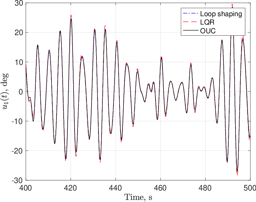
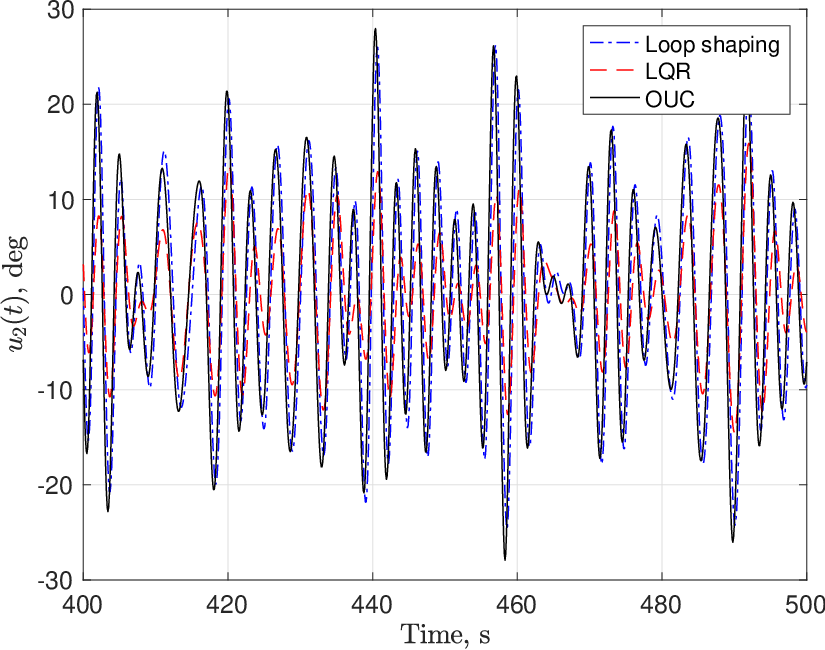


Figs. 7–13 the results of simulation in Cases 1-6 are presented. The simulation time is 500s, in Figs. 7–12 we zoom the time window 400-500s in order to simplify viewing. Fig. 13 shows the dynamics of roll angle for all 6 cases over the whole period of 500s. As has been mentioned, we always combine the controllers with the AGC algorithm.


The standard deviations of roll angle and heading errors are summarized in Tables 2, 3 respectively.
| Case | No control | OUC | LQR | Loop Shaping |
|---|---|---|---|---|
| 1 | 6.2048 | 1.4402 | 3.0443 | 3.2640 |
| 2 | 5.6845 | 2.6524 | 3.7840 | 4.6454 |
| 3 | 5.0869 | 4.8803 | 4.9800 | 5.1226 |
| 4 | 3.5884 | 0.7313 | 1.7237 | 1.7790 |
| 5 | 3.6071 | 1.5213 | 2.0867 | 1.7539 |
| 6 | 4.7570 | 1.8683 | 2.5839 | 2.3128 |
| Case | No control | OUC | LQR | Loop Shaping |
|---|---|---|---|---|
| 1 | 1.0746 | 1.0040 | 1.0202 | 1.0268 |
| 2 | 1.0788 | 1.0532 | 1.0617 | 1.0977 |
| 3 | 1.0169 | 1.0244 | 1.0186 | 1.0196 |
| 4 | 0.6076 | 0.5644 | 0.5747 | 0.5780 |
| 5 | 0.5894 | 0.5541 | 0.5574 | 0.5643 |
| 6 | 0.7959 | 0.7501 | 0.7551 | 0.7638 |
Notice that in Case 3 (the speed is too small) all controllers are equally inefficient since the performance of rudders and fins is very limited. In all other cases, OUC demonstrates smaller average roll than the remaining controllers providing a comparable yaw error. Notice that this also holds in Case 6, although the actual peak frequency of the signal is different from the nominal frequencies of the wave disturbances . The main disadvantage of the LQR is the lack of knowledge about the structure of the disturbance signal. The LQR controller shows better performance than loop shaping in Cases 1-4, because it efficiently damps the ship roll natural (resonance) frequency of the vessel (Perez and Blanke, 2012) (s), which is very close to the peak frequency of the wave disturbance. In Cases 5 and 6, the significant energy of the spectrum is beyond the vicinity of resonance frequency, for this reason, the performance of the simple loop-shaping controller is better.
5.5 Choice of the polynomial and its influence on the closed-loop system
Mathematically, every choice of the scalar polynomial is feasible (provided that it has a sufficiently large degree and is Hurwitz). In practice, its choice influences the characteristics of the closed-loop system since the closed-loop transfer functions from the disturbance to the, respectively, control and the output are
Here and are the stable open-loop transfer functions, independent of the choice of the controller. Hence, the choice of the determines, first, the stable poles of the closed-loop system and, second, its frequency-domain characteristics. The interpolation conditions provide optimal attenuation of the spectrum in a small vicinity of the nominal frequencies . As stated in Remark 2, attenuation of the disturbance frequencies beyond this vicinity is most critical for the overall system performance.
The influence of on the closed-loop system is illustrated in Fig. 14. The latter figure shows the magnitude Bode plots of the functions and (the influence of roll disturbance on the roll angle and rudder angle), corresponding to the polynomial with from (26) and . Here plays the role of the system’s sensitivity. The empirical observation shows that, as one decreases (the system becomes “slower”, or less sensitive), the performance with respect to roll angle deteriorates (in particular, the passband becomes wider), whereas increase in leads to better stabilization. At the same time, large values of correspond to excessive use of the actuators, whereas smaller values of make their dynamics more smooth.


The “optimal” assignment of closed-loop system’s poles and shaping the transfer functions of the closed-loop system are long-standing problems in control theory (Franklin et al., 1981). The denominator of the closed-loop transfer function can be decomposed into the product
where are the so-called natural frequencies, are called damping ratios and are called time constants (Franklin et al., 1981, Chapter 6). Unlike the classical situation, the numerator of the transfer function depends on due to the interpolation constraints (19); also, the order of this transfer function () has to be sufficiently large in order to satisfy the interpolation constraints. In spite of this, the standard recommendations on the pole placement (Franklin et al., 1981), applied to the choice of , give a satisfactory result, as demonstrated by simulations in Section 5.4. One of these recommendations is to place the poles of the closed-loop system by using a standard LQR procedure. Since we are comparing our controller’s behaviors with a specified LQR controller, it is natural to assign the corresponding closed-loop system’s poles (zeros of ) to be the roots of . To attenuate frequencies beyond , and , we also include the two Butterworth polynomials , and an additional multiplier . The value of is chosen in order to provide the attenuation of the disturbance in the frequency band rad/s, which contains 93% of the roll disturbance energy. Also, we renormalize to set its leading coefficient to . This leads us to the polynomial from (26).
6 Conclusions and future work
In this paper, we offer a novel approach to the design of the roll stabilization system for marine vessels, based on the idea of optimal universal controllers (OUC). Unlike the existing approaches, such a controller does not require the full information about the wave’s spectral density, but only the knowledge of its dominant frequencies. A topic of ongoing research is to employ adaptive control methods to enable the controller’s functioning in the fully uncertain environment. In particular, combining the roll stabilization controller with an estimator of the dominating encounter wave frequencies (Bobtsov et al., 2012; Belleter et al., 2015), one can adjust the coefficients of the OUC controller “on the fly”.
In our simulations, the OUC has been enhanced by an automatic gain controller (AGC) (van Amerongen et al., 1990; van der Klugt, 1987) preventing saturation of actuators. It could also be used with alternative gain scheduling techniques, e.g. time-varying gain reduction (Lauvdal and Fossen, 1998) or, more generally, advanced control allocation methods taking into account nonlinear dynamics of actuators (Zaccarian, 2009; Johansen and Fossen, 2013). Mathematical analysis of the resulting nonlinear systems remains, however, a non-trivial problem for future research.
Another limitation that can be relaxed is the fixed cruising speed of the vessel (determining the point of linearization, see A). Our simulation (Section 5.3) shows that the OUC controller is quite robust to the change of speed, although the optimality of the cost function is no longer guaranteed. For vessel’s maneuvers at a non-constant speed, more sophisticated controllers can be designed that are based on the paradigm of gain scheduling (Rugh and Shamma, 2000). Note however that the choice of a specific procedure allowing to redesign a linear fixed-speed controller into a nonlinear controller, applicable for non-constant speed, remains a non-trivial open problem. Also, such a redesign should be applied not only to RRS system, but also to the ship’s autopilot.
Appendix A Linearized 4-DoF vessel motion model
A ship in a seaway moves in 6-DoF: three translation displacements (surge, sway and heave) define the location and three angular displacements (roll, pitch and yaw) define the attitude. In traditional maneuvering problems (such as e.g. course-keeping), normally a 3-DoF model (surge-sway-yaw) is considered. However, to consider the roll stabilization problem, one needs a 4-DoF model that includes the roll motion. In this paper, we use the Christensen and Blanke model (Fossen, 1994, Section 9.1.3). The following equations of motion are valid when the body-fixed axes correspond to the longitudinal, lateral and normal directions:
where m is the mass of the ship; , , are the coordinates of the ship’s center of gravity with respect to the body frame; and are the corresponding diagonal components of the inertia tensor with respect to the body frame; and are the surge and sway velocities; and are the roll and yaw rates. The total vector of forces given with respect to the body frame can be decomposed as
where , , and stand for hydrodynamic, hydrostatic, actuators (fins and rudders) and propulsion forces and moments respectively.
It is usually assumed that the propulsion forces are compensated by the hydrodynamic resistance of the ship’s hull and the surge acceleration is very small, that is, and , where is the service speed of the vessel. This leads to a simplified model to the following form:
| (27) |
where, by definition,
where is the roll angle, is the yaw angle; , and stand for the hydrodynamic derivative (Perez, 2006) of the sway force, roll moment and yaw moment with respect to term; , and are the nonlinear hydrodynamic forces that are found from
where is the water density, is the acceleration of free fall, is the so-called roll righting arm (Perez, 2006), and is is the displaced volume.
Assuming that the changes of roll and yaw angles are small one can linearize the model (27) around the equilibrium point , , , , and , i.e. the vessel is moving straight with the constant speed. That bring us to the following linear model:
where the coefficients are found from (28) and
where
are the resulting hydrodynamic forces induced on the rudder and the fins respectively; are respectively the longitudinal and vertical distances from the center of gravity(CG) to the rudder, is the fins tilt angle defined in the aft view, is the fin roll arm, is a longitudinal distance from the CG to the fin’s center of pressure; and are the lift characteristics for the rudder and fins respectively, and stand for to the rudder and fins areas.
| (28) |
Appendix B Transfer matrices of the ship-autopilot system
In this section we are going to present the transformation procedure on how to obtain the models in equations (21) based on the general dynamics of the vessel described by the transfer function
The observed outputs of the system are
where is the heading setpoint. We introduce the two control inputs as follows
where is the autopilot’s transfer function, stabilizing the vessel’s yaw motion. Putting the equations together, one arrives at the following
Assuming that the autopilot stabilizes the yaw loop i.e. this yields
where
Recalling that
the transfer matrices from and respectively to are given by
References
- Anderson and Moore (1990) Anderson, B. D. O., Moore, J. B., 1990. Optimal Control: Linear Quadratic Methods. Prentice-Hall, Inc., Upper Saddle River, NJ, USA.
- Balloch (1998) Balloch, R., 1998. Attitude sensors for DP. In: Proc. Dynamic Positioning Conf. Houston, TX, USA.
- Belleter et al. (2015) Belleter, D. J., Galeazzi, R., Fossen, T. I., 2015. Experimental verification of a global exponential stable nonlinear wave encounter frequency estimator. Ocean Engineering 97, 48 – 56.
- Blanke et al. (2000) Blanke, M., Adrian, J., Larsen, K.-E., Bentsen, J., 2000. Rudder roll damping in coastal region sea conditions. In: Proc. 5th IFAC Conference on Manoeuvring and Control of Marine Craft (MCMC). Aalborg, Denmark, pp. 30–44.
- Blanke and Christensen (1993) Blanke, M., Christensen, A. C., 1993. Rudder-roll damping autopilot robustness to sway-yaw-roll couplings. 10th Ship Control Systems Symposium, Ottawa 25-29 Oct. 1993.
- Bobtsov et al. (2012) Bobtsov, A. A., Efimov, D., Pyrkin, A. A., Zolghadri, A., Sept 2012. Switched algorithm for frequency estimation with noise rejection. IEEE Transactions on Automatic Control 57 (9), 2400–2404.
- Carley and Duberley (1972) Carley, J., Duberley, A., 1972. Design considerations for optimum ship motion control. In: Proceedings of 3rd Ship Control Systems Symposium, Volume-C. Bath, UK.
- Carley (1975) Carley, J. B., 1975. Feasibility study of steering and stabilising by rudder. In: Proc. 4th Ship control system symposium. The Hague, The Netherlands.
- Cowley and Lambert (1972) Cowley, W., Lambert, T., 1972. The use of the rudder as a roll stabiliser. In: Proc. 3rd Ship Control Syst. Symp. Bath, UK.
- Crossland (2003) Crossland, P., 2003. The effect of roll-stabilisation controllers on warship operational performance. Control Engineering Practice 11 (4), 423 – 431.
- Fedele and Ferrise (2012) Fedele, G., Ferrise, A., 2012. Non adaptive second-order generalized integrator for identification of a biased sinusoidal signal. IEEE Trans. Autom. Control 57 (7), 1838–1842.
- Fossen (1994) Fossen, T., 1994. Guidance and control of ocean vehicles. Wiley.
- Fossen and Perez (2004) Fossen, T. I., Perez, T., 2004. Marine systems simulator (MSS). https://github.com/cybergalactic/MSS.
- Franklin et al. (1981) Franklin, G., Powell, J., Emami-Naemi, A., 1981. Feedback Control of Dynamic Systems. Advances in Industrial Control. Addison-Wesley, Reading, MA.
- Goodwin et al. (2000) Goodwin, G. C., Perez, T., Seron, M., Tzeng, C. Y., 2000. On fundamental limitations for rudder roll stabilization of ships. In: Proc. of IEEE Conf. Decision and Control (CDC). Vol. 5. pp. 4705–4710.
- Hearns and Blanke (1998) Hearns, G., Blanke, M., 1998. Quantitative analysis and design of a rudder roll damping controller. In: Proc. of IFAC Conference on Control Applications in Marine Systems (CAMS). Fukuoka, Japan, pp. 115–120.
- Hinostroza et al. (2015) Hinostroza, M., Luo, W., Soares, C. G., 2015. Robust fin control for ship roll stabilization based on -gain design. Ocean Engineering 94, 126 – 131.
- Horowitz and Sidi (1978) Horowitz, I., Sidi, M., 1978. Optimum synthesis of non-minimum phase feedback systems with plant uncertainty. International Journal of Control 27 (3), 361–386.
- Hou (2012) Hou, M., 2012. Parameter identification of sinusoids. IEEE Trans. Autom. Control 57 (2), 467–472.
- Johansen and Fossen (2013) Johansen, T., Fossen, T., 2013. Control allocation – a survey. Automatica 49 (5), 1087–1103.
- Johansen et al. (2008) Johansen, T., Fuglseth, T., Tøndel, P., Fossen, T., 2008. Optimal constrained control allocation in marine surface vessels with rudders. Control Engineering Practice 16, 457–464.
- Kapitanyuk et al. (2016) Kapitanyuk, Y. A., Proskurnikov, A. V., Cao, M., 2016. Optimal controllers for rudder roll damping with an autopilot in the loop. IFAC-PapersOnLine 49 (23), 562 – 567, 10th IFAC Conference on Control Applications in Marine SystemsCAMS 2016.
- Lauvdal and Fossen (1997) Lauvdal, T., Fossen, T., 1997. Nonlinear non-minimum phase rudder-roll damping system for ships using sliding mode control. In: Proc. Europ. Control Conference. Brussels, Belgium, pp. 1689–1694.
- Lauvdal and Fossen (1998) Lauvdal, T., Fossen, T. I., 1998. Rudder roll stabilization of ships subject to input rate saturation using a gain scheduled control law. IFAC Proceedings Volumes 31 (30), 111 – 116, iFAC Conference on Control Applications in Marine Systems (CAMS ’98), Fukuoka, Japan, 27-30 October.
- Lindquist and Yakubovich (1997) Lindquist, A., Yakubovich, V. A., 1997. Optimal damping of forced oscillations in discrete-time systems. IEEE Transactions on Automatic Control 42 (6), 786–802.
- Lindquist and Yakubovich (1999) Lindquist, A., Yakubovich, V. A., 1999. Universal regulators for optimal tracking in discrete-time systems affected by harmonic disturbances. IEEE Transactions on Automatic Control 44 (9), 1688–1704.
- Liu et al. (2016) Liu, Z., Jin, H., Grimble, M. J., Katebi, R., 2016. Ship forward speed loss minimization using nonlinear course keeping and roll motion controllers. Ocean Engineering 113, 201 – 207.
- Lloyd (1975) Lloyd, A., 1975. Roll stabilisation by rudder. In: Proc. 4th Ship control system symposium. The Hague, The Netherlands.
- Longuet-Higgins (1963) Longuet-Higgins, M. S., 1963. The effect of non-linearities on statistical distributions in the theory of sea waves. Journal of Fluid Mechanics 17 (3), 459?480.
- Marzouk and Nayfeh (2009) Marzouk, O. A., Nayfeh, A. H., 2009. Control of ship roll using passive and active anti-roll tanks. Ocean Engineering 36 (9), 661 – 671.
- Nicolau et al. (2005) Nicolau, V., Miholcă, C., Aiordachioaie, D., Ceangă, E., 2005. QFT autopilot design for robust control of ship course-keeping and course-changing problems. Control Engineering and Applied Informatics 7 (1), 44–56.
- Perez (2006) Perez, T., 2006. Ship Motion Control: Course Keeping and Roll Stabilisation Using Rudder and Fins. Advances in Industrial Control. Springer London.
- Perez and Blanke (2012) Perez, T., Blanke, M., 2012. Ship roll damping control. Annual Reviews in Control 36 (1), 129 – 147.
- Proskurnikov and Yakubovich (2003a) Proskurnikov, A., Yakubovich, V., 2003a. Approximate solution to the problem of the invariance of a control system. Doklady Mathematics 68 (2), 308–312.
- Proskurnikov and Yakubovich (2003b) Proskurnikov, A., Yakubovich, V., 2003b. The problem of the invariance of a control system. Doklady Mathematics 67 (2), 291–295.
- Proskurnikov (2015) Proskurnikov, A. V., 2015. Universal controllers of V.A. Yakubovich: a systematic approach to LQR problems with uncertain external signals. IFAC-PapersOnLine 48 (11), 557 – 562, in Proc. of 1st IFAC Conference on Modelling, Identification and Control of Nonlinear Systems, 2015 St. Petersburg, Russia, 24-26 June 2015.
- Proskurnikov and Yakubovich (2006) Proskurnikov, A. V., Yakubovich, V. A., 2006. Universal regulators for optimal tracking of polyharmonic signals in systems with delays. Doklady Mathematics 73 (1), 147–151.
- Proskurnikov and Yakubovich (2012) Proskurnikov, A. V., Yakubovich, V. A., 2012. Universal controllers in model matching optimal control problems for unknown external signals. Journal of Computer and Systems Sciences International 51 (2), 214–227.
- Rugh and Shamma (2000) Rugh, W. J., Shamma, J. S., 2000. Research on gain scheduling. Automatica 36 (10), 1401 – 1425.
- Sharif et al. (1995) Sharif, M., Roberts, G., Sutton, R., 1995. Sea-trial experimental results of fin/rudder roll stabilisation. Control Engineering Practice 3 (5), 703 – 708.
- Stoustrup et al. (1994) Stoustrup, J., Niemann, H. H., Blanke, M., Aug 1994. Roll damping by rudder control - a new H∞ approach. In: Control Applications, 1994., Proceedings of the Third IEEE Conference on. pp. 839–844 vol.2.
- Surendran et al. (2007) Surendran, S., Lee, S., Kim, S., 2007. Studies on an algorithm to control the roll motion using active fins. Ocean Engineering 34 (3), 542 – 551.
- van Amerongen et al. (1990) van Amerongen, J., van der Klugt, P., van Nauta Lemke, H., 1990. Rudder roll stabilization for ships. Automatica 26 (4), 679 – 690.
- van der Klugt (1987) van der Klugt, P., 1987. Rudder Roll Stabilization. Ph.D. thesis, Delft University of Technology, The Netherlands.
- Veremey (2014) Veremey, E., 2014. Dynamical correction of control laws for marine ships accurate steering. J. Marine Sci. Appl. 13, 127–133.
- Yakubovich (1995) Yakubovich, V., 1995. Universal regulators in linear-quadratic optimization problems. In: Trends in Control: A European Perspective. Springer, London, pp. 53–68.
- Zaccarian (2009) Zaccarian, L., 2009. Dynamic allocation for input redundant control systems. Automatica 45 (6), 1431 – 1438.