Clinical Patient Tracking in the Presence of Transient and Permanent Occlusions via Geodesic Feature
Abstract
This paper develops a method to use RGB-D cameras to track the motions of a human spinal cord injury patient undergoing spinal stimulation and physical rehabilitation. Because clinicians must remain close to the patient during training sessions, the patient is usually under permanent and transient occlusions due to the training equipment and the movements of the attending clinicians. These occlusions can significantly degrade the accuracy of existing human tracking methods. To improve the data association problem in these circumstances, we present a new global feature based on the geodesic distances of surface mesh points to a set of anchor points. Transient occlusions are handled via a multi-hypothesis tracking framework. To evaluate the method, we simulated different occlusion sizes on a data set captured from a human in varying movement patterns, and compared the proposed feature with other tracking methods. The results show that the proposed method achieves robustness to both surface deformations and transient occlusions.
I Introduction
Approximately 400,000 Americans suffer from a severe spinal cord injury (SCI), which limits or eliminates their ability to initiate and control voluntary motions. Recently, epidural spinal stimulation has shown promise in helping to restore motor and autonomic function after major SCI [1]. To obtain the best results, spinal stimulation must be combined with physical therapy, such as stand training, wherein a spinally stimulated patient with SCI attempts to maintain an upright posture in a standing frame. This training challenges the spinal cord control circuitry, helping it to relearn function in the presence of spinal stimulation. Particularly in the early stand training stages, therapists assist the patient with the standing process, and provide valuable sensory cues to the nervous system through physical contact.
To assess the patient’s therapy progress, and to provide data which supports progress in research on spinal stimulation therapy, the patient’s motions during these training epochs must be accurately tracked. Current clinical practice uses marker-based systems, as as the Vicon system.
However, patients should be able to stand-train in their home environment, which precludes the use of high-cost marker-based systems. Moreover, clinics sited in emerging countries typically are not equipped with marker-based systems. Hence, there is a need for low cost methods to precisely track SCI patient motions during spinally stimulated stand and step training. Moreover, due to the complicated occlusions described below, even marker-based tracking systems require extensive hands-on manipulation of the tracking data after the training session in order to obtain useful results. Hence, our goal is to enable robust, accurate, and highly automated tracking of human posture and motion using low-cost RGB-D camera technology in clinical environments where there are many permanent and transient occlusions. This paper focuses on off-line evaluation of the patient’s motion, as a first step toward a future real-time system.

As reviewed below, the use of low cost RGB-D sensors (such as the Microsoft Kinect or Intel RealSense cameras) to track human motion has been widely investigated. However, two characteristics of our application have not been well addressed in previous work. First, multiple therapists work in very close proximity to the patient, often touching them for extended periods of time. The presence and movements of these other people represent time varying and unpredictable occlusions. Additionally, the rehabilitation equipment creates occlusions which are fixed in space, but whose relationship to the tracked patient changes due to their movement.
In our experience, most human tracking algorithms are negatively affected by the occlusions, especially the transient occlusions resulting from clinician movements (e.g., see Figure 2). The close proximity of other humans presents many challenges to appearance based models.

This paper presents a new methodology to track humans in these complexly occluded conditions. We represent the human body via a surface mesh. Metrics of clinical interest, such as joint angles, can be derived from the mesh. To enable accurate data association in the presence of time varying occlusions, we design a novel surface mesh feature descriptor based on the geodesic distance between mesh nodes (Section IV). This feature is useful in the case of moderate surface deformations between frames and the presence of feature-poor homogeneous surface regions. Transient occlusions are handled by a multi-hypothesis tracking framework [2] (Section V). Experiments (Section VI) validate the method and contrast its performance and robustness with respect to several methods found in the recent literature.
II Related Work
Because of its importance to many applications, the subject of human pose estimation and body motion tracking has received considerable attention. For pose estimation, sensory data is often organized as a surface mesh or skeleton. E.g., Anguelov et. al [3] construct a mesh with a largest set of markers on the human body, and describe changes in pose based on mesh deformations. We pursue a markerless strategy due to its greater convenience. Combined with a learning process, the pose model can be estimated from markerless data. Dantone et. al [4] adopt a part-based human model and use a random forest to train the model. Shotten et. al [5] train a random forest on a large set of body shape and pose data, with a simple feature to classify each body point. The classification is used to predict the joint locations. Unfortunately, these approaches can fail when assisting therapists are in close proximity to the patient.
Clinicians often wish to track selected points on the human body. In a markerless system, the tracking algorithm must track the selected points across frames. In 2D images, these features are usually based on image edges and gradients, like the histogram of shape context [6] and histogram of oriented gradient [7]. These features can be extended to three-dimensional space by describing each point in a point cloud, like fast point feature histogram [8], signature of histograms of orientations [9] and shape context [10], which describe each point based on local appearance and local curvature. Our clinical application introduces permanent and transient occlusions in two ways. First, some body parts or selected points may be invisible in certain frames, leading to missing tracking results. Second, even if the selected points are visible, their feature descriptors may be erroneous, since they can depend on occluded points.
Data can be merged from multiple views to reduce permanent occlusion problems. E.g., Zhang et. al [12] merge multiple point clouds, and then track human pose with a particle filter. Dockstader and Tekalp [13] use a Bayesian belief network to merge individually processed depth frames. We minimize the effect of permanent occlusions with multiple camera views and an apriori model of the training equipment.
The effects of transient occlusions can be reduced using local surface mesh features which only change slightly under deformations. MeshHOG [14] samples and triangulates a surface mesh uniformly to extract local geometric and photometric properties. LD-SIFT [15] extends the SIFT image descriptor to 3D meshes. These local features may be invariant to transient occlusions and geodesic mapping, but in clinical tracking they yield inaccurate matchings due to homogeneous regions on the human body.
Another category of mesh-based local features is based on spectral shape analysis, such as the heat kernel signature [16], scale-invariant heat kernel signature [17], and wavelet kernel signature [18]. Theoretically, these features are robust to occlusions, deformations, and homogeneous regions, but we observe many inaccurate matchings in practice.
III Problem Formulation
Patients undergo spinal stimulation while executing a sequence of rehabilitation or testing moves with the help of clinicians and a rehabilitation device. We assume that multiple RGB-D sensors 11 1 The optimal placement of the RGB-D sensors is beyond the scope of this paper. We assume that if the rehabilitation devices and the clinicians were not present, the cameras could capture a full frontal view of the patient. Moreover, we assume synchronized shutters. capture the subject’s movements from different perspectives. By attaching a coordinate system to the training device, we build a 3D model, , of the device in based on manual measurement.


Numbering the sensors as and their coordinate systems as , we detect the training device pose in each camera to estimate a set of transformation matrices, , between and :
| (1) |
where is the transform between and . Using these device-to-sensor transforms, the range data from each camera is aligned into the common coordinate system . Most of the range data associated with the permanent occlusions, such as the training device, can be removed using the prior model . Since patient moves are limited within the training device, range-based background subtraction isolates the sensory data, , associated to the patient(see Fig. 3). Many therapist body parts may be included in after this process.
The processed RGB-D data points at time are first converted into a surface mesh, , via a triangulation algorithm [20] implemented in Point Cloud Library [21]:
| (2) |
where , denotes the nodes of the mesh, and , denotes the edges between adjacent mesh nodes at frame . This algorithm uses a Weighted Least Squares method to compute surface normal, thus it is robust to noises in the RGB-D data. Besides, we do not assume that the mesh contains the same number of nodes across successive frames.
We adopt a classical probabilistic filtering framework for the algorithm architecture. The filter incorporates: (1) a prediction step where a dynamic motion model predicts the system state at time given a state estimate at time ; (2) a data association step to match measurements at time with specific targets; and (3) a measurement update step to improve the state estimate at using the data association and the dynamic prediction. We used a scaled dynamics approach [23] for the dynamic prediction step. One of the main contributions of this paper is a new feature descriptor to improve the data associate process for dense depth data.
We need an association function, , that describes the correspondences between the nodes of and :
| (3) |
The function maps each node in to its associated node in . Due to occlusions and noise, some nodes in have no associating nodes in , and some nodes in have no predecessor nodes in .
The association of mesh points across frames also allows us to track an articulated model of the body, consisting of rigid bodies connected by joints. Spherical joints (e.g. shoulder and hip joints) are modeled by the point located at the joint center, while revolute joints (e.g., elbow or knee) are modeled as a point and a rotation axis passing through that point. Different clinical study objectives will dictate different types of models. One can assign a rule, , for defining the joint parameters, , from the mesh geometry. A set joint variables, which define the articulated model state, can be defined in terms of the joint parameters and mesh nodes:
| (4) |
where is the number of articulated model joints (see Figure 7 for an example). For our experiments, we use and a model which describes each joint as a node separating two adjacent body parts, which themselves are defined by a set of mesh nodes22 2 In practice, the hand tip joints and thumb joints are not included, because they are usually folded during rehabilitation..
The correctly associated mesh data points can be used to update the articulated model state estimate, , in two ways. First, the nodes of can be associated to the states through a measurement function, . This function allows for data assimilation in the measurement update step of an EKF, UKF, or particle tracking filter. Alternatively, one can consider the mesh coordinates as the model state, and the articulated model states are obtained by applying the functions and described above.

IV The Geodesic Vertex Descriptor
If is viewed as a 2D manifold, and if mesh distortions between frames are modest, they can be described by a mapping in which the geodesic distance between every vertex pair is approximately preserved. I.e., the function defines an (approximately) isometric embedding of the to , and it can be estimated by generalized multi-dimensional scaling (GMDS) [19], which chooses the embedding that minimizes the distortion of geodesic distances.
However, our clinical application challenges this idea. A mesh patch in is unlikely to be an exact subset of the corresponding patch in . Consequently, the distortion of geodesic distances may be in accurate due to occlusions. To solve the first problem, we design a feature descriptor inspired by GMDS, and approximate the feature with a set of anchoring nodes. To solve the second problem, we adopt a multi-hypothesis tracking framework [2].
IV-A Generalized Multi-dimensional Scaling
An ideal mapping should preserve the geodesic distance between every two nodes under the mapping to . In practice, is chosen to minimize the differences between geodesic distances.
Formally, for surfaces and , a mapping function induces a mesh distortion
| (5) |
where denotes geodesic distance between nodes [19]. GMDS computes the following distance to find the optimal correspondences between and .
| (6) |
Inspired by this distance, let us first consider a hypothetical feature descriptor for vertex in mesh based on its ordered distances to all other vertices of :
Definition 1
Let be simply connected (it contains no holes, but it can have a boundary). The unoccoluded geodesic distance feature descriptor, , for node is:
| (7) |
As a small contribution, we note that GMDS is essentially equivalent to a matching scheme that minimizes the Euclidean distance between the feature descriptors of two matched nodes:
| (8) |
where is the Euclidean distance of two feature descriptors. The equivalence with GMDS can be seen as follows. Denote the value of the distortion in (5) for a given and as , then the sum of all of the distortions due to mapping function is:
where denotes the number of vertices in . Therefore, Equation (6) minimizes the upper bound of the Euclidean distance while Equation (8) minimizes the Euclidean distance.
IV-B Approximate Geodesic Feature Descriptor
GMDS makes assumptions about meshes and which may not be true in practice. GMDS requires that is a model template: the nodes of mesh must be a subset of the nodes of . This assumption does not hold in our application, since patient movements and occlusions may cause missing or newly emerging vertices, leading to inaccurate feature descriptors. To solve the problem, we propose an approximation to consisting of a small set of anchor nodes, , that are stably present in both meshes.
Definition 2
An anchor node, , is a node of the surface mesh which has two characteristics:
- 1.
and ,
- 2.
is identifiable in meshes and ,
As described below, anchor nodes lead to a new and practically useful feature descriptor which measures the geodesic distances between a given mesh node and the set of anchors. In human mesh matching, we use local extremas (e.g., hands, feet, and head of the patient) as the anchors:
| (9) |
where each denotes the anchor node, and denotes the number of anchor nodes.
To locate the anchors we define the center of , , as the average position of all mesh points. Anchor nodes have a larger geodesic distance to than their neighbors:
| (10) |
where denotes the set of vertices within radius from , measured by geodesic distance. The radius is empirically selected. These nodes are the geodesic extremas [22], and they are ordered based on the corresponding body parts. Using the anchor nodes, each vertex in mesh is described with the following feature.
Definition 3
Let be the set anchor nodes in . The anchor-based feature, , of is an -tuple whose elements are the geodesic distances from to each anchor.
| (11) |
IV-C Error Analysis
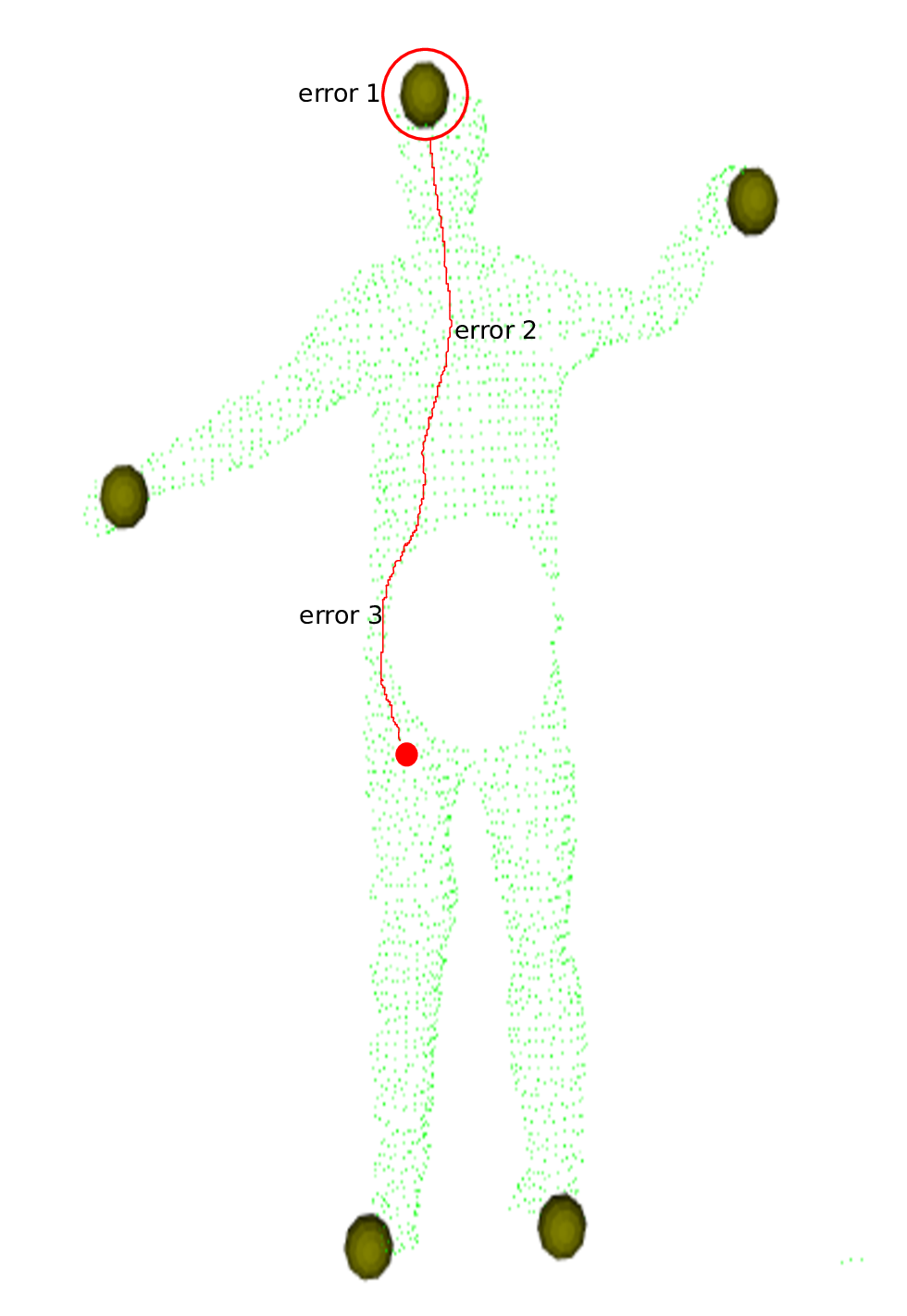
Three errors will reduce the accuracy of feature descriptors based on geodesic distance: (1) errors in localizing the anchors, (2) unmodeled surface mesh deformations, and (3) occlusions, as shown in Figure 4(right). Hence, the measured geodesic distance between and anchor is:
| (12) |
where denotes the true geodesic distance from to , denotes the anchor node localization error, denotes the error due to unmodeled sensor noise, clothes deformations, and underlying musculature, and denotes the geodesic path distortion introduced by the presence of occlusions between and .
The Euclidean distance between the feature vectors of a node and its corresponding node in is:
| (13) |
where , , and . Minimizing these these errors will improve the data association process.
The error captures changes in the geodesic extrema due to noise, and is bounded for bounded sensor noise. Similarly, is bounded since body and cloth distortions between frames are limited in practice. Hence, we can identify a upper limit on , and find all nodes within that limit:
| (14) |
All the nodes in are possible matching vertices of in , if error can be excluded. We choose a node closest to their average position as the most probable match:
| (15) |
This solution is accurate only when the occlusion error can be excluded. We solve this problem with multi-hypothesis tracking: we generate a set of data matching hypothesises and find the one least affected by error term .
IV-D Properties of the Feature Descriptor
For good and robust tracking, a mesh point feature descriptor should be unique and accurate. When all mesh nodes are anchors, uniqueness is guaranteed unless the mesh is highly symmetric. The minimum number of anchor nodes needed to ensure uniqueness is generally unknowable. Our experience shows that, when occlusions are not present, three anchor nodes suffice. Due to the preservation of geodesic distance under deformations, a point feature descriptor will not change during pose changes. If uniqueness holds in one pose, it holds for all poses. Assume that the initial body pose has no self-occlusion, and it is mapped to the Euclidean plane via a bijection. In the Euclidean plane, it is trivial to show that three anchor nodes ensures uniqueness of a point.
The geodesic feature accuracy can degrade under occlusions since geodesic distance to every anchor is not preserved. The preservation of geodesic distance to the anchors depends on the relative anchor locations, and the occlusion size and shape. Next we develop some results on distance preservation with limited convex occlusions. The proofs are eliminated due to length restrictions.
Definition 4
Consider a convex occlusion, , in mesh . For , the bright nodes of are the set of nodes in the boundary of whose geodesic distances to are undistorted. The bright edges of are the edges in the boundary of which connect the bright nodes. The bright region of is the set of bright nodes and edges.
Definition 5
For occlusion in mesh the shadow nodes of are the nodes whose geodesic distance to are distorted by the presence of the occlusion. A shadow edge is an edge in that connects two shadow nodes. The shadowed occlusion boundary are those shadow nodes and edges which lie on the boundary of .
These ideas are illustrated in Figure 5.

Proposition 1
If the bright regions of two nodes, , , on occlusion intersect, then must be undistorted by the presence of .
This result can be extended to the following.
Proposition 2
If the border of occlusion is covered by the union of all anchor point bright regions , then every mesh node will have an undistorted geodesic distance to at least one anchor node.
In the presence of multiple occlusions, some mesh points will experience distorted geodesic distances to all anchoring nodes. A multiple hypothesis testing method, discussed next, helps to alleviate the errors arising in such situations.
V MHT Vertex Tracking
We add a multi-hypothesis-tracing (MHT) framework to further improve data association across frames in the presence of multiple occlusions. MHT requires a gate function, , to generate a set of hypotheses, , which describe the possible correspondences between vertex , and vertices in in : . From the gate function, we construct a tracking tree which links nodes in to their hypothesized children nodes in , where denotes the tree depth. Each branch of is scored, as described below. The scored tree is searched for an optimal association hypothesis.
V-1 Track Tree Construction
We assume that not all geodesic distances between vertices and anchors are corrupted by occlusions. Since we do not know which subset of distances is unaffected, we generate a set of feature descriptor hypotheses for each node , where each hypothesis is based on one possible subset of anchoring nodes.
Based on this idea, we generate a set of possible feature descriptors for vertex :
| (16) |
where denotes the index of each possible subset, denotes the number of anchor nodes in , and denotes one possible subset of nodes.
Each descriptor leads to one hypothetical association of the nodes between two frames, thus for each node , we have possible matched nodes in frame . An example of the possible matches is shown in Figure 6.
Given these hypothesis, we build a track tree by linking nodes to their children in next frame.

V-2 Track Tree Scoring
We score each tree branch to find the best node association hypothesis. Branch is scored on the distance between the measured and predicted node locations
| (17) |
where denotes the tree branch starting from node , and denotes the predicted node locations starting from node . Prediction of the node location in an MHT framework requires a dynamic model to predict movement forward in time.
Because human motion is complex to model, we use a scaled motion dynamics [23] empirical approach to predict node locations. However, any other procedure which provides useful dynamic motion predictions can be used instead.
To construct the scaled motion dynamics model, a reference data set, , of human motions is scaled by interpolation and re-sampling to describe varying speed motion patterns:
| (18) |
where denotes the scaling level, and denotes the number of samples in the reference set. Note that patients undergoing spinal stimulation are asked to carry out highly stereotyped motions, which are well suited to such a modeling approach.
The labeled samples are compared with the training data to find the best matched sub-list:
| (19) |
That is, the current estimate of body motion is used to search the motion data base for similar motions. The most likely motion match is then used to predict the next model state:
| (20) |
Under each hypothesis, a tracked vertex will be occupy a series of locations in subsequent frames. If the hypothesis is not affected by occlusions, these locations will be similar to the dynamic predictions. Otherwise, the hypothesis is likely affected by transient occlusions, and these locations will deviate from the predicted movement patterns.
Then we estimate a set of transformation matrices for all body parts based on the prediction, and then transform each vertex into a predicted location . Repeating this process on the next frames generates a predicted tree for each , which is used to score the tree branches. We restrict rapid tree growth by pruning branches with low scores when the tree size exceeds an empirical threshold.
V-3 Pose Estimation
We search the scored tracking tree for the best hypothetical matching node pairs between frame and , and use these pairs to estimate the joint locations in frame . We construct the global hypothesis by identifying the branch with highest score for each node and extracting the matching node pairs from this branch.
Given the matching node pairs, we use iterative closest points to estimate the transformation matrix for each body part, with the predicted joint locations as initial guess:
| (21) |
The joint locations can be extracted from the updated transformation matrices . One example of the predicted and updated joint locations is shown in Figure 7.

VI Experiments


We test the proposed feature on a data collected with a Kinect V2 sensor. To use scaled motion dynamics to predict the movements, we collect 200 data samples on one subject, with varying movement patterns and speeds that vary from slow, normal to fast. The movement pattern includes upper and lower body movements. For reference the skeletal joint locations estimated by the Kinect sensor on unoccluded data are used as scaled motion dynamics training data. All of the data samples were captured from a front view.
To simulate transient occlusions, we collected 3000 unoccluded data samples of a human body under different types of movements, along with estimated joint locations for ground truth evaluation, and then simulated transient occlusions by removing data from randomly selected frames. We placed occlusions, of five different sizes (radii of 0.03 to 0.15 m), in the center of the body We constructed the surface meshes from the corrupted data via triangulation, and then tried to track the vertices across multiple frames.
The main variables for the geodesic feature are the radius to find the anchor points, the error terms’ upper bounds, and the tracking tree length. We selected a 0.5 m radius empirically, but this parameter can adapt to the subject’s maximum height. An upper bound on the anchors’ localization error was set at a constant 0.05 m. The upper bound on surface point errors was chosen as a linear function increasing with distance, since Kinect error increases with range. The tracking tree look-ahead depth was set to three.
For comparison, we also implemented other local feature-based tracking methods, including fast point feature histogram (FPFH) [8], signature of histograms of orientations (SHOT) [9], 3D shape context (SC) [10], and rotational projection statistics (ROPS) [11]. These local features are invariant under occlusions, and we used them to associate neighboring frames in the tracking framework. We also implemented three local features based on spectral shape analysis: heat kernel signature [16], scale-invariant heat kernel signature [17], and wavelet kernel signature [18].
VI-A Qualitative Results
First, we consider the matching of surface points across frames (under occlusion) with different methods. A descriptor was extracted for each point in successive frames, and points were matched by a nearest neighbor method. Figures 8 and 9 show that the best matching typically occurs in the head, where the surface has stable curvature. Although stable curvatures also exist in the feet and hands, symmetries often cause the swapping of matches. For other body areas, these features generally yield inaccurate matchings due to surface deformations and homogeneous curvatures.
Figure 10 shows the joint locations estimated by our method. While occlusions will cause some mismatches, the method yields adequate estimates of joint locations.
VI-B Quantitative Results


Figures 11 and 12 plot the tracking error and its standard deviation for each occlusion type and joint. The tracking error for each occlusion is the average joint tracking error:
where denotes the estimated joint location under occlusion (ranging from 0 to 0.15 m), and denotes the ground truth. Figure 13 plots the average tracking error for each joint under all types of occlusions: . Figure 14 shows the standard deviation of this error. These results show that our method achieves invariance to transient occlusions like local feature method, while being robust to homogeneous surface regions and deformations. Thus it is more accurate under occlusions.
Besides, it takes about 0.72 seconds to create a mesh with 15549 nodes and 36185 edges on one core of Intel i7-6700 CPU, and about 0.23 seconds to compute the gedoesic feature with five anchor nodes.
VII Conclusions
This work introduced a method to use RGB-D data to track the human body under transient occlusions. The difficulty mainly lies in data association under surface deformations, transient occlusions, and homogeneous surface appearances. Tracking with appearance-based local features are generally robust to transient occlusions, but the tracking is inaccurate due to regions of homogeneous texture, intensity and curvature on human body, and tracking with local features based on spectral shape analysis has similar problems. We propose a solution by designing a geodesic feature robust to surface deformations and homogeneous regions and improving its robustness to transient occlusions by using the multi-hypothesis tracking framework. The result shows that this solution achieves invariance to transient occlusions as well as robustness to homogeneous surface appearances.
Future work will aim to combine the geodesic-feature with appearance-based local features to achieve greater invariance under transient occlusions and greater tracking accuracy.
References
- [1] S. Harkema, Y. Gerasimenko, J. Hodes, J. Burdick, C. Angeli, Y. Chen, C. Ferreira, A. Willhite, E. Rejc, R. G. Grossman et al., “Effect of epidural stimulation of the lumbosacral spinal cord on voluntary movement, standing, and assisted stepping after motor complete paraplegia: a case study,” The Lancet, vol. 377, no. 9781, pp. 1938–1947, 2011.
- [2] S. S. Blackman, “Multiple hypothesis tracking for multiple target tracking,” IEEE Aero. and Elec. Sys. Mag., vol. 19, no. 1, pp. 5–18.
- [3] D. Anguelov, P. Srinivasan, D. Koller, S. Thrun, J. Rodgers, and J. Davis, “Scape: shape completion and animation of people,” in ACM Trans. Graphics, vol. 24, no. 3. ACM, 2005, pp. 408–416.
- [4] M. Dantone, J. Gall, C. Leistner, and L. Van Gool, “Human pose estimation using body parts dependent joint regressors,” in IEEE Conf. Computer Vision and Pattern Recognition, June 2013, pp. 3041–3048.
- [5] J. Shotton, T. Sharp, A. Kipman, A. Fitzgibbon, M. Finocchio, A. Blake, M. Cook, and R. Moore, “Real-time human pose recognition in parts from single depth images,” Commun. ACM, vol. 56, no. 1, pp. 116–124, Jan. 2013.
- [6] A. Agarwal and B. Triggs, “Recovering 3d human pose from monocular images,” IEEE Trans. Pattern Anal. Mach. Intel., vol. 28, no. 1, pp. 44–58, 2006.
- [7] L. Bo and C. Sminchisescu, “Twin gaussian processes for structured prediction,” Int. J. Computer Vision, vol. 87, no. 1-2, pp. 28–52, 2010.
- [8] R. Rusu, N. Blodow, and M. Beetz, “Fast point feature histograms (fpfh) for 3d registration,” in IEEE Int. Conf. Robotics and Automation, May 2009, pp. 3212–3217.
- [9] F. Tombari, S. Salti, and L. Di Stefano, “Unique signatures of histograms for local surface description,” in Computer Vision–ECCV 2010. Springer, 2010, pp. 356–369.
- [10] A. Frome, D. Huber, R. Kolluri, T. Bülow, and J. Malik, “Recognizing objects in range data using regional point descriptors,” in Computer Vision-ECCV 2004. Springer, 2004, pp. 224–237.
- [11] Y. Guo, F. Sohel, M. Bennamoun, M. Lu, and J. Wan, “Rotational projection statistics for 3d local surface description and object recognition,” Int. J. computer vision, vol. 105, no. 1, pp. 63–86, 2013.
- [12] L. Zhang, J. Sturm, D. Cremers, and D. Lee, “Real-time human motion tracking using multiple depth cameras,” in IEEE/RSJ Int. Conf Intell. Robots and Sys., Oct 2012, pp. 2389–2395.
- [13] S. L. Dockstader and A. M. Tekalp, “Multiple camera tracking of interacting and occluded human motion,” Proc. IEEE, vol. 89, no. 10, pp. 1441–1455, 2001.
- [14] A. Zaharescu, E. Boyer, K. Varanasi, and R. Horaud, “Surface feature detection and description with applications to mesh matching,” in IEEE Conf. Comp. Vis. Patt. Rec., June 2009, pp. 373–380.
- [15] T. Darom and Y. Keller, “Scale-invariant features for 3-d mesh models,” IEEE Trans. Image Proc., vol. 21, no. 5, pp. 2758–2769.
- [16] J. Sun, M. Ovsjanikov, and L. Guibas, “A concise and provably informative multi-scale signature based on heat diffusion,” in Computer graphics forum, vol. 28, no. 5, 2009, pp. 1383–1392.
- [17] M. M. Bronstein and I. Kokkinos, “Scale-invariant heat kernel signatures for non-rigid shape recognition,” in IEEE Conf. Comp. Vis. Patt. Rec.. 2010, pp. 1704–1711.
- [18] M. Aubry, U. Schlickewei, and D. Cremers, “The wave kernel signature: A quantum mechanical approach to shape analysis,” in IEEE Int. Conf. Comp. Vis. (Workshops), Nov 2011, pp. 1626–1633.
- [19] A. M. Bronstein, M. M. Bronstein, and R. Kimmel, “Generalized multidimensional scaling: a framework for isometry-invariant partial surface matching,” Proc. Nat. Acad. Sci., vol. 103, no. 5, pp. 1168–72.
- [20] Z. C. Marton, R. B. Rusu, and M. Beetz, “On Fast Surface Reconstruction Methods for Large and Noisy Datasets,” in Proc. IEEE Int. Conf. Robotics and Automation (ICRA), May, 2009.
- [21] R. B. Rusu and S. Cousins, “3D is here: Point Cloud Library (PCL),” in IEEE Int. Conf. Robotics and Automation, Shanghai, May 2011.
- [22] C. Plagemann, V. Ganapathi, D. Koller, and S. Thrun, “Real-time identification and localization of body parts from depth images,” in IEEE Int. Conf. Robotics and Automation, May 2010, pp. 3108–3113.
- [23] B. Rosenhahn and T. Brox, “Scaled motion dynamics for markerless motion capture,” in IEEE Conf. Comp. Vis. Patt. Rec., 2007, pp. 1–8.