The role of coherence in the non-equilibrium thermodynamics of quantum systems

Introduction- The characterization of irreversibility and entropy production has been a central issue of statistical mechanics since the inception of the theory and is by now at the heart of modern approaches to non-equilibrium thermodynamics. For quantum systems [1], fluctuation theorems [2, 3, 4] have been experimentally tested [5, 6] and employed to study irreversibility and to quantify its emergence [7], even in the dynamics of closed systems, driven by external agents that perform work [8, 9, 10] or extract it [11, 12, 13]. Understanding how irreversibility emerges from microscopic laws is not only a fundamental issue [14, 16, 17, 18, 19], it is also a highly pragmatic one. This is particular evident in the current effort to develop thermal machines from small quantum systems [20, 21, 22, 23].

The role played by quantum coherence in thermodynamic settings have been investigated extensively in the past few years [24, 25] but to our knowledge this role lacks a formal clarification. The aim of this letter is to provide precisely this.

Specifically, we will take advantage of the recently introduced measures to quantify coherence [26, 27] and employ the so called relative entropy of coherence to derive quantitative relations between coherence generation and irreversibility. Specifically, we will separate two contributions to the irreversible work produced by a finite time driving, one due to the generation of coherence and a second one due incoherent transitions. Remarkably, we show that the each of the contributions fulfills a fluctuation theorem. Furthermore, we introduce a measure for the non-adiabaticity where the very same coherent contribution can be isolated again, and for which it gives the leading term in slow processes.

We will exclusively focus on generic unitary quantum process, where systems are driven far from an initial equilibrium state $\rho_{0}$ by an external driving described by some suitable Hamiltonian. Here, the system is assumed to be closed, and the time evolution operator $U_{\tau,0}[\lambda]$ is generated by the Hamiltonian $H[\lambda(t)]$, which depends on a work parameter $\lambda(t)$, changed from $\lambda(0)=\lambda_{i}$ to $\lambda(\tau)=\lambda_{f}$ in the time interval $[0,\tau]$. The instantaneous Hamiltonian can be written as $H[\lambda(t)]=\sum_{n}\epsilon_{n}(t)\left|n(t)\right\rangle\left\langle n(t)\right|$, and it changes from $H_{i}\equiv H[\lambda_{i}]$ at $t=0$, into $H_{f}\equiv H[\lambda_{f}]$ at the final time $t=\tau$. Defining the family of free energies $\beta F_{\beta,\lambda}=-\ln Z(\beta,\lambda)$, with the partition function $Z(\beta,\lambda)=\text{Tr}\left\{e^{-\beta H[\lambda]}\right\}$, and the instantaneous equilibrium state, $\rho^{\beta}_{\lambda}=e^{\beta(F_{\beta,\lambda}-H[\lambda])}$, we can write the initial state as $\rho_{0}=\rho^{\beta_{i}}_{\lambda_{i}}$ and its time evolved (out of equilibrium) counterpart as $\rho_{\tau}=U_{\tau,0}[\lambda]\rho_{0}U_{\tau,0}^{\dagger}[\lambda]$. As we are assuming no energy dissipation during the process, the increase in the average energy of the system can be interpreted as work done on it by the driving agent,

where, from now on, every time we write a density matrix element, we understand it is evaluated in the instantaneous energy basis, $\rho_{nm}(t)=\left\langle n(t)\right|\rho_{t}\left|n(t)\right\rangle$. The initial population is, then $\rho_{nn}(0)=\exp\{\beta_{i}(F_{\beta_{i},\lambda_{i}}-\epsilon_{n}(0))\}$, while $\rho_{nn}(\tau)$ can be expressed as $\rho_{nn}(\tau)=\sum_{m}\rho_{mm}(0)P_{m\rightarrow n}(\tau)$ [28], in terms of the transition probability $P_{m\rightarrow n}(\tau)=\left|\left\langle n(\tau)\right|U_{\tau,0}[\lambda]\left|m(0)\right\rangle\right|^{2}$.

Irreversible work and coherence - The energetic deviation between the actual unitary evolution $\rho_{0}\rightarrow\rho_{\tau}$ and the quasi-static isothermal one is known as irreversible work. We would like to stress that the term can be misleading, but in this context we assume that, by definition, the irreversible work is energy which is not recoverable. An isothermal transformation (unlike, e.g., the adiabatic one) is not unitary and would bring the system through a path on the manifold of equilibrium states up to a final state with the same initial inverse temperature $\beta_{i}$, and final Hamiltonian, $\rho_{B}\equiv\rho^{\beta_{i}}_{\lambda_{f}}=\exp\{\beta_{i}(F_{\beta_{i},\lambda_{f}}-H_{f})\}$, see the sketch in Fig. 1. The work performed in this isothermal process is given by the free energy change, $\Delta F=F_{\beta_{i},\lambda_{f}}-F_{\beta_{i},\lambda_{i}}\equiv F_{B}-F_{i}$, and comparing the actual and ideal works, we obtain the so called irreversible work (and entropy),

where the last equality expresses the irreversible entropy as the Kullback-Leibler divergence between the actual final state $\rho_{\tau}$ and the final reference state $\rho_{B}$, $D(\rho_{\tau}||\rho_{B})=-S(\rho_{\tau})-\text{Tr}\left\{\rho_{\tau}\ln\rho_{B}\right\}$, with $S(\rho)$ being the Von Neumann entropy $S(\rho)=-\text{Tr}\left\{\rho\ln\rho\right\}$.

The irreversible work can be decomposed into two contributions, coming from i) unwanted transitions (or, more precisely, from the difference in populations between $\rho_{\tau}$ and $\rho_{B}$), and ii) the coherence generated by the unitary driving during the actual process ($\rho_{B}$, instead, is fully incoherent). Let us first state our first result which we will then prove:

where, the amount of coherence denoted by $C$, is quantified by the relative entropy of coherence of $\rho_{\tau}$ which is defined as

where $I_{\tau}$ is the set of incoherent states in the final energy basis $\{\left|n(\tau)\right\rangle\}$. The second term in Eq. (3), instead, quantifies the population mismatch between the final state $\rho_{\tau}$ and the equilibrium state $\rho_{B}$. This population difference is expressed in terms of the dephasing map in the instantaneous energy basis, $\Delta_{\tau}$, where for $t\in[0,\tau]$,

To prove Eq. (3), we notice that the minimum in Eq. (4) is achieved by $\sigma=\Delta_{\tau}[\rho_{\tau}]$ [27] so that

Since $S(\rho_{\tau})=S(\rho_{0})\equiv S(\Delta_{0}[\rho_{0}])$, the amount of coherence generated in the process, $C(\rho_{\tau})$, coincides with the production of diagonal entropy, as introduced by Polkovnikov [29]. Then,

This equality has a simple physical interpretation: it simply tells us that the amount of irreversible work performed on the system (and, loosely speaking, the amount of irreversibility) can either go into coherence generation, or it can produce non-equilibrium populations (with respect to $\rho_{B}$).

All the steps of the proof above could be repeated for any intermediate time $t\in[0,\tau]$, so that Eq. (3) can be generalized as follows:

where the irreversible work generated up to time $t$ is defined as the average work performed up to $t$ minus the “instantaneous free energy difference”, $\langle w_{irr}(t)\rangle=\text{Tr}\left\{\rho_{t}H[\lambda(t)]\right\}-\text{Tr}\left\{\rho_{0}H_{i}\right\}-(F_{\beta_{i},\lambda(t)}-F_{i})$. Eq. (8) tells us that the decomposition of the irreversible entropy production into a coherent and and incoherent contributions can be performed at any time during the process.

Physical Examples - To gain some insight into this decomposition, we will now focus on studying it in two physically motivated examples. First, we consider the example of a finite time unitary process performed on a qubit. In particular, we focus on the process experimentally realized in Ref. [6], for which we calculated the irreversible work and the fraction of it that is due to coherence generation. The results are reported in Fig. (1).

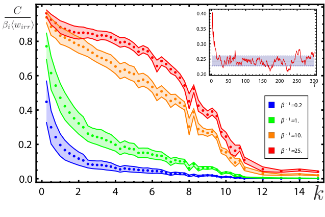
In Fig. 2, we considered the more sophisticated example of a quantum kicked rotor [30], describing a particle freely evolving on a circle, $\hat{H}_{0}=\frac{{\hat{p}}^{2}}{2}$ with $\hat{p}=-i\partial_{\theta}$, and $\theta\in[0,2\pi)$, brought far from its initial equilibrium state by a series of kicks at intervals $T$, $H(t)=H_{0}+V(\theta)\sum_{n\in{\mathds{Z}}}\delta(t-nT)$. In particular, we focus on $V(\theta)=k\cos(\theta)$, leading to the standard quantum map [31]. The state after the $\tau^{th}$ kick will be $\rho_{\tau}=U^{\tau}\rho_{0}{U^{\tau}}^{\dagger}$, with $\hat{U}=e^{-i\hat{H}_{0}T}e^{-iV(\hat{\theta})}$, and with the initial equilibrium state $\rho_{0}=\exp\{-\beta_{i}H_{0}\}/Z_{0}$. Since the Hamiltonian is periodic, the irreversible work coincides with the average work itself, $\langle w_{irr}(\tau)\rangle\equiv\langle w(\tau)\rangle=\text{Tr}\left\{H_{0}(\rho_{\tau}-\rho_{0})\right\}$. The kicks give rise to a spreading of the particle distribution in momentum space. After such a diffusive transient, and due to quantum interference, a relaxation process takes place, giving rise to a localization in momentum space over a width $\xi_{p}$ [33], and (on average over quick fluctuations) to a saturation of the system’s energy. Quantum coherence is essential for such a localization process to occur, and, indeed, $C(\rho_{t})$ is generated during the process. The lower panel of Fig. 2 shows the amount of coherence generated as a function of the kick strength, evaluated in the localized (long time) regime, while the upper panel displays the ratio $C/\langle S_{irr}\rangle$, giving the fraction of irreversible work that is used to produce coherence. More coherence is generated at lower temperatures, but $C$ and $\beta\langle w_{irr}\rangle$ scale differently with $\beta_{i}$ so that the ratio decreases when the temperature is lowered. A simple estimate in terms of the localization parameter gives $\langle w\rangle\sim\xi_{p}^{2}$, while $C\sim\ln(1+\beta\xi_{p}^{2})$, with $\xi_{p}\sim k^{2}$ (for large $k$’s).

Non-adiabaticity - By looking at Fig. (1), one sees that the coherent contribution goes to zero with increasing the process duration $\tau$. This is not an accident, and further insights are gained by studying the energetic deviation from the adiabatic process (rather than from the isothermal one). To this end, we start by recalling the meaning of an ideal quantum adiabatic process. Starting from the same initial equilibrium state $\rho_{0}$, the adiabatic state is $\rho_{A}:=U_{A}\rho_{0}U_{A}^{{\dagger}}$, where $U_{A}$ describes a process in which $\lambda_{i}$ changes into $\lambda_{f}$ with an infinitely slow rate, $U_{A}=\lim_{\tau\rightarrow\infty}U_{\tau,0}[\lambda]$. Under the premises of the quantum adiabatic theorem [34, 35], the system undergoes a transition-less evolution, and $\rho_{A}=\sum_{n}\rho_{A,nn}\left|n(\tau)\right\rangle\left\langle n(\tau)\right|$, with $\rho_{A,nn}=\rho_{nn}(0)$. Generally, this is not a thermal state. However, in Ref. [36], it has been shown that, if this is the case, then one can express the non-adiabatic part of the work, also called inner friction [37], in terms of the non-adiabaticity parameter $\mathcal{A}:=D(\rho_{\tau}||\rho_{A})$, given by the relative entropy between $\rho_{\tau}$ and $\rho_{A}$. This is an operationally useful quantity in itself, which can serve as an entropic quantifier of the deviation from the adiabatic evolution [38]. It can be relevant, e.g., to evaluate the performance of control methods giving rise to shortcuts to adiabaticity [39, 40, 41, 42, 43].

During the actual process, the state of the system is unable to follow the instantaneous adiabatic state, as signaled by a non zero $\mathcal{A}$, due to either the generation of coherence or unwanted diabatic transitions. Indeed, as we did before for the irreversible work, two contributions can be isolated in the non-adiabaticity parameter $\mathcal{A}$ as well, giving

where, again, $C(\rho_{\tau})$ measures the amount of coherence generated by the driving, while $D(\Delta_{\tau}[\rho_{\tau}]||\rho_{A})$ is the contribution to non-adiabaticity given by population changes. The proof of this relation is exactly the same as in Eq. (7), with the only change of $\rho_{A}$ in place of $\rho_{B}$ in every step.

In fact, for slow enough (but yet non-adiabatic) processes, it is the coherence that gives the leading contribution in Eq. (9). To show that this is indeed the case, let us consider a slow enough evolution between $t=0$ and $t=\tau$, so that $U_{\tau,0}[\lambda]$ can be approximated by its adiabatic series expansion in powers of $1/\tau$ [34]. To second order in $\tau^{-1}$, one has

The proof of this approximate relation goes as follows. Up to second order in the adiabatic series, the transition probability is given by [40]

Using this approximation, we can express the diagonal entropy of the actual final state, $S(\Delta[\rho_{\tau}])$, in the form

For the second order transition probabilities, the sum rule $\sum_{n}P^{(2)}_{m\rightarrow n}(\tau)=0$ holds, and therefore

As a result,

which completes the proof of Eq. (9). This relation implies that, as we start to deviate from the adiabatic evolution (that would lead to the incoherent state $\rho_{A}$), the non-adiabaticity parameter $\mathcal{A}$ becomes non-zero due to coherence production, while diabatic transitions give sub-leading contributions.

In the limit $\tau\rightarrow\infty$, $\mathcal{A}$ is zero (by definition), and, thus, $C(\rho_{\tau})$ needs to decay as $\tau$ increases, as in Fig. (1). The fact that $\beta_{i}\langle w_{irr}\rangle$ persists in the long $\tau$ limit, instead, is fully attributable to the second, population term in Eq. (3).

As a final note, for cyclic processes we have $\rho_{A}\equiv\rho_{B}\equiv\rho_{0}$ and therefore the non-adiabaticity parameter coincides with $\langle S_{irr}\rangle$.

Fluctuation relations - In close analogy with the analysis performed by Esposito and Van der Broeck [2], we now show that the separation of the irreversible entropy into a contribution due to coherence generation and another one due to the production of a population mismatch with respect to the reference equilibrium state leads to three integral fluctuation theorems. Adopting the (by now standard) two measurement framework, one imagines to measure energy at $t=0$ obtaining the result $\epsilon_{n}(0)$, and again, at time $t=\tau$, obtaining $\epsilon_{m}(\tau)$ [4]. We can, then, define three stochastic variables that take the values

If these are distributed according to the probability density

then it is a matter of a simple algebra to show that

where the average values are calculated as $\langle\alpha\rangle=\int\alpha P(\alpha)d\alpha$. Indeed, $s$ is just the usual stochastic variable giving irreversible work divided by the initial temperature, $p$ describes the final population mismatch, while $c$ is the difference between the previous two. (Notice that $n$ is a dummy index in $p_{nm}$ and that, accordingly, the summation over $n$ in $P(p)$ is un-effective).

These three variables, whose averages combine as $\langle s\rangle=\langle p\rangle+\langle c\rangle$, satisfy the fluctuation relations

The division of the irreversible entropy production in the two ‘basic’ contributions due to coherence and to population imbalance generation is, thus, in some sense, ‘natural’ in this stochastic framework, as the two parts satisfy independent fluctuation theorems as well. In particular, since $C(\rho_{\tau})$ coincides with the increase in Polkovnikov’s diagonal entropy, the relation $\langle e^{-c}\rangle=1$ provides a fluctuation theorem for it which is quite remarkable and suggests an interesting, uniquely quantum aspect to certain transformations in non equilibrium thermodynamics.

Conclusions - Let us summarize our results. We have shown, using the concept of relative entropy of coherence, that a uniquely coherent contribution to the energetics of a driven quantum system can be identified. Given the current interest and development of thermodynamics of non equilibrium quantum systems, this is an important result and can be used to analyze in detail the role of coherence in thermodynamic transformations. We have illustrated our result with two physical examples. Furthermore, we have shown that this coherence term appears also in the quantification of non-adiabaticity and that, up to second order in the adiabatic expansion, the coherence is actually a measure of the deviation from adiabatic evolution. Furthermore, in this framework, coherence generation coincides with the increase in diagonal entropy, and, thus, our analysis clarifies the role of the latter in quantum thermodynamics. Finally we have shown that the coherence itself obeys a fluctuation theorem.

References

- [1] M Campisi, P Hänggi, Entropy 13, 2024 (2011); J. Goold, M. Huber, A. Riera, L del Rio, and P. Skrzypczyk, J. Phys. A: Math. Theor. 49, 143001 (2016); R. Kosloff, Entropy 15, 2100 (2013); S. Vinjanampathy, and J. Anders, Contemp. Phys. 57, 1 (2016); D. Gelbwaser-Klimovsky, W. Niedenzu, and G. Kurizki, Adv. Atom. Mol. Opt. Phys. 64, 329 (2015); S. Wehner, M. M. Wilde, M. P. Woods, arXiv:1506.08145 (2015).
- [2] C. Jarzynski, Phys. Rev. Lett. 78, 2690 (1997); G. E. Crooks, Phys. Rev. E 60, 2721 (1999); H. Tasaki, arXiv:cond-mat/0009244 (2000); J. Kurchan, arXiv:cond-mat/0007360 (2001); S. Mukamel, Phys. Rev. Lett. 90, 170604 (2003); M. Esposito, and C. Van den Broeck, Phys. Rev. Lett. 104, 090601 (2010).
- [3] M. Esposito, U. Harbola, and S. Mukamel, Rev. Mod. Phys. 81, 1665 (2009); C. Jarzynski, Annu. Rev. Condens. Matter Phys. 2 329 (2011); U. Seifert, Rep. Prog. Phys. 75, 126001 (2012); P. Hänggi and P. Talkner, Nat. Phys. 11, 108 (2015).
- [4] M. Campisi, P. Ha̋nggi, and P. Talkner, Rev. Mod. Phys. 83, 771 (2011).
- [5] T. B. Batalhão, A. M. Souza, L. Mazzola, R. Auccaise, R. S. Sarthour, I. S. Oliveira, J. Goold, G. De Chiara, M. Paternostro, and R. M. Serra, Phys. Rev. Lett. 113, 140601 (2014); S. An, J.-N. Zhang, M. Um, D. Lv, Y. Lu, J. Zhang, Z.-Q. Yin, H. T. Quan, and K. Kim, Nat. Phys. 11, 193 (2015).
- [6] T. B. Batalhão, A. M. Souza, R. S. Sarthour, I. S. Oliveira, M. Paternostro, E. Lutz,5 and R. M. Serra, Phys. Rev. Lett. 115, 190601 (2015).
- [7] S. Deffner and E. Lutz, Phys. Rev. Lett. 105, 170402 (2010); S. Deffner, E. Lutz, Phys. Rev. Lett. 107, 140404 (2011).
- [8] P. Talkner, E. Lutz, and P. Hänggi, Phys. Rev. E 75, 050102(R) (2007).
- [9] R. Dorner, S. R. Clark, L. Heaney, R. Fazio, J. Goold, and V. Vedral, Phys. Rev. Lett. 110, 230601 (2013); L. Mazzola, G. De Chiara, and M. Paternostro, Phys. Rev. Lett. 110, 230602 (2013);
- [10] G. De Chiara, A. J. Roncaglia, and J. P. Paz, New J. Phys. 17, 035004 (2015).
- [11] J. Åberg, Nat. Commun. 4, 1925 (2013); P. Skrzypczyk, A. J. Short, S. Popescu, Nat. Comm. 5, 4185 (2014).
- [12] A. E. Allahverdyan, R. Balian and Th. M. Nieuwenhuizen, Europhys. Lett. 67, 4 (2004).
- [13] G. Francica, J. Goold, F. Plastina, M. Paternostro, npj Quantum Information 3, 12 (2017).
- [14] T. D. Kieu, Phys. Rev. Lett. 93, 140403 (2004).
- [15] M. Esposito, C. Van den Broeck, Europhys. Lett. 95, 40004 (2011).
- [16] H. Tasaki, Phys. Rev. Lett. 116, 170402 (2016).
- [17] U. Seifert, Phys. Rev. Lett. 116, 020601 (2016).
- [18] V. Cavina, A. Mari, and V. Giovannetti, Sci. Rep. 6, 29282 (2016).
- [19] F. Brandão, M. Horodecki,N. Ng, J. Oppenheim, S. Wehner, Proceedings of the National Academy of Sciences 112, 3275 (2015).
- [20] O. Abah, J. Roßnagel, G. Jacob, S. Deffner, F. Schmidt-Kaler, K. Singer, E. Lutz, Phys. Rev. Lett. 109 203006 (2014); J. Roßnagel, O. Abah, F. Schmidt-Kaler, K. Singer, E. Lutz, Phys. Rev. Lett. 112 030602 (2014).
- [21] J. Roßnagel, S. T. Dawkins, K. N. Tolazzi, O. Abah, E. Lutz, F. Schmidt-Kaler, and K. Singer, Science 352, 6283 (2016); A. Dechant, N. Kiesel, and E. Lutz, Phys. Rev. Lett. 114, 183602 (2015).
- [22] J. P. Pekola, P. Solinas, A. Shnirman, D. V. Averin, New J. Phys. 15, 115006 (2013); M. Campisi, J. Pekola, and R. Fazio, New J. Phys. 17, 035012 (2015).
- [23] M. Campisi, R. Fazio, Nat. Commun. 7, 11895 (2016).
- [24] M. Scully, M. S. Zubairy, G. S. Agarwal, and H. Walther, Science 299, 862 (2003); M. Scully, Phys. Rev. Lett. 104, 207701 (2010).
- [25] J. Åberg, Phys. Rev. Lett. 113, 150402 (2014); N. H. Y. Ng, L. Mančinska, C. Cirstoiu, J. Eisert, S. Wehner, New. J. Phys, 17, 085004 (2015); M. Lostaglio, D. Jennings, and T. Rudolph, Nat. Commun. 6, 6383 (2015); M. Lostaglio, K. Korzekwa, D. Jennings, and T. Rudolph, Phys. Rev. X, 5, 021001 (2015); P. Kammerlander, J. Anders, Sc. Rep. 6, 2174 (2016).
- [26] T. Baumgratz, M. Cramer, and M.B. Plenio, Phys. Rev. Lett. 113, 140401 (2014).
- [27] A. Streltsov, G. Adesso, and M. B. Plenio, arXiv:1609.02439v1 (2016)
- [28] A. Polkovnikov, Phys. Rev. Lett. 101, 220402 (2008).
- [29] A. Polkovnikov, Ann. Phys. 326, 486 (2011).
- [30] G. Casati et al., Lect. Notes Phys. 93, 334 (1979).
- [31] F. M. Izrailev, Phys. Rep. 196, 299 (1990).
- [32] B. Sundaram and G. M. Zaslavsky, Phys. Rev. E 59, 7231 (1999).
- [33] S. Fishman, D. R. Grempel and R. E. Prange, Chaos, Phys. Rev. Lett. 49, 509 (1982).
- [34] A. Messiah, Quantum Mechanics, North Holland, Amsterdam (1970).
- [35] A. E. Allahverdyan, Th. M. Nieuwenhuizen, Phys. Rev. E 71, 046107 (2005).
- [36] F. Plastina, A. Alecce, T.J.G. Apollaro, G. Falcone, G. Francica, F. Galve, N. Lo Gullo, and R. Zambrini, Phys. Rev. Lett. 113, 260601 (2014).
- [37] R. Kosloff, and T. Feldmann, Phys. Rev. E 65, 055102 (2002); R. Kosloff, and T. Feldmann, Phys. Rev. E 68, 016101 (2003); R. Wang, J. Wang, J. He, and Y. Ma, Phys. Rev. E 87, 042119 (2013); A. Alecce, F. Galve, N. Lo Gullo, L. dell’Anna, F. Plastina, R. Zambrini, New J. Phys. 17, 075007 (2015).
- [38] G. Francica et al., in preparation.
- [39] E. Torrontegui, S. Ibáñez, S. Martínez-Garaot, M. Modugno, A. del Campo, D. Guéry-Odelin, A. Ruschhaupt, X. Chen, and J. G. Muga, Adv. At. Mol. Opt. Phys. 62, 117 (2013).
- [40] M. V. Berry, J. M. Robbins, Proc. R. Soc. London, Ser. A, 442, 659 (1993).
- [41] X. Chen, A. Ruschhaupt, S. Schmidt, A. del Campo, D. Guéry-Odelin, and J. G. Muga, Phys. Rev. Lett. 104, 063002 (2010); J.-F. Schaff, X.-L. Song, P. Vignolo, and G. Labeyrie, Phys. Rev. A 82, 033430 (2010); J.-F. Schaff, X.-L. Song, P. Capuzzi, P. Vignolo, and G. Labeyrie, Europhys. Lett. 93, 23001 (2011); M. G. Bason, M. Viteau, N. Malossi, P. Huillery, E. Arimondo, D. Ciampini, R. Fazio, V. Giovannetti, R. Mannella, and O. Morsch, Nat. Phys. 8, 147 (2012); J. W. Deng, Q.-H. Wang, Z. H. Liu, P. Hänggi, and J. B. Gong, Phys. Rev. E 88, 062122 (2013); M. Palmero, E. Torrontegui, D. Guéry-Odelin, and J. G. Muga, Phys. Rev. A 88, 053423 (2013).
- [42] A. del Campo, M. M. Rams, and W. H. Zurek, Phys. Rev. Lett. 109, 115703 (2012); A. del Campo, Phys. Rev. Lett. 111, 100502 (2013); S. Deffner, C. Jarzynski, and A. del Campo, Phys. Rev. X 4, 021013 (2014); A. del Campo, J. Goold, and M. Paternostro, Sci. Rep. 4, 6208 (2014); T. V. Acconcia, M. V. S. Bonança, and S. Deffner, Phys. Rev. E 92, 042148 (2015).
- [43] Y. Zheng, S. Campbell, G. De Chiara, and D. Poletti, Phys. Rev. A 94, 042132 (2016)