Constraining interacting dark energy with CMB and BAO future surveys
Abstract
In this paper, we perform a forecast analysis to test the capacity of future baryon acoustic oscillation (BAO) and cosmic microwave background (CMB) experiments to constrain phenomenological interacting dark energy models using the Fisher matrix formalism. We consider a Euclid-like experiment, in which BAO measurements is one of the main goals, to constrain the cosmological parameters of alternative cosmological models. Moreover, additional experimental probes can more efficiently provide information on the parameters forecast, justifying also the inclusion in the analysis of a future ground-based CMB experiment mainly designed to measure the polarization signal with high precision. In the interacting dark energy scenario, a coupling between dark matter and dark energy modifies the conservation equations such that the fluid equations for both constituents are conserved as the total energy density of the dark sector. In this context, we consider three phenomenological models which have been deeply investigated in literature over the past years. We find that the combination of both CMB and BAO information can break degeneracies among the dark sector parameters for all three models, although to different extents. We found powerful constraints on, for example, the coupling constant when comparing it with present limits for two of the models, and their future statistical 3- bounds could potentially exclude the null interaction for the combination of probes that is considered. However, for one of the models, the constraint on the coupling parameter does not improve the present result (achieved using a large combination of surveys), and a larger combination of probes appears to be necessary to eventually claim whether or not interaction is favored in that context.
I Introduction
Cosmic microwave background (CMB) measurements have contributed to an unprecedented understanding of the universe at its early stages, leading us to a well-established and consistent picture of how the universe is today. Recent results from the Planck satellite collaboration showed that baryonic matter constitutes about of all that is known, leaving about of ‘dark’ components [1, 2]. The cold dark matter (CDM) accounts for roughly of the universe, and the remaining is in the form of dark energy (DE). Considering the standard cosmological model, the DE assumes its simplest form as a cosmological constant , leading to the so-called CDM model. Based on general relativity, the cosmological constant viewed as a DE fluid with equation of state (EoS) , where is the pressure and the energy density, can explain well the current accelerated expansion of the universe [3, 4].
Despite of successfully explaining the observations, the CDM model faces some difficulties [5], especially in the dark sector. Dark matter (DM) particles have not been detected yet, and their origin, presumably beyond the standard model of particles physics, is still unknown (see, e.g., Ref. [6] and references therein). Theoretical calculations of the vacuum energy density estimate the value of the cosmological constant to be orders of magnitude larger than its actual observed value (see, e.g., Ref. [7]). In addition, the present values of the DM and DE densities are of the same order of magnitude even though they do not share the same cosmological evolutionary behaviour. This cosmic coincidence seems to indicate that we are living in a special epoch of the cosmic history [8]. To overcome some of these problems, researchers started to consider models in which DM and DE interact, and these became very useful in alleviating this coincidence problem (see, e.g., Refs. [9, 10, 11, 12, 13, 14, 15, 16]). An interacting DM and DE scenario would affect the overall evolution of the universe and its expansion history, thus it is observationally distinguishable from the CDM model. The interaction can then be constrained by the data, becoming a testable theory for the universe.
Present observations, however, are not able to confidently distinguish between these alternative interacting DE models and CDM. Updated cosmological data have already been confronted with such models (see, for example, Refs. [15, 16, 18, 17, 19, 20, 21, 22, 23, 24, 25, 26, 27]), but often a null interaction cannot be discarded with high confidence. Nevertheless, Ref. [28] claims that interacting models can explain the high-redshift observations of the Baryon Oscillation Spectroscopic Survey (BOSS) [29], which deviate from CDM. In this context, future generation of astronomical ground- and space-based experiments as well as future CMB experiments will be able to precisely perform consistency tests of the CDM model and significantly improve constraints on alternative scenarios, including the interacting DE models. A lot of effort has been made to constrain and forecast parameters in alternative DE scenarios in the past years (see, for instance, Refs. [30, 31, 32, 33]). However, for interacting DE models, only recently, Ref. [34] performed a forecast analysis of the capability of eLISA to constraint such models, finding that it can only be competitive if the onset of the deviation from CDM of these models occurs relatively late in the evolutionary history of the universe. Earlier studies are outdated since they have explored the forecast of Planck-like CMB surveys alone on phenomenological interacting DE models [35] or with earlier configurations of Euclid-like experiments [36]. Others have explored the forecast for field theory implementations of coupled DE [37]. In this paper, we consider a combination of future state-of-the-art probes: the baryon acoustic oscillations (BAO) information that can be obtained from an updated Euclid-like experiment [38] and the primary CMB fluctuations from a possible future experiment like AdvACT [39]. The goal is to test their ability to constrain the phenomenological interacting DE models described in this paper and determine how their combination can help break the degeneracies between the different cosmological parameters.
The paper is organized as follows. In Sec. II, we describe the phenomenological models with which we perform the parameter forecast. Sec. III is devoted to the methodology we use to calculate the marginalized errors on the chosen parameters, followed by the results in Sec. IV. Finally, in Sec. V, we draw our conclusions.
II The interacting dark energy models
In the standard cosmological model, the energy momentum tensor for radiation, baryons, cold DM, and DE is conserved separately, i.e., for each component. Conversely, in an interacting DE model, the fluid equations for the DE and DM are not conserved individually, but the dark sector as a whole satisfies the usual energy-conservation equation. In a Friedmann-Robertson-Walker universe, the conservation equations for the fluids that exchange energy are:
| (1) |
where is the Hubble parameter, and are the energy densities for DM and DE, respectively, and is the DE EoS. It is clear from the DM conservation equation that we assume , i.e., the DM EoS is that of pressureless matter (dust). Here, represents the interaction kernel that can be written phenomenologically as , where the coupling coefficients (the constants and ) are to be determined by observations (see, e.g., Refs. [14, 15, 28, 17, 16, 40, 41]). The energy flow from DE to DM is defined by , and conversely, defines an energy flow from DM to DE. Considering the stability of the cosmological perturbations when is kept constant, two choices can be made [42]: first, one can take and , together with a constant DE EoS within the range (dubbed model 1) or (model 2); second, one can take and with , defining our third considered model (for a summary, see Table 1). For all three models, the other components follow the standard conservation equations. For a review of the topic, we refer to Refs. [43, 16].
| Model | DE EoS | |
|---|---|---|
| 1 | ||
| 2 | ||
| 3 |
When one allows for an energy flow between DE and DM, the energy densities present a different evolution for each model. The presence of this change in the redshift dependency leads to an effective EoS for DM and for DE, which depends on the form of the interaction. For models 1 and 2, the energy densities for DM and DE are given by (see Ref. [41])
| (2) |
and the effective equations of state are
| (3) |
with . For model 3, the evolution of the energy densities follows
| (4) |
and the effective equations of state are
| (5) |
In both cases, the baryon energy density () is given by the standard expression, i.e., it is proportional to . Note that the quantities measured today are identified by the superscript . For example, using the definition of the cold DM density parameter today, , where is the critical density of the universe, one has
| (6) |
where we use the same notation as in Ref. [1] with defined such that , and where and are the Hubble parameter and the physical density of cold DM today.
Since DM and DE are currently only measured gravitationally and since gravity only probes the total energy momentum tensor, degeneracies in the cosmological parameters are inevitable. As it is already known in the literature (see, e.g., Refs. [44, 14, 45]), and as we can see in the expressions for the energy densities of the coupled dark components, there is a degeneracy between and . At the background level, the fact that only the total energy momentum can be measured also leads to a degeneracy between the coupling constant and , as we can see in the effective DE EoS for models 1 and 2 [see Eq. (3)]. For model 3, this degeneracy is no longer present today since for (i.e., when ). In that case, the DE EoS and the interacting constant can be measured independently using the background evolution [14].
To be able to compare theoretical predictions from the different phenomenological models with experiments, the cosmological perturbations for these models have been calculated in Ref. [14]. In this reference, the linear perturbations are calculated by perturbing the Friedmann-Lemaître-Robertson-Walker spacetime and the energy-momentum tensor of the coupled DM-DE fluid. First, the background interaction four-vector is given by , which represents the exchange of energy density only [c.f. Eq. (1)]. The subscript stands for either DE in the case of models 1 and 2 or DM in the case of model 3. Then, the perturbed four-vector representing the perturbation in the interaction between the DM and DE fluids, , can be decomposed into
| (7) |
The sign refers to DM or DE respectively; is the potential of the perturbed energy-momentum transfer ; is the external non-gravitational force density; and is the average velocity of the energy transfer. Since we have a stationary energy transfer, we only consider inertial drag effects, so and vanish, which implies that . One can then evaluate the linear order perturbation equations for DM and DE (we refer to Ref. [14] for more details; see also Ref. [46] for another study of the perturbations in this context).
With the perturbations, one can then compute the CMB temperature angular power spectrum () and the matter power spectrum (). The corresponding spectra are shown for different values of the coupling constant for each of the models described in Table 1 in Figs. 1 (model 1), 2 (model 2), and 3 (model 3). By computing the perturbations, one can also evaluate the growth rate () and the root mean square of matter fluctuations today at a characteristic length scale of () in order to illustrate how the interaction affects the growth of structure. This is shown in Fig. 4. The plots are generated using a modified version of the CAMB software package [47], which incorporates the physics of interacting DE. Moreover, the cosmological parameters (excluding the values for the coupling constants and for the power spectra) are assumed to take the fiducial values given in Sec. III, see Table 3 for Fig. 1, Table 4 for Fig. 2, and Table 5 for Fig. 3.
As noted in Ref. [14], changes in the DE EoS mainly influence the low- angular power spectrum and can shift the overall amplitude of the matter power spectrum slightly. For this reason, we only show the changes caused by varying the coupling constant in the power spectra. From the plots, we see that interacting DE can have effects that are degenerate with changing the DE EoS, but these degeneracies can be broken by including all the information from both the CMB angular power spectrum and the matter power spectrum today. Indeed, interacting DE generally changes the size of the CMB acoustic peaks and it affect the amplitude of only at large , which can hardly be mimicked by a different EoS.
Generally, we can see that for large couplings (), the changes in the acoustic peaks of the power spectra compared to CDM () are very pronounced, so large couplings can be easily ruled out by observations. However, in general, small couplings introduce more subtle changes that are harder to be distinguished, and from previous analyzes, small couplings are preferred by the observations [15, 16, 17, 18, 19, 20, 21, 22, 23, 24, 25, 26, 27, 28], although with small significance. Although subtle, these changes behave differently depending on the model chosen, so it is important to understand how each model affects the power spectra.
For model 1, let us first note that the interacting constant must be negative [17]. This means that there is an energy flow from DM to DE and that the DM energy density is higher in the past compared to CDM. As we can see in Fig. 1, having more DM in the past leads to an overall suppression of the angular power spectrum together with a small change in the low- behaviour. This extra amount of DM influences the evolution of matter perturbations, leading to more structure formation, as it can be seen in Fig. 4. The growth rate is always higher than in CDM, especially at low redshifts when DE starts to dominate at which point these effects become more pronounced. This also affects at low-redshifts. As a result, there is an enhancement in the amplitude of the matter power spectrum, mainly on scales smaller than the turn-around point due to the fact that the matter-radiation equality happened earlier in the evolution of the universe, thus decreasing the amount of damping of the small-scale modes during radiation domination.
For models 2 and 3 (see Figs. 2 and 3), one has a positive coupling constant, meaning that there is less DM in the past in comparison with CDM, as DE gets converted into DM as time evolves. This leads to an enhancement of the overall amplitude of the peaks in the angular power spectrum caused by shallower DM gravitational potentials, leading to the elimination of baryon loading. This affects the evolution of the matter perturbations, which can be seen by a slightly smaller growth rate, for model 2 (see Fig. 4). This change is very subtle for model 3, since the density of DM does not depend so strongly on the energy density of DE, but its deviation from the standard dust behaviour depends mainly on the interaction [14]. The effect on the matter power spectrum is a change in the turn-around position, caused by the matter-radiation equality being shifted to lower redshifts in comparison to CDM, which in turn leads to damping on small scales. Model 3 presents a more pronounced effect for a large coupling, as we can see in Fig. 3. This choice of large coupling is not realistic and excluded by observations, but it serves to illustrate the effects that the interaction has in the power spectrum and the possible degeneracy between the coupling and .
As we saw above, changes in the power spectra from the interaction between DM and DE can be mimicked by changing or by a different EoS of DE, showing again the degeneracy between the coupling constant, , and the EoS of DE. In order to measure a small coupling between DM and DE and to improve the constraints on the cosmological parameters, we need future generations of cosmological observations and complementary observations that can break the degeneracy between the interacting DE parameters and the DM energy density. Different observations probe DE and other cosmological parameters in different ways. For this reason, in what follows, we explore the combination of CMB and BAO observations as a mean to break degeneracies. We will show that some of those degeneracies can indeed be broken by combining CMB and BAO measurements, but to fully break the degeneracies, growth of structure measurements like weak lensing and galaxy clustering (that would measure, e.g., as shown in Fig. 4) should be included. We keep this for follow-up work. For a first theoretical analysis of the growth of structures in interacting DE models, see Refs. [48, 25].
III Methodology
III.1 Information from galaxy surveys: baryon acoustic oscillation
The baryon acoustic oscillation (BAO) is an important observable currently used to constrain the cosmological parameters more efficiently in combination with other probes such as the CMB. The information stored in the BAO peaks present in the matter power spectrum can be used to determine the Hubble parameter and the angular diameter distance as a function of the redshift, which subsequently allows us to calculate the DE parameters. Let us first define the observed power spectrum in redshift space using a particular reference cosmology (in our case, CDM), which differs from the true cosmology (for details about this methodology, see Ref. [49]), as follows,
| (8) |
where is the unknown Poisson shot noise. The Hubble parameter and angular diameter distance values in the reference cosmology (CDM) are distinguished from the values in the true cosmology by the superscript ‘(ref)’.
The angular diameter distance is given by
| (9) |
hence it depends on the evolution of the Hubble parameter. We can write as a function of the DE and DM parameters, knowing that it is related to the DE and DM densities through the Friedmann equation,
| (10) |
where the evolution of the different energy densities depend on the model chosen as seen in Sec. II [cf. Eqs. (2) and (4)].
The wavenumbers across and along the line of sight in the true cosmology are denoted by and , and they are related to the ones in the reference cosmology by and . The galaxy power spectrum, , can be written as follows:
| (11) |
In the equation above, we defined , where is the unit vector along the line of sight. The exponential damping factor is due to redshift uncertainties (), where . Also, , , and are the growth function, the linear redshift space distortion parameter, and the linear galaxy bias, respectively, which are related through the definition . The linear matter power spectrum, , as well as the growth rate, , are generated using a modified version of CAMB to account for the physics of interacting DE. The effect of the interaction in these models was described in the previous section.
The above provides the necessary information to perform a Fisher matrix forecast for future BAO experiments. The Fisher matrix formalism has become the standard method for predicting the precision with which various cosmological parameters can be extracted from future data. The advantage of it relies on the fact that it is a fast approach and generally returns accurate estimates for the parameter errors from the derivatives of the observables with respect to the model parameters around the best fit value. We note, though, that it is not always justified to use the Fisher matrix approach as opposed to a Monte Carlo Markov Chain (MCMC) posterior likelihood estimation method (see, e.g., Ref. [50]). This is especially true when one does not know whether the cosmological parameters of the given theoretical model will be Gaussian or not for a given set of cosmological data. This is why older studies have preferred an MCMC approach [35, 36], but these papers have shown that the estimated likelihood contours for cosmological parameters of phenomenological interacting DE could be well-approximated by Gaussian ellipses. Furthermore, many MCMC analyzes with current data have shown similar Gaussian-like likelihood curves. Hence, we believe that the Fisher matrix approach is well justified in this case, though we must keep in mind that the constraints found are probably lower bounds on the marginalized errors (i.e., it is the best-case scenario).
For the matter power spectrum obtained from galaxy surveys, the Fisher matrix is given by (see Ref. [51])
| (12) |
where and are elements of the set of parameters for the given cosmological model. The effective volume of the survey, , can be written, for a constant comoving number density (), as
| (13) |
In this paper, we present the expected cosmological implications of the BAO measurements for a Euclid-like survey (for specifications of the Euclid survey, see, for example, Ref. [38] and references therein). We assume an area of , a redshift accuracy of , and a redshift range .
We then take 15 redshift bins of width centered on . The set of parameters of interest to obtain constraints on the dark sector is . For a given redshift slice, the parameters , , , , and are estimated simultaneously with , , and and according to the assumed fiducial values of a set of cosmological parameters for each considered model. The total number of parameters is for a BAO survey divided in redshift bins. The derivatives of the observable with respect to the model parameters in Eq. (12) are then evaluated at the fiducial values, which we take to be the best-fit values of Ref. [17] for each considered interacting DE model. Finally, we must derive the errors on and to later propagate them into the desired dark sector parameters for the interacting DE models.
After marginalizing the Fisher matrix defined above over , , and , a sub-matrix is then calculated as follows,
| (14) |
where and , the latter being the final set of parameters defined as for models 1 and 2 and for model 3.
The constraints on the dark sector parameters are then determined by how well the survey is able to estimate the values of and .
III.2 Information from CMB
In the context of cosmological parameters forecast, we use the CMB information as a second probe to test the ability of future surveys to constrain a possible interaction in the dark sector and possibly to distinguish between the different interacting models described previously and the CDM model. We use the modified CAMB software package [47] to generate the numerical power spectra () for our cosmological models with . We do not consider primordial -modes (i.e., we assume a vanishing primordial tensor power spectrum) or CMB lensing in the analysis. The latter is justified by the fact that the HALOFIT [52] non-linear implementation present in CAMB has only been tested against N-body simulations for CDM cosmologies and the non-linear structure evolution starts to affect the lensing signal already at (see Ref. [53] for studies of CMB lensing and of the non-linear regime in coupled DE cosmologies). We then construct the Fisher matrix for the CMB temperature anisotropy and polarization as follows (see Ref. [54]),
| (15) |
where represents the power in the -th multipole, and where stands for (temperature), (-mode polarization), and (temperature and -mode polarization cross-correlation). The covariance matrix is given by
| (16) |
and the elements of the matrix are given in Appendix A.
| Frequency [GHz] | - | |
|---|---|---|
| 90 | 7.8 | |
| 150 | 6.9 | |
| 230 | 25 |
In the near future, CMB surveys will continue to improve, especially ground-based instruments designed to measure polarization. The Advanced Atacama Cosmology telescope (AdvACT) [39] is expected to obtain precise measurements of the CMB small-scale polarization, enabling us to tackle a wide range of cosmological physics. In particular, it will tighten the constraints on the cosmological parameters of alternative models to CDM. The instrumental setup of AdvACT is outlined in Table 2. This is the information that we incorporate in our Fisher matrix analysis to obtain the CMB forecast (see Appendix A for details about how noise is handled).
IV Results and discussion
Following the methodology described in the previous section, we compute the Fisher matrices for the three interacting DE models presented in Sec. II considering a Euclid-like future BAO survey and an AdvACT-like future CMB experiment. We also consider the combination of BAO and CMB future measurements. Assuming that the probes are uncorrelated, one can add the Fisher matrices as follows [55]
| (17) |
| Parameter | Fiducial | AdvACT | Euclid | AdvACT + Euclid |
|---|---|---|---|---|
| value | (CMB) | (BAO) | ||
| 0.02224 | 3.86e-05 | 0.00028 | 3.69e-05 | |
| 0.08725 | 0.017 | 0.0017 | 0.00053 | |
| 0.6845 | 0.0079 | 0.0055 | 0.0014 | |
| -0.9434 | 0.028 | 0.026 | 0.0044 | |
| -0.0929 | 0.045 | 0.0037 | 0.0019 |
We first show the result for model 1 in Table 3, where the different columns represent the cosmological parameter, its fiducial value, and the 68% confidence level (C. L.) constraints that would result from AdvACT, Euclid, and the combination of AdvACT and Euclid, respectively. We notice that the marginalized error for the DE EoS improves drastically for the combined analysis, being for Euclid, for AdvACT, and for their combination: an improvement by a factor of when compared with each individual probe. The constraint on the DM density improves by a factor of for the combined analysis (), compared with Euclid alone (). A similar improvement occurs for the coupling constant, where we find for Euclid alone and for . Such a stringent constraint would exclude the null interaction corresponding to CDM with high confidence given that the contours from global fits would be centered on values close to the fiducial values used in this analysis.
Present constraints on , , and for a combination of probes (Planck+BAO+SNIa+H0; see Ref. [17]) are found to be , , and . The fact that our forecast suggests that future surveys will greatly improve these constraints can be seen from the confidence regions of cosmological parameters related to the dark sector. In Fig. 5, we plot the marginalized confidence ellipses at 1 and 3 for the combinations of , , and for AdvACT (red), Euclid (blue), and (green) for model 1. The constraints on the cosmological parameters are affected by the degeneracies present among them. In order to assess these degeneracies and to see how introducing new observations like BAO from Euclid can affect them, we introduce the correlation matrix , which measures the correlation between two parameters and . It is given by
| (18) |
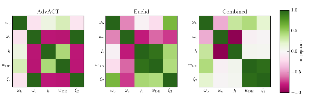
where , and is either the CMB, BAO, or total Fisher matrix. The correlation coefficient for ranges from 0 (the two parameters are completely independent) to (the parameters are completely (anti-)correlated). The correlation matrix is depicted in Fig. 6 for model 1 where white, dark magenta, and dark green are equivalent to , , and , respectively.
| Parameter | Fiducial | AdvACT | Euclid | AdvACT + Euclid |
|---|---|---|---|---|
| value | (CMB) | (BAO) | ||
| 0.02229 | 3.85e-05 | 0.00022 | 3.76e-05 | |
| 0.1314 | 0.015 | 0.0030 | 0.0010 | |
| 0.6876 | 0.075 | 0.0068 | 0.0019 | |
| -1.087 | 0.19 | 0.033 | 0.0053 | |
| 0.03798 | 0.055 | 0.0055 | 0.0031 |
For model 1, when only CMB information is provided, the dark sector parameters and are very (anti-)correlated as pointed in Sec. II, which can be seen by visual inspection of Fig. 5. We can see that the correlation between and is (in absolute value) and it is very large () between and as well (see Fig. 6). These degeneracies are considerably weakened when BAO information is added. For instance, the correlations between and and between and are reduced to and , respectively, for the combined forecast (). The correlation between and changes sign in comparison with CMB alone, and the level of degeneracy between these parameters is only mildly alleviated. This happens since the degeneracy is present between the three parameters , and , and BAO only helps constraining one of them, leaving some degeneracy among the other two (or combinations of such parameters). In summary, these results show that BAO has the power to break some degeneracies, as we can see by the tighter constraints and the milder correlations encountered, although there remains some degeneracies among parameters.
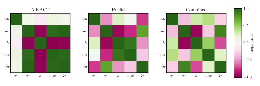
Similar results are found for model 2 as it can be seen in Table 4 and Figs. 7 and 8. The combined forecast leads to stringent constraints on , , and , the latter being . It was claimed by Ref. [18] that an energy flow from DE to DM (), resulting in a non-zero coupling between the two dark components where DE decays into DM, is in better agreement with present cosmological data. A vanishing interaction is also excluded by Ref. [17] with (the errors are given at 68% C. L.). The future combination of AdvACT and Euclid-like surveys would be able to improve this constraint by a factor of , hence one could potentially distinguish the interacting DE model from CDM (and equivalently from CDM) by more than 3 (and possibly even more than 5). Of course, a proper statistical analysis would have to be done in order to really assess which model is preferred by the data. From the correlation matrix (Fig. 8), we can see, like in the previous case for model 1, that all the correlations become milder for the combined analysis, and this happens for all the degenerate parameters , , and almost equally. This might be the case since, as phantom DE can mimic changes in , BAO can only break the degeneracy between a combination of these parameters (not all of them) as was the case for model 1.
| Parameter | Fiducial | AdvACT | Euclid | AdvACT + Euclid |
|---|---|---|---|---|
| value | (CMB) | (BAO) | ||
| 0.02232 | 3.83e-05 | 0.00021 | 3.59e-05 | |
| 0.121 | 0.0027 | 0.0022 | 0.0014 | |
| 0.6793 | 0.018 | 0.0055 | 0.0041 | |
| -1.06 | 0.043 | 0.027 | 0.021 | |
| 0.0007127 | 0.00083 | 0.00400 | 0.00046 |
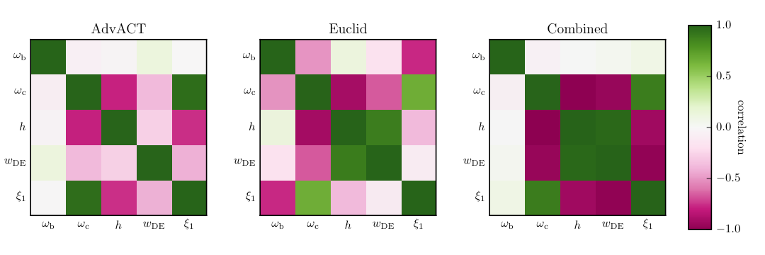
Confidence ellipses are shown in Fig. 9 for model 3, where we see in the middle and right-hand plots (as well as in Table 5) that CMB plays an important role in constraining , revealing that the interaction between DE and DM is already well constrained by CMB data before the inclusion of information about evolution. We can also see that for CMB alone in Fig. 10 (see the left-hand plot), the correlations are milder than for models 1 and 2. This agrees with the fact that for model 3, and are not degenerate at present times. In this case though, it appears that BAO does not help a lot to break remaining degeneracies. Indeed, all three combinations of parameters indicate a large correlation () when combining CMB and BAO probes.
The significance of the constraint on is already low at the current observational stage: Ref. [17] found (68% C. L.) when considering a combination of probes (Planck, SNIa, BAO, and data). Our forecast indicates that would yield (see Table 5), which would not improve the current best constraint much. However, one must be careful in doing this comparison because the current best constraint includes information from many other probes such as local measurements of the Hubble constant today and supernova data, which were not included in the forecast done here. For the model 3, it thus appears that a combination of other probes would still be needed in order to tighten the present limits.
V Summary and conclusions
We focused our study on phenomenological interacting DE models and investigated the impact of two probes on the parameter constraints of such models, specifically the primary CMB temperature and polarization spectrum and the BAO information from a redshift range of . The advantages of combining different observational probes in constraining cosmological parameters are well known, and its implication to interacting DE models has been widely addressed. Our motivation was to test the ability of future experiments to constraint such alternative scenarios and distinguish them from models in which there is no interaction in the dark sector.
For models 1 and 2 where the interaction is proportional to the DE energy density, stringent constraints were found in the dark sector parameters for the combined probes, especially for the coupling constant. Specifically, with the choice of fiducial values (model 1) and (model 2), we predicted 1- marginalized errors of at best (model 1) and (model 2). Thus, the combination of future CMB and BAO experiments, such as presented here, would probably be able to exclude the null interaction (corresponding to the CDM model) with a confidence level much greater than 3, although it is important to stress again that a proper statistical analysis will have to be done in order to really assess which model is preferred by the data. We also showed that the interacting DE models 1 and 2 are affected by degeneracies, which limits the constraining power of CMB information alone, but that they can be broken by the addition of Euclid-like BAO measurements, thus tightening the constraints on the dark sector cosmological parameters and enabling a deeper discussion of these interacting DE scenarios.
We found that the constraint on the coupling constant for model 3 (where interaction is proportional to the DM energy density) is not improved as much by the combination of future CMB and BAO experiments compared with its constraint derived by present datasets. It thus appears that extra information is still necessary for probing this model, and one could consider introducing the CMB lensing power spectra (possibly including higher order corrections [56]) and/or the convergence power spectrum from weak cosmic shear. We leave this investigation for future work.
We end by mentioning that future investigations of interacting DE could also benefit from yet more cosmological probes such as the redshift dependence of the Alcock-Paczyński effect [57], cosmic chronometers (see, e.g., Refs. [24, 58] and references therein), 21 cm cosmology (see, e.g., Refs. [59, 60] and references therein), gravitational waves [31, 34], and more. These examples of probes may be able to remove even more degeneracies and improve the constraints to another level and shall be considered in future work.
Acknowledgements.
We thank A. A. Costa for sharing his modified version of CAMB with us. LS and WZ are supported by the National Natural Science Foundation of China (NSFC) through grants Nos. 11603020, 11633001, 11173021, 11322324, 11421303, and 11653002. They are also supported by the project of Knowledge Innovation Program of Chinese Academy of Science, the Fundamental Research Funds for the Central Universities, and the Strategic Priority Research Program of the Chinese Academy of Sciences Grant No. XDB23010200. EF thanks CNPq (Science without Borders) for financial support. JQ acknowledges financial support from the Walter C. Sumner Memorial Fellowship and from the Vanier Canada Graduate Scholarship administered by the Natural Sciences and Engineering Research Council of Canada (NSERC). JQ also wishes to thank Yi-Fu Cai at USTC for hospitality when this work was initiated.Appendix A The elements of the CMB covariance matrix
In this appendix, we write down explicitly the elements of the CMB covariant matrix given in Eq. (16):
| (19) | ||||
| (20) | ||||
| (21) | ||||
| (22) | ||||
| (23) | ||||
| (24) |
In these equations, we defined , where and are the Gaussian random detector noises for temperature and polarization, respectively. One can express the random noises as follow,
| (25) | ||||
| (26) |
where the sums are over the frequencies () of the detector (see Table 2 for AdvACT). The window function is given by
| (27) |
and the inverse square of the detector noise level for temperature and polarization determines the weight given to each considered experiment channel (i.e., for each frequency ) [61]:
| (28) | ||||
| (29) |
where polarization sensitivities are rescaled by a factor of with respect to the temperature sensitivities, i.e., .
References
- [1] P. A. R. Ade et al. [Planck Collaboration], “Planck 2013 results. XVI. Cosmological parameters,” Astron. Astrophys. 571, A16 (2014) [arXiv:1303.5076 [astro-ph.CO]].
- [2] P. A. R. Ade et al. [Planck Collaboration], “Planck 2015 results. XIII. Cosmological parameters,” Astron. Astrophys. 594, A13 (2016) [arXiv:1502.01589 [astro-ph.CO]].
- [3] A. G. Riess et al. [Supernova Search Team], “Observational evidence from supernovae for an accelerating universe and a cosmological constant,” Astron. J. 116, 1009 (1998) [astro-ph/9805201]; “Type Ia supernova discoveries at from the Hubble Space Telescope: Evidence for past deceleration and constraints on dark energy evolution,” Astrophys. J. 607, 665 (2004) [astro-ph/0402512].
- [4] S. Perlmutter et al. [Supernova Cosmology Project Collaboration], “Measurements of Omega and Lambda from 42 high redshift supernovae,” Astrophys. J. 517, 565 (1999) [astro-ph/9812133].
- [5] P. Bull et al., “Beyond CDM: Problems, solutions, and the road ahead,” Phys. Dark Univ. 12, 56 (2016) [arXiv:1512.05356 [astro-ph.CO]].
- [6]
G. Bertone, D. Hooper and J. Silk,
“Particle dark matter: Evidence, candidates and constraints,”
Phys. Rept. 405, 279 (2005)
[hep-ph/0404175];
J. L. Feng, “Dark Matter Candidates from Particle Physics and Methods of Detection,” Ann. Rev. Astron. Astrophys. 48, 495 (2010) [arXiv:1003.0904 [astro-ph.CO]];
P. Scott, “Searches for Particle Dark Matter: An Introduction,” arXiv:1110.2757 [astro-ph.CO]. - [7]
S. Weinberg,
“The Cosmological Constant Problem,”
Rev. Mod. Phys. 61, 1 (1989);
M. Li, X. D. Li, S. Wang and Y. Wang, “Dark Energy,” Commun. Theor. Phys. 56, 525 (2011) [arXiv:1103.5870 [astro-ph.CO]]. - [8] I. Zlatev, L. M. Wang and P. J. Steinhardt, “Quintessence, cosmic coincidence, and the cosmological constant,” Phys. Rev. Lett. 82, 896 (1999) [astro-ph/9807002].
- [9]
D. Tocchini-Valentini and L. Amendola,
“Stationary dark energy with a baryon dominated era: Solving the coincidence problem with a linear coupling,”
Phys. Rev. D 65, 063508 (2002)
[astro-ph/0108143];
R. G. Cai and A. Wang, “Cosmology with interaction between phantom dark energy and dark matter and the coincidence problem,” JCAP 0503, 002 (2005) [hep-th/0411025];
X. Zhang, “Coupled quintessence in a power-law case and the cosmic coincidence problem,” Mod. Phys. Lett. A 20, 2575 (2005) [astro-ph/0503072];
M. S. Berger and H. Shojaei, “Interacting dark energy and the cosmic coincidence problem,” Phys. Rev. D 73, 083528 (2006) [gr-qc/0601086];
B. Hu and Y. Ling, “Interacting dark energy, holographic principle and coincidence problem,” Phys. Rev. D 73, 123510 (2006) [hep-th/0601093];
H. M. Sadjadi and M. Alimohammadi, “Cosmological coincidence problem in interactive dark energy models,” Phys. Rev. D 74, 103007 (2006) [gr-qc/0610080]. - [10]
L. P. Chimento, A. S. Jakubi, D. Pavón and W. Zimdahl,
“Interacting quintessence solution to the coincidence problem,”
Phys. Rev. D 67, 083513 (2003)
[astro-ph/0303145];
P. C. Ferreira, D. Pavón and J. C. Carvalho, “On detecting interactions in the dark sector with H(z) data,” Phys. Rev. D 88, 083503 (2013) [arXiv:1310.2160 [gr-qc]]. - [11] S. del Campo, R. Herrera and D. Pavón, “Toward a solution of the coincidence problem,” Phys. Rev. D 78, 021302 (2008) [arXiv:0806.2116 [astro-ph]]; “Interacting models may be key to solve the cosmic coincidence problem,” JCAP 0901, 020 (2009) [arXiv:0812.2210 [gr-qc]]; “Interaction in the dark sector,” Phys. Rev. D 91, no. 12, 123539 (2015) [arXiv:1507.00187 [gr-qc]].
- [12] B. Wang, Y. G. Gong and E. Abdalla, “Transition of the dark energy equation of state in an interacting holographic dark energy model,” Phys. Lett. B 624, 141 (2005) [hep-th/0506069].
- [13]
Y. Zhang, T. Y. Xia and W. Zhao,
“Yang-Mills condensate dark energy coupled with matter and radiation,”
Class. Quant. Grav. 24, 3309 (2007)
[gr-qc/0609115];
W. Zhao, “Attractor Solution and Coincidence Problems in Coupled Yang-Mills field Dark Energy Models,” Int. J. Mod. Phys. D 18, 1331 (2009) [arXiv:0810.5506 [gr-qc]]. - [14] J. H. He, B. Wang and E. Abdalla, “Testing the interaction between dark energy and dark matter via latest observations,” Phys. Rev. D 83, 063515 (2011) [arXiv:1012.3904 [astro-ph.CO]].
- [15] A. A. Costa, X. D. Xu, B. Wang, E. G. M. Ferreira and E. Abdalla, “Testing the Interaction between Dark Energy and Dark Matter with Planck Data,” Phys. Rev. D 89, no. 10, 103531 (2014) [arXiv:1311.7380 [astro-ph.CO]].
- [16] B. Wang, E. Abdalla, F. Atrio-Barandela and D. Pavón, “Dark Matter and Dark Energy Interactions: Theoretical Challenges, Cosmological Implications and Observational Signatures,” Rept. Prog. Phys. 79, no. 9, 096901 (2016) [arXiv:1603.08299 [astro-ph.CO]].
- [17] A. A. Costa, X. D. Xu, B. Wang and E. Abdalla, “Constraints on interacting dark energy models from Planck 2015 and redshift-space distortion data,” JCAP 1701, no. 01, 028 (2017) [arXiv:1605.04138 [astro-ph.CO]].
- [18] R. Murgia, S. Gariazzo and N. Fornengo, “Constraints on the Coupling between Dark Energy and Dark Matter from CMB data,” JCAP 1604, no. 04, 014 (2016) [arXiv:1602.01765 [astro-ph.CO]].
- [19]
V. Pettorino, L. Amendola, C. Baccigalupi and C. Quercellini,
“Constraints on coupled dark energy using CMB data from WMAP and SPT,”
Phys. Rev. D 86, 103507 (2012)
[arXiv:1207.3293 [astro-ph.CO]];
V. Pettorino, “Testing modified gravity with Planck: the case of coupled dark energy,” Phys. Rev. D 88, 063519 (2013) [arXiv:1305.7457 [astro-ph.CO]]. - [20]
V. Salvatelli, A. Marchini, L. Lopez-Honorez and O. Mena,
“New constraints on Coupled Dark Energy from the Planck satellite experiment,”
Phys. Rev. D 88, no. 2, 023531 (2013)
[arXiv:1304.7119 [astro-ph.CO]];
V. Salvatelli, N. Said, M. Bruni, A. Melchiorri and D. Wands, “Indications of a late-time interaction in the dark sector,” Phys. Rev. Lett. 113, no. 18, 181301 (2014) [arXiv:1406.7297 [astro-ph.CO]];
E. Di Valentino, A. Melchiorri and O. Mena, “Can interacting dark energy solve the tension?,” Phys. Rev. D 96, no. 4, 043503 (2017) [arXiv:1704.08342 [astro-ph.CO]]. - [21] W. Yang and L. Xu, “Cosmological constraints on interacting dark energy with redshift-space distortion after Planck data,” Phys. Rev. D 89, no. 8, 083517 (2014) [arXiv:1401.1286 [astro-ph.CO]]; “Testing coupled dark energy with large scale structure observation,” JCAP 1408, 034 (2014) [arXiv:1401.5177 [astro-ph.CO]]; “Coupled dark energy with perturbed Hubble expansion rate,” Phys. Rev. D 90, no. 8, 083532 (2014) [arXiv:1409.5533 [astro-ph.CO]].
- [22]
W. Yang, H. Li, Y. Wu and J. Lu,
“Cosmological constraints on coupled dark energy,”
JCAP 1610, no. 10, 007 (2016)
[arXiv:1608.07039 [astro-ph.CO]];
W. Yang, N. Banerjee and S. Pan, “Constraining a dark matter and dark energy interaction scenario with a dynamical equation of state,” Phys. Rev. D 95, no. 12, 123527 (2017) [arXiv:1705.09278 [astro-ph.CO]];
W. Yang, S. Pan and J. D. Barrow, “Large-scale Stability and Astronomical Constraints for Coupled Dark-Energy Models,” arXiv:1706.04953 [astro-ph.CO]. - [23]
Y. H. Li, J. F. Zhang and X. Zhang,
“Testing models of vacuum energy interacting with cold dark matter,”
Phys. Rev. D 93, no. 2, 023002 (2016)
[arXiv:1506.06349 [astro-ph.CO]];
R. Y. Guo, Y. H. Li, J. F. Zhang and X. Zhang, “Weighing neutrinos in the scenario of vacuum energy interacting with cold dark matter: application of the parameterized post-Friedmann approach,” JCAP 1705, no. 05, 040 (2017) [arXiv:1702.04189 [astro-ph.CO]]. - [24]
R. C. Nunes, S. Pan and E. N. Saridakis,
“New constraints on interacting dark energy from cosmic chronometers,”
Phys. Rev. D 94, no. 2, 023508 (2016)
[arXiv:1605.01712 [astro-ph.CO]];
S. Kumar and R. C. Nunes, “Echo of interactions in the dark sector,” Phys. Rev. D 96, no. 10, 103511 (2017) [arXiv:1702.02143 [astro-ph.CO]]. - [25] R. J. F. Marcondes, R. C. G. Landim, A. A. Costa, B. Wang and E. Abdalla, “Analytic study of the effect of dark energy-dark matter interaction on the growth of structures,” JCAP 1612, no. 12, 009 (2016) [arXiv:1605.05264 [astro-ph.CO]].
- [26] R. An, C. Feng and B. Wang, “Constraints on the dark matter and dark energy interactions from weak lensing bispectrum tomography,” JCAP 1710, no. 10, 049 (2017) [arXiv:1706.02845 [astro-ph.CO]].
- [27]
J. Q. Xia,
“New Limits on Coupled Dark Energy from Planck,”
JCAP 1311, 022 (2013)
[arXiv:1311.2131 [astro-ph.CO]];
J. S. Wang and F. Y. Wang, “Cosmological model of the interaction between dark matter and dark energy,” Astron. Astrophys. 564, A137 (2014) [arXiv:1403.4318 [astro-ph.CO]];
J. Väliviita and E. Palmgren, “Distinguishing interacting dark energy from wCDM with CMB, lensing, and baryon acoustic oscillation data,” JCAP 1507, no. 07, 015 (2015) [arXiv:1504.02464 [astro-ph.CO]];
D. M. Xia and S. Wang, “Constraining interacting dark energy models with latest cosmological observations,” Mon. Not. Roy. Astron. Soc. 463, no. 1, 952 (2016) [arXiv:1608.04545 [astro-ph.CO]];
C. van de Bruck, J. Mifsud and J. Morrice, “Testing coupled dark energy models with their cosmological background evolution,” Phys. Rev. D 95, no. 4, 043513 (2017) [arXiv:1609.09855 [astro-ph.CO]];
R. F. vom Marttens, L. Casarini, W. S. Hipólito-Ricaldi and W. Zimdahl, “CMB and matter power spectra with non-linear dark-sector interactions,” JCAP 1701 (2017) no.01, 050 [arXiv:1610.01665 [astro-ph.CO]];
R. Murgia, “Constraining the interaction between dark matter and dark energy with CMB data,” arXiv:1612.02282 [astro-ph.CO];
D. Bégué, C. Stahl and S. S. Xue, “A model of interacting dark fluids tested with supernovae data,” arXiv:1702.03185 [astro-ph.CO]. - [28] E. G. M. Ferreira, J. Quintin, A. A. Costa, E. Abdalla and B. Wang, “Evidence for interacting dark energy from BOSS,” Phys. Rev. D 95, no. 4, 043520 (2017) [arXiv:1412.2777 [astro-ph.CO]].
- [29] T. Delubac et al. [BOSS Collaboration], “Baryon acoustic oscillations in the Ly forest of BOSS DR11 quasars,” Astron. Astrophys. 574, A59 (2015) [arXiv:1404.1801 [astro-ph.CO]].
- [30]
L. Hollenstein, D. Sapone, R. Crittenden and B. M. Schäfer,
“Constraints on early dark energy from CMB lensing and weak lensing tomography,”
JCAP 0904, 012 (2009)
[arXiv:0902.1494 [astro-ph.CO]];
J. S.-Y. Leung and Z. Huang, “Marginalized Fisher Forecast for Horndeski Dark Energy Models,” Int. J. Mod. Phys. D 26, 1750070 (2017) [arXiv:1604.07330 [astro-ph.CO]];
I. Tutusaus, B. Lamine, A. Blanchard, A. Dupays, Y. Rousset and Y. Zolnierowski, “Dark sectors of the Universe: A Euclid survey approach,” Phys. Rev. D 94, no. 12, 123515 (2016) [arXiv:1607.08016 [astro-ph.CO]];
C. Heneka, D. Rapetti, M. Cataneo, A. B. Mantz, S. W. Allen and A. von der Linden, “Cold dark energy constraints from the abundance of galaxy clusters,” arXiv:1701.07319 [astro-ph.CO]. - [31] W. Zhao, C. Van Den Broeck, D. Baskaran and T. G. F. Li, “Determination of Dark Energy by the Einstein Telescope: Comparing with CMB, BAO and SNIa Observations,” Phys. Rev. D 83, 023005 (2011) [arXiv:1009.0206 [astro-ph.CO]].
- [32] L. Santos, P. Cabella, A. Balbi and N. Vittorio, “Neutrinos and dark energy constraints from future galaxy surveys and CMB lensing information,” Phys. Rev. D 88, no. 4, 043505 (2013) [arXiv:1307.2919 [astro-ph.CO]].
- [33]
M. Martinelli, E. Calabrese, F. De Bernardis, A. Melchiorri, L. Pagano and R. Scaramella,
“Constraining Modified Gravity with Euclid,”
Phys. Rev. D 83, 023012 (2011)
[arXiv:1010.5755 [astro-ph.CO]];
S. Casas, M. Kunz, M. Martinelli and V. Pettorino, “Linear and non-linear Modified Gravity forecasts with future surveys,” Phys. Dark Univ. 18, 73 (2017) [arXiv:1703.01271 [astro-ph.CO]]. - [34] C. Caprini and N. Tamanini, “Constraining early and interacting dark energy with gravitational wave standard sirens: the potential of the eLISA mission,” JCAP 1610, no. 10, 006 (2016) [arXiv:1607.08755 [astro-ph.CO]].
- [35] M. Martinelli, L. Lopez Honorez, A. Melchiorri and O. Mena, “Future CMB cosmological constraints in a dark coupled universe,” Phys. Rev. D 81, 103534 (2010) [arXiv:1004.2410 [astro-ph.CO]].
- [36] F. De Bernardis, M. Martinelli, A. Melchiorri, O. Mena and A. Cooray, “Future weak lensing constraints in a dark coupled universe,” Phys. Rev. D 84, 023504 (2011) [arXiv:1104.0652 [astro-ph.CO]].
- [37] L. Amendola, V. Pettorino, C. Quercellini and A. Vollmer, “Testing coupled dark energy with next-generation large-scale observations,” Phys. Rev. D 85, 103008 (2012) [arXiv:1111.1404 [astro-ph.CO]].
- [38] L. Amendola et al. [Euclid Theory Working Group], “Cosmology and fundamental physics with the Euclid satellite,” Living Rev. Rel. 16, 6 (2013) [arXiv:1206.1225 [astro-ph.CO]].
- [39] E. Calabrese et al., “Precision Epoch of Reionization studies with next-generation CMB experiments,” JCAP 1408, 010 (2014) [arXiv:1406.4794 [astro-ph.CO]].
- [40]
B. Wang, J. Zang, C. Y. Lin, E. Abdalla and S. Micheletti,
“Interacting Dark Energy and Dark Matter: Observational Constraints from Cosmological Parameters,”
Nucl. Phys. B 778, 69 (2007)
[astro-ph/0607126];
Z. K. Guo, N. Ohta and S. Tsujikawa, “Probing the Coupling between Dark Components of the Universe,” Phys. Rev. D 76, 023508 (2007) [astro-ph/0702015];
C. Feng, B. Wang, E. Abdalla and R. K. Su, “Observational constraints on the dark energy and dark matter mutual coupling,” Phys. Lett. B 665, 111 (2008) [arXiv:0804.0110 [astro-ph]];
T. Clemson, K. Koyama, G. B. Zhao, R. Maartens and J. Väliviita, “Interacting Dark Energy – constraints and degeneracies,” Phys. Rev. D 85, 043007 (2012) [arXiv:1109.6234 [astro-ph.CO]]. - [41] J. H. He and B. Wang, “Effects of the interaction between dark energy and dark matter on cosmological parameters,” JCAP 0806, 010 (2008) [arXiv:0801.4233 [astro-ph]].
- [42] J. H. He, B. Wang and E. Abdalla, “Stability of the curvature perturbation in dark sectors’ mutual interacting models,” Phys. Lett. B 671, 139 (2009) [arXiv:0807.3471 [gr-qc]].
- [43] Y. L. Bolotin, A. Kostenko, O. A. Lemets and D. A. Yerokhin, “Cosmological Evolution With Interaction Between Dark Energy And Dark Matter,” Int. J. Mod. Phys. D 24, no. 03, 1530007 (2015) [arXiv:1310.0085 [astro-ph.CO]].
- [44] M. Kunz, “The dark degeneracy: On the number and nature of dark components,” Phys. Rev. D 80, 123001 (2009) [astro-ph/0702615].
- [45] P. A. R. Ade et al. [Planck Collaboration], “Planck 2015 results. XIV. Dark energy and modified gravity,” Astron. Astrophys. 594, A14 (2016) [arXiv:1502.01590 [astro-ph.CO]].
- [46] L. Lopez Honorez, B. A. Reid, O. Mena, L. Verde and R. Jimenez, “Coupled dark matter-dark energy in light of near Universe observations,” JCAP 1009, 029 (2010) [arXiv:1006.0877 [astro-ph.CO]].
- [47] A. Lewis, A. Challinor and A. Lasenby, “Efficient computation of CMB anisotropies in closed FRW models,” Astrophys. J. 538, 473 (2000) [astro-ph/9911177].
- [48] G. Caldera-Cabral, R. Maartens and B. M. Schaefer, “The Growth of Structure in Interacting Dark Energy Models,” JCAP 0907, 027 (2009) [arXiv:0905.0492 [astro-ph.CO]].
- [49] H. J. Seo and D. J. Eisenstein, “Probing dark energy with baryonic acoustic oscillations from future large galaxy redshift surveys,” Astrophys. J. 598, 720 (2003) [astro-ph/0307460].
- [50] L. Wolz, M. Kilbinger, J. Weller and T. Giannantonio, “On the Validity of Cosmological Fisher Matrix Forecasts,” JCAP 1209, 009 (2012) [arXiv:1205.3984 [astro-ph.CO]].
- [51] M. Tegmark, “Measuring cosmological parameters with galaxy surveys,” Phys. Rev. Lett. 79, 3806 (1997) [astro-ph/9706198].
- [52] R. E. Smith et al. [VIRGO Consortium], “Stable clustering, the halo model and nonlinear cosmological power spectra,” Mon. Not. Roy. Astron. Soc. 341, 1311 (2003) [astro-ph/0207664].
- [53]
C. Carbone, M. Baldi, V. Pettorino and C. Baccigalupi,
“Maps of CMB lensing deflection from N-body simulations in Coupled Dark Energy Cosmologies,”
JCAP 1309, 004 (2013)
[arXiv:1305.0829 [astro-ph.CO]];
S. Casas, L. Amendola, M. Baldi, V. Pettorino and A. Vollmer, “Fitting and forecasting coupled dark energy in the non-linear regime,” JCAP 1601, no. 01, 045 (2016) [arXiv:1508.07208 [astro-ph.CO]];
V. Miranda, M. C. González, E. Krause and M. Trodden, “Finding structure in the dark: coupled dark energy, weak lensing, and the mildly nonlinear regime,” arXiv:1707.05694 [astro-ph.CO]. - [54] M. Zaldarriaga and U. Seljak, “An all sky analysis of polarization in the microwave background,” Phys. Rev. D 55, 1830 (1997) [astro-ph/9609170].
- [55] D. Coe, “Fisher Matrices and Confidence Ellipses: A Quick-Start Guide and Software,” arXiv:0906.4123 [astro-ph.IM].
- [56] G. Marozzi, G. Fanizza, E. Di Dio and R. Durrer, “CMB-lensing beyond the leading order: temperature and polarization anisotropies,” arXiv:1612.07263 [astro-ph.CO].
- [57] X. D. Li, C. Park, C. G. Sabiu, H. Park, D. H. Weinberg, D. P. Schneider, J. Kim and S. E. Hong, “Cosmological constraints from the redshift dependence of the Alcock-Paczynski effect: application to the SDSS-III BOSS DR12 galaxies,” Astrophys. J. 832, no. 2, 103 (2016) [arXiv:1609.05476 [astro-ph.CO]].
- [58]
R. Jimenez, L. Verde, T. Treu and D. Stern,
“Constraints on the equation of state of dark energy and the Hubble constant from stellar ages and the CMB,”
Astrophys. J. 593, 622 (2003)
[astro-ph/0302560];
D. Stern, R. Jimenez, L. Verde, M. Kamionkowski and S. A. Stanford, “Cosmic Chronometers: Constraining the Equation of State of Dark Energy. I: Measurements,” JCAP 1002, 008 (2010) [arXiv:0907.3149 [astro-ph.CO]];
M. Moresco, R. Jimenez, L. Verde, A. Cimatti, L. Pozzetti, C. Maraston and D. Thomas, “Constraining the time evolution of dark energy, curvature and neutrino properties with cosmic chronometers,” JCAP 1612, no. 12, 039 (2016) [arXiv:1604.00183 [astro-ph.CO]]. - [59]
R. Maartens et al. [SKA Cosmology SWG Collaboration],
“Overview of Cosmology with the SKA,”
PoS AASKA 14, 016 (2015)
[arXiv:1501.04076 [astro-ph.CO]];
R. Battye et al., “Update on the BINGO 21cm intensity mapping experiment,” arXiv:1610.06826 [astro-ph.CO]. - [60]
P. Bull, P. G. Ferreira, P. Patel and M. G. Santos,
“Late-time cosmology with 21cm intensity mapping experiments,”
Astrophys. J. 803, no. 1, 21 (2015)
[arXiv:1405.1452 [astro-ph.CO]];
K. Kohri, Y. Oyama, T. Sekiguchi and T. Takahashi, “Elucidating Dark Energy with Future 21 cm Observations at the Epoch of Reionization,” JCAP 1702, no. 02, 024 (2017) [arXiv:1608.01601 [astro-ph.CO]]. - [61] D. J. Eisenstein, W. Hu and M. Tegmark, “Cosmic complementarity: Joint parameter estimation from CMB experiments and redshift surveys,” Astrophys. J. 518, 2 (1999) [astro-ph/9807130].