Fractional chiral superconductors

Introduction.— Much is nowadays known about topological states which can be understood from a non-interacting limit. In this limit, the topological states protected by time-reversal, particle-hole, and chiral symmetries have been classified [1, 2]. Beyond this celebrated periodic table, topological phases protected by other symmetries such as lattice symmetries [3, 4, 5, 6, 7, 8, 9, 10, 11], have also been thoroughly studied.

In contrast, strongly interacting topologically ordered phases which cannot be understood in the absence of interactions, have yet to be fully understood and classified. Since interactions stabilize these phases, their study generally requires non-perturbative methods. A relatively recent approach to this problem is the coupled-wires approach [12, 13, 14, 15, 16, 17, 18, 19, 20, 21, 22, 23, 24, 25, 26, 27, 28, 29, 30, 31, 32], in which a two-dimensional (2D) or three-dimensional (3D) topologically ordered phase is constructed from an array of coupled quantum wires. The available machinery for studying interacting one-dimensional (1D) systems plays a central role in allowing one to write exactly solvable or analytically tractable model systems realizing such non-trivial phases of matter.

In this work we employ this approach to study fractional chiral superconductors (FCSC) in 2D. FCSC phases were previously introduced, mostly from a field-theoretic point of view, in Refs. [33, 34, 35]. The coupled-wires approach provides us with a tractable model which admits direct study of the properties of such phases.

We begin by constructing a non-interacting $p_{x}+ip_{y}$ topological superconductor (TSC). Following Ref. [15], this is done by placing an array of $N$ non-interacting weakly-coupled Rashba wires in proximity to an $s$-wave superconductor and applying a Zeeman field. We then add the effects of interactions and show that a fractional chiral superconductor (FCSC) can emerge at fractional filling factors, defined through the spin-orbit length (see Eq. 2). The main observation that will allow us to construct a model realizing the strongly-interacting FCSC phase is that, at fractional filling factors, one can define new local fermionic operators, composed of an electron dressed by a particle-hole excitation, for which the effective filling factor becomes an integer. Exploiting this fact, we will use the results of Ref. [15] to write a $p_{x}+ip_{y}$ topological superconductor in terms of the transformed fermions. Remarkably, in terms of the original fermions the resulting phase is a FCSC.

After constructing the model, we analyze it by mapping the low-energy theory of the individual wires at fractional fillings $\nu=1/m$ with odd $m$ to a generalized Sine-Gordon model. Performing an $\epsilon$-expansion for $m=2+\epsilon$, we show that each wire can be tuned to a $\mathbb{Z}_{2m}$ parafermion multicritical point [36]. We then demonstrate that one can couple different wires in such a way that a chiral $\mathbb{Z}_{2m}$ parafermion conformal field theory (CFT) is left on the edge (with $m$ being an odd integer, i.e., $\mathbb{Z}_{2},\mathbb{Z}_{6},\mathbb{Z}_{10},\cdots$ theories). By construction, the resulting 2D model is topologically ordered.

Our model allows us to study the physical properties of the FCSC phase. By considering a Corbino geometry (see Fig. 3a), we are able to study $h/2e$ vortices in the system. We show that these vortices host non-abelian parafermion zero-modes, by mapping our configuration to domain walls on the edge of a 2D fractional TI [37, 38, 39].

Finally, we examine the Josephson junction depicted in Fig. 1b, in which the superconductor stabilizing the FCSC is cut into two concentric annuli. In the quasi one-dimensional (thin annulus) regime, where coupling between the two edges is allowed, the radial Josephson current is shown to exhibit a $4\pi m$-periodicity as a function of the superconducting phase difference.

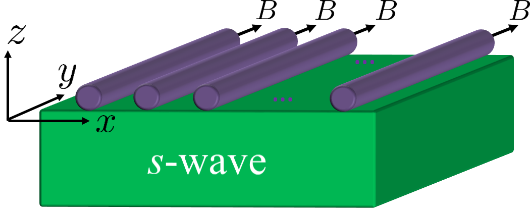
Topological superconductor from an array of coupled wires.— We start by reviewing the construction of a $p_{x}+ip_{y}$ superconductor, presented in Ref. [15]. The starting point is an array of decoupled Rashba wires. Similar to Refs. [40, 41], each wire is subjected to a Zeeman field and proximity coupled to an $s$-wave superconductor,

Here, $\vec{\psi}_{n}=\begin{bmatrix}\psi_{n\uparrow}(x)&\psi_{n\downarrow}(x)\end{bmatrix}^{T}$, where $\psi_{ns}(x)$ represents the electron annihilation operator at wire number $n$ with spin $s$ (see Fig. 1a). The matrices $\sigma_{i}$ are Pauli matrices operating on the spin degrees of freedom. The parameters $u,B,$ and $\Delta$ are the Rashba spin-orbit coupling (SOC), the Zeeman field, and the induced superconducting pairing potential, respectively.

Figure 2 presents the spectrum of a single wire in the absence of superconductivity and a Zeeman field ($B=\Delta=0$). We define the Fermi momentum $k_{F}^{0}=\sqrt{2M\mu}$ in the absence of SOC, and the shift $k_{\text{so}}=Mu$ of the parabolas due to SOC. In terms of these, the filling fraction of the system is defined as

To study the low energy physics, we linearize the spectrum near the Fermi level, and decompose the fermionic modes into right- and left-moving modes:

with $\psi_{ns\rho}(x)=\psi_{ns\rho}^{0}(x)e^{ik_{s\rho}x}$. Here, $\psi_{ns\rho}^{0}$ are the low energy degrees of freedom near the Fermi momenta $k_{s\rho}=\rho k_{F}^{0}-sk_{so}$ (where $\rho=\pm 1$ denotes a right/left moving mode).

The $p_{x}+ip_{y}$ superconductor corresponds to $\nu=1$. Focusing on the low-energy excitations for $\left|\Delta-B\right|\ll B,\Delta$, the Zeeman term $H_{B}=\int{\rm d}x\left[B\psi_{n\uparrow R}^{\dagger}(x)\psi_{n\downarrow L}(x)+{\rm h.c.}\right]$ and the pairing term $H_{\Delta}=\int{\rm d}x\left\{\Delta\left[\psi_{n\uparrow R}^{\dagger}(x)\psi_{n\downarrow L}^{\dagger}(x)+\psi_{n\uparrow L}^{\dagger}(x)\psi_{n\downarrow R}^{\dagger}(x)\right]+{\rm h.c.}\right\}$ gap out the wires (see Fig. 2). Indeed, the second term in $H_{\Delta}$ fully gaps the high-momentum degrees of freedom $\psi_{n\uparrow L}$ and $\psi_{n\downarrow R}$, and the low-momentum degrees of freedom, $\psi_{n\uparrow R}$ and $\psi_{n\downarrow L}$, are coupled by the Zeeman term $H_{B}$ as well as the first term of $H_{\Delta}$. The fully gapped phases for $\Delta>B$ and $\Delta<B$ are topologically distinct - the first is a 1D trivial phase while the second is a topological superconductor. For $B=\Delta$, the inter-mode part of the Hamiltonian, given by $H_{\Delta}+H_{B}$, commutes with the operators

so the system is gapless.

Tuning to this transition point, we introduce an inter-wire term of the form

This term arises naturally in the system of Fig. 1a due to a combination of inter-wire hopping, superconductivity, and spin-orbit interaction [15]. It gaps out the bulk degrees of freedom, yet it leaves the Majorana fields $\beta_{1}(x)\text{ and }\alpha_{N}(x)$ decoupled, thus stabilizing a $p_{x}+ip_{y}$ TSC phase. This construction can be considered the anisotropic limit of the system studied by Refs. [42, 43]. While it relies on a fine-tuned relation between parameters, the resulting phase is independent of these assumptions, remaining qualitatively identical as long as the bulk gap remains open.

Fractional chiral superconductors.— To construct a FCSC phase at filling $\nu=1/m$, we consider the effects of strong interactions, within a bosonized description of the 1D degrees of freedom. Using the standard Abelian bosonization technique, we describe the Hilbert space in terms of bosonic fields $\phi_{ns\rho}$ via $\psi_{ns\rho}\propto e^{i\left(\phi_{ns\rho}+k_{s\rho}x\right)}$. The boson fields satisfy the commutation relations

where $A_{ns\rho}^{n^{\prime}s^{\prime}\rho^{\prime}}$ takes the values $\pm 1$ for any $\left\{ns\rho\right\}\neq\left\{n^{\prime}s^{\prime}\rho^{\prime}\right\}$ and is antisymmetric with respect to the exchange $\left\{ns\rho\right\}\leftrightarrow\left\{n^{\prime}s^{\prime}\rho^{\prime}\right\}$ (ensuring that the fermionic anti-commutation relations are satisfied).

For $\nu=1/m$, it is useful to define new chiral fermion operators $\tilde{\psi}_{ns\rho}=e^{i\left(\eta_{ns\rho}+q_{s\rho}x\right)}$, with

The new fields, $\tilde{\psi}_{ns\rho}$, are fermionic, as evident from the commutation relations

where $\tilde{A}_{ns\rho}^{n^{\prime}s^{\prime}\rho^{\prime}}$ takes odd integer values for any $\left\{ns\rho\right\}\neq\left\{n^{\prime}s^{\prime}\rho^{\prime}\right\}$, and is antisymmetric with respect to the exchange $\left\{ns\rho\right\}\leftrightarrow\left\{n^{\prime}s^{\prime}\rho^{\prime}\right\}$. The $\tilde{\psi}_{ns\rho}$ fields carry momenta $q_{s\rho}=\frac{m+1}{2}k_{s\rho}-\frac{m-1}{2}k_{s\bar{\rho}}.$

Note that the momenta $q_{s\rho}$ carried by the new fields $\tilde{\psi}_{ns\rho}$ match those of a $\nu=1$ wire. In particular, the operators $\tilde{\psi}_{n\uparrow R}$ and $\tilde{\psi}_{n\downarrow L}$ now have vanishing oscillatory components, allowing us to couple them in various ways without breaking translational symmetry.

Once the Zeeman term is dressed by intra-wire $2k_{F}$-interactions, it induces a term of the form $\tilde{H}_{B}=\int\frac{{\rm d}x}{a^{2}}\left[\tilde{B}\tilde{\psi}_{n\uparrow R}^{\dagger}(x)\tilde{\psi}_{n\downarrow L}(x)+{\rm h.c.}\right]$ (where $a$ is the short distance cutoff). We assume that $\tilde{B}$ is large enough such that this term gaps out the small momentum fields $\tilde{\psi}_{n\uparrow R}\text{ and }\tilde{\psi}_{n\downarrow L}$. We may also write dressed pairing terms of the form $\tilde{H}_{\Delta}=\int\frac{{\rm d}x}{a^{2}}\left\{\tilde{\Delta}\left[\tilde{\psi}_{n\uparrow R}^{\dagger}(x)\tilde{\psi}_{n\downarrow L}^{\dagger}(x)+\tilde{\psi}_{n\uparrow L}^{\dagger}(x)\tilde{\psi}_{n\downarrow R}^{\dagger}(x)\right]+{\rm h.c.}\right\}$. As in the $\nu=1$ case, the second term in $\tilde{H}_{\Delta}$ involves high-momentum degrees of freedom and does not compete with the Zeeman term, $\tilde{H}_{B}$. It fully gaps out the fields $\tilde{\psi}_{n{\uparrow}L}$ and $\tilde{\psi}_{n{\downarrow}R}$. The first term in $\tilde{H}_{\Delta}$ competes with the Zeeman field $\tilde{H}_{B}$. For $\tilde{\Delta}=\tilde{B}=\lambda$, one obtains a critical theory, similar to the $\nu=1$ case, which in this case is described by a $\beta^{2}=4\pi m$ self-dual Sine-Gordon model (see Appendix A):

where we have defined $\varphi=\frac{\eta_{n\uparrow R}-\eta_{n\downarrow L}}{2\sqrt{\pi m}}$ and $\theta=\frac{\eta_{n\uparrow R}+\eta_{n\downarrow L}}{2\sqrt{\pi m}}$.

It is, however, a priori unclear whether the critical line $\tilde{B}=\tilde{\Delta}$ is dominated by the $\tilde{B}$ and $\tilde{\Delta}$ terms. In the weak-coupling limit, both $\tilde{B}$ and $\tilde{\Delta}$ flow to zero, giving a trivial Luttinger-liquid fixed point. However, it turns out that when $\tilde{B}$ and $\tilde{\Delta}$ are equal and large enough, a non-trivial multicritical point is encountered.

To show this, we follow the analysis in Ref. [44], and employ an $\epsilon$-expansion, with $m=2+\epsilon$. In this approach, the scaling dimensions of the $\tilde{B}$ and $\tilde{\Delta}$ terms are small, thus pushing the competition between the first and higher order terms of the RG equations to the region in which the perturbative RG analysis applies. As we show in Appendix A, the RG equation describing the flow of $\lambda=\tilde{B}=\tilde{\Delta}$ takes the form

When $\lambda>\sqrt{\epsilon}/\pi$, a flow to large coupling ensues and the low energy theory is no longer capable of describing the model. The point $\lambda=\sqrt{\epsilon}/\pi$ is a multicritical point separating the $\tilde{B}$-dominated phase, the $\tilde{\Delta}$-dominated phase, and the gapless phase. Extrapolating to $\epsilon$ of order unity, we assume that such a critical point persists. For completeness, we study the full phase diagram of the system in Appendix A.

To uncover the nature of the CFT describing the multicritical point, it is useful to review the physics of classical 2D $\mathbb{Z}_{k}$ (clock or Potts) models. As discussed in detail in Refs. [45, 46, 47], such models possess self-dual lines. For $k\leq 4$, there is a self-dual critical point that separates the disordered and ordered ($\mathbb{Z}_{k}$ symmetry broken) phases. For $k>4$, some regions of the self-dual line are contained in gapless phases, while others consist of first order transitions. The different regions of the self-dual line are separated by multicritical points [45, 47]. It was argued in Ref. [36] that these are described by a $\mathbb{Z}_{k}$ parafermion CFT. In addition, it is well known that the low energy physics of self-dual $\mathbb{Z}_{k}$ models is described by $\beta^{2}=2\pi k$ self-dual Sine-Gordon models [48, 49]. The above prompts us to identify the finite-coupling multicritical point in our self-dual Sine-Gordon models with those of the $\mathbb{Z}_{k}$ models. This indicates that our model at the multicritical point is described by a $\mathbb{Z}_{2m}$ parafermion CFT.

In what follows, we assume that each wire is tuned to the multicritical point, and is therefore described by a $\mathbb{Z}_{2m}$ parafermion theory. At this critical point, the fields

commute with the inter-mode Hamiltonian $\tilde{H}_{B}+\tilde{H}_{\Delta}$. As we demonstrate in Appendix B, the propagators describing this low energy theory take the form $\left\langle\tilde{\alpha}_{n}(z)\tilde{\alpha}_{n}(z^{\prime})\right\rangle\propto\left(z-z^{\prime}\right)^{-m}$ and $\left\langle\tilde{\beta}_{n}(\bar{z})\tilde{\beta}_{n}(\bar{z}^{\prime})\right\rangle\propto\left(\bar{z}-\bar{z}^{\prime}\right)^{-m}$, with $z=x+i\tau$. We identify these fields with the $\psi_{m}$ and $\bar{\psi}_{m}$ primary fields of the $\mathbb{Z}_{2m}$ theory, which indeed have conformal dimension $m/2$ [36].

Similar to the non-interacting case [see Eq. (5)], we introduce the inter-wire term

Since the inter-wire Hamiltonian in Eq. (12) has the same form as the self-dual intra-wire Hamiltonian and is composed of fields which commute with the intra-wire coupling terms, $\tilde{t}_{\perp}$ flows according to the RG equation (10). Therefore, if $\tilde{t}_{\perp}$ is large enough, a flow to large coupling ensues and this Hamiltonian leaves the fields $\tilde{\beta}_{1}$ and $\tilde{\alpha}_{N}$ gapless. These fields represent the local electron operators on the edges. In fact, a full chiral $\mathbb{Z}_{2m}$ parafermion CFT is expected to reside on each edge. Using the propagator of the $\tilde{\alpha}$ and $\tilde{\beta}$ fields, we find that the electrons’ tunneling density of states $N(\omega)$, associated with the edge, scales with an anomalous exponent: $N(\omega)\propto\omega^{m-1}$.

Similar to the non-interacting case, the strict constraints on the various parameters may be lifted as long as the bulk gap does not close.

Non-abelian defects and $4\pi m$-periodic Josephson effect.— To study the non-Abelian defects residing at the core of vortices, we examine the configuration presented in Fig. 3a. The FCSC is shaped like an annulus, and the flux threading the annulus is given by an odd multiple of $h/2e$ ¹¹ 1 We note that depending on the specific details of the model, the role of even and odd number of vortices may interchange.. In analogy to the non-interacting case [50], we expect to find zero modes on the two edges of the system. It will prove useful to cut a thin trench in the annulus. In this case, the flux through the center of the annulus can be chosen to enter in the coupling across the trench, and we can deform our system in such a way that connects it with the configuration studied in Refs. [37, 38, 39] (see Fig. 3f).

Given that we are only interested in finding zero energy modes, we have a large amount of freedom in deforming the geometry of the problem while preserving its topology. We first fold the edge “inside-out” leading to the bone-shaped configuration depicted in Fig. 3b. We may then shrink the outermost regions without introducing inter-edge coupling. This leads to the simple 1D geometry presented in Fig. 3c, in which the counter-propagating edge modes $\tilde{\alpha}_{R}$ and $\tilde{\beta}_{L}$ (defined in the region $0<x<l$) are connected at $x=0,l$.

The zero-mode properties are solely encoded in the low energy edge theory. We therefore have the additional freedom of changing the Hamiltonian governing the gapped degrees of freedom. One must only ensure that the modes $\tilde{\alpha}_{R}$ and $\tilde{\beta}_{L}$, and the other primary fields of the parafermion CFT, remain gapless, while the other microscopic degrees of freedom, such as $\tilde{\alpha}_{L}$ and $\tilde{\beta}_{R}$, remain gapped.

An auxiliary model, in which the latter fields are coupled directly, while bulk degrees of freedom are projected out, satisfies this condition. The corresponding Hamiltonian is given by

where we have used $\tilde{\alpha}_{\rho}=\tilde{\psi}_{\rho}+\tilde{\psi}_{\rho}^{\dagger}$ and $\tilde{\beta}_{\rho}=\left(\tilde{\psi}_{\rho}-\tilde{\psi}_{\rho}^{\dagger}\right)/i$. While it gaps $\tilde{\alpha}_{L}$ and $\tilde{\beta}_{R}$, this Hamiltonian leaves the fields $\tilde{\alpha}_{R},\tilde{\beta}_{L}$ gapless. Notice that strictly speaking, $\tilde{t}_{\rm{a}}$ must be tuned to a multicritical point for the low-energy theory to remain identical. However, since we will soon break the self duality of the problem, this will not be important.

The auxiliary model simplifies our analysis, as it allows us to formulate the problem in terms of the chiral bosonic modes $\eta_{R}$ and $\eta_{L}$, such that $\tilde{\psi}_{\rho}=e^{i\eta_{\rho}}$. Mathematically, the Hamiltonian in Eq. (13) describes two edge modes of a $\nu=1/m$ fractional quantum Hall state, coupled by a specific combination of ferromagnetic and superconducting terms.

Next, we include the physical coupling between the edge modes across the trench,

where $\varphi=2\pi\frac{\Phi}{h/2e}$, and $\Phi=nh/2e$ is the flux through the center of the annulus. In the gauge in which the flux only enters into $\tilde{t}\left(\varphi\right)$, we have $\tilde{t}\left(\varphi\right)=\tilde{t}_{0}\cos\left(\frac{\varphi}{2}\right)$.

Finally, it is necessary to introduce the correct boundary conditions, such that $\tilde{\alpha}_{R}\rightarrow\tilde{\beta}_{L}$ at $x=0$ and $\tilde{\beta}_{L}\rightarrow\tilde{\alpha}_{R}$ at $x=l$ (see Fig. 3c). This can be implemented by extending the model to $-\infty<x<\infty$, and strongly coupling $\alpha_{R}$ and $\beta_{L}$ beyond the ends of the physical system, such that they acquire a large gap in these regions. Within the auxiliary model, formulated in terms of the two $\eta$ fields, we can do this by introducing strong superconducting terms for $x<0$ and $x>l$:

The full auxiliary model is depicted in Fig. 3d. Alternatively, note that one can also use a ferromagnetic term. This would not change our conclusions regarding the existence of zero modes.

While the choice of coupling constants $\tilde{t}_{a}$ and $\Delta_{\rm bc}$ seems arbitrary, unphysical zero energy degrees of freedom may appear if these are not properly chosen. In order to avoid these, we first choose the auxiliary coupling constant such that $\sgn\left(\tilde{t}_{a}\right)=\sgn\left(\Delta_{\rm bc}\right)$ (otherwise the coefficient of the term $i\tilde{\beta}_{R}\tilde{\alpha}_{L}$ changes sign at $x=0,l$).

An additional consistency condition is obtained by noting that no physical zero-energy modes should appear in the absence of flux. This leads to the constraint $\sgn\left(\Delta_{\rm bc}\right)=\sgn\left[\tilde{t}\left(\varphi=0\right)\right]$.

To be consistent with these constraints, the coefficients of our auxiliary model must satisfy

Clearly, the gap does not close as long as the various coupling constants do not change sign. In particular, the presence (or absence) of zero-modes in not affected by varying the various parameters without altering their signs. We may therefore choose $\tilde{t}_{0}=\tilde{t}_{a}\left|\cos\left(\frac{\varphi}{2}\right)\right|^{-1}$, in which case the Hamiltonian in the region $0<x<l$ takes the form

While the trench allows us to continuously vary $\varphi$, we take the discrete values $\varphi=2\pi n$, where $n$ counts the number of $h/2e$ vortices. As Eq. (17) implies, if $\varphi$ is an even multiple of $2\pi$, the Hamiltonian reduces to superconducting terms throughout space, thus preventing the existence of zero energy modes (see Fig. 3e). On the other hand, if $\varphi$ is an odd multiple of $2\pi$ it is clear that the superconductor in the region $0<x<l$ is replaced by a ferromagnet, and we end up with the S-F-S configuration studied in Refs. [37, 38, 39] (see Fig. 3f). Notice that if we had chosen to implement the boundary conditions in Eq. (15) using ferromagnetic terms, we would end up with an F-S-F configuration for odd multiples of $2\pi$, and ferromagnetic terms throughout space for even multiple of $2\pi$.

Following the results of Refs. [37, 38, 39], we conclude that the S-F-S and F-S-F configurations found above give rise to parafermion zero-modes $\xi_{i}$, with $i=1,2$, located at the interfaces $x=0,l$. These operators satisfy

and $\xi_{i}^{2m}=1$. Eq. (17) implies that the spectrum is $4\pi$-periodic as a function of $\varphi$.

We note that the interfaces correspond to the circular edges of the original annulus, so that this line of arguments indicates that $h/2e$ vortices in the FCSC system bind protected parafermionic zero-modes. The parafermion nature of these excitations provides a natural generalization to the case where the bulk contains many vortices, each binding a zero-mode generated by $\xi_{i}$ ($i=1\cdots 2M$ is an arbitrary index labeling the zero-modes). The parafermions generally satisfy the algebra

from which one can infer a ground state degeneracy of $\left(2m\right)^{M}$ for $2M$ vortices.

Once our annular system is transformed into the setup presented in Fig. 3f for an odd number of vortices, it is natural to ask whether we can control the relative phase between the two effective superconducting order-parameters and measure the Josephson effect, which was previously shown to be $4\pi m$-periodic [38, 39].

Recall that the superconductors shown in Fig. 3f were introduced to impose the boundary conditions, and in particular, do not correspond to the physical superconductor in proximity to our system. Nevertheless, we argue that such an effective Josephson junction can be generated by creating a physical Josephson junction in our system. This is done by considering a physical weak link cutting the physical superconductor at a fixed radial coordinate into two concentric annuli (see Fig. 1b). This allows us to control the relative superconducting phases between the external and the internal parts of our system by connecting the two edges with an external superconducting wire, through which flux is inserted.

Since the edges of our annular system correspond to the interfaces in the auxiliary configuration, we effectively control the relative phases between the two auxiliary superconductors shown in Fig. 3f ²² 2 Notice that the phase differences in the effective and the physical Josephson junctions play a similar role in changing the wave function of the low energy electron operators. This indicates that changing the phase difference in the physical junction results in a phase difference in the effective junction as well. . Examining the quasi one dimensional regime, in which coupling between the two edge modes of our annular system is induced, the arguments above indicate that the junction shown in Fig. 1b gives rise to a $4\pi m$-periodic Josephson effect.

Conclusion.— In this work we have demonstrated that a FCSC phase can be stabilized in an array of coupled wires in the presence of Rashba SOC, Zeeman field, superconducting proximity effects, and strong interactions. The resulting phase was found to give rise to a parafermionic edge theory, whose central charge is $c=\frac{2m-1}{m+1}$. In this theory, the electron has an anomalous tunneling density of states of the form $N(\omega)\propto\omega^{m-1}$. We have additionally found that $h/2e$ vortices in such a system bind parafermionic zero modes, with quantum dimension $\sqrt{2m}$.

Clearly, the FCSC phase we construct is topologically ordered. While we leave the detailed study of the bulk excitations to future studies, we anticipate that the topologically distinct bulk excitations will be associated with the various low-energy sectors of the parafermionic edge theory through the bulk-edge correspondence. The low energy sectors are generated by the primary fields of the parafermion CFT, which can be labeled by $\Phi_{[k,\bar{k}]}$ [36], where the integers $k$ and $\bar{k}$ are defined mod $4m$, and $k+\bar{k}$ is even. In terms of these, the parafermion fields are given by $\psi_{n}=\Phi_{[2n,0]}$ and $\bar{\psi}_{n}=\Phi_{[0,2n]}$ (with $n=1,\cdots,2m-1$), and the spin operators $\sigma_{n}$ are given by $\sigma_{n}=\Phi_{[n,n]}$.

However, in identifying the deconfined bulk excitations with the primary fields of the edge CFT, we must exclude the operators which acquire a non-trivial phase as they wind around the electron, which in our case is identified with the field $\psi_{m}$ (or $\bar{\psi}_{m}$). In particular, since the electron acquires a phase of $\pi$ as it winds around a vortex, the corresponding field must be associated with a confined excitation (i.e., the energy of two such excitations diverges as we separate them ³³ 3 Notice that such confined excitation can be introduced to the system externally. For example, a vortex in a $p_{x}+ip_{y}$ superfluid is confined, but it can be induced by applying an external effective magnetic field. ). More generally, the phase associated with winding $\Phi_{[k,\bar{k}]}$ around the electron $\psi_{m}$ ($\bar{\psi}_{m}$) is given by $\gamma_{[k,\bar{k}]}=\pi k$ ($\bar{\gamma}_{[k,\bar{k}]}=\pi\bar{k}$) [36]. This shows, for example, that while the parafermion fields $\psi_{n}$ are all deconfined in the bulk, the spin operators $\sigma_{n}$, with odd $n$, must be confined.

It has recently been shown that repulsive interactions can stabilize a time reversal invariant topological superconducting (TRITOPS) phase in quantum wires [51, 52, 53, 54, 55, 56]. It would be interesting to consider an array of such 1D systems as a possible realization of a fractional TRITOPS in 2D.