Our starting point is Chern-Simons theory defined on $S^{2}\times(-\infty,0]\sim B^{3}$ with the two-sphere being punctured by $n$-pairs of quasi-particles/holes. The particles’ trajectories admit a topological classification in terms of a braid description which define the density matrix associated with the system. In the Lorentzian picture, the 3-ball topology arises from taking time $t\in(-\infty,0]$ and space to be the two-sphere. After pair creation of quasi-particles which carry non-trivial quantum statistics in Chern-Simons theory, one ends up with the topologically equivalent description of a boundary two-sphere punctured with the quasi-particles and connected by braided Wilson lines that extend in the interior of the three-ball.

As was first explained in Witten’s seminal work [11], the path-integral of Chern-Simons theory on the three-ball $B^{3}$ yields a state $|\varphi\rangle$ living on the boundary $S^{2}$. Given a braid diagram connecting the quasi-holes on the bottom with the quasi-particles on top (we fix the orientation such that the Wilson lines flow from the bottom to top in the braid diagram corresponding to the state ket ), one can associate with it a state vector $|\varphi\rangle$ as well as a dual state $\langle\varphi|$ defined by switching the particles with holes, and the nature of the crossings in the braid diagram as sketched in Fig. 1.

To relate it to a braid description, we can associate $|\varphi\rangle$ and $\langle\varphi|$ with braid words of some length $m$ respectively as

	$\displaystyle b_{|\varphi\rangle}=\prod^{m}_{i=1}\sigma^{s_{i}}_{f(i)},$		(2.1)
	$\displaystyle b_{\langle\varphi|}=\prod^{m}_{i=1}\sigma^{-s_{i}}_{n-f(i)}.$		(2.2)

where $s_{i}\in\mathbb{Z}$, $n$ is the number of pairs of quasi-particles and $\sigma_{k}$ refers to the $k^{\text{th}}$ string overcrossing the $(k+1)^{\text{th}}$ string. We note that in the standard narrative that relates braids and links, if we close the braids after fixing a braid axis and obtain the link then the link associated with $\langle\varphi|$ has opposite orientation and is also a mirror image of the original link associated with $|\varphi\rangle$.

We are now ready to define the density matrix in terms of an auxiliary link in $S^{3}$. Consider a bipartition of the system into two subsystems defined by picking a region containing a proper subset of the particles/holes. Let $R_{\mathcal{B}}$ be a set of discs containing some quasi-particles/holes, then the partial density matrix obtained after tracing over $\mathcal{B}$, i.e. $\rho_{A}=\text{Tr}_{B}|\varphi\rangle\langle\varphi|$ is represented by the auxiliary link obtained by joining $n$ copies of this pair of diagram in the following manner: (i) connecting region $\mathcal{B}$ between the diagrams associated with the ket and bra in each factor of³³ 3 Henceforth, we would let $\rho$ denote the reduced density matrix $\rho_{\mathcal{A}}$, with $\mathcal{B}$ being the region that is traced over. $\rho_{\mathcal{A}}=\rho=|\varphi\rangle\langle\varphi|$, thus perfoming the partial trace (ii) connecting the complementary region $R_{\mathcal{A}}$ between each neighboring pair of $\{\langle\varphi|,|\varphi\rangle\}$. We are then left with two residual regions $R_{\mathcal{A}}$ in the first ket $|\varphi\rangle$ and last bra $\langle\varphi|$, as sketched in Fig. 2.

This gluing procedure has an equivalent description of a Chern-Simons path-integral on a 3-manifold that is topologically a 3-ball with punctures. Finally, tracing over the reduced density matrix implies that we identify the remaining boundary areas to obtain an $S^{3}$ that contains the auxiliary link formed after connecting the punctures in the above fashion. This yields the Renyi entropy after normalizing $\text{Tr}(\rho^{n})$ by $(\text{Tr}\,\rho)^{n}$. By invoking the replica trick, the entanglement entropy follows immediately.

In this paper, we will let $\mathcal{L}_{n}$ denote the auxiliary link associated with $\text{Tr}\,(\rho^{n})$ and let $\langle\mathcal{L}_{n}\rangle$ refer to its Kauffman bracket which is, up to a gauge group-dependent factor, the Chern-Simons VEV of the link. Following standard knot theory literature nomenclature, we set the Kauffman bracket of the unknot to be unity. We also let the Wilson lines to be in the fundamental representation of $SU(2)_{k}$ Chern-Simons theory, and thus we can write

$$Z\left(\mathcal{L}_{n}\right)=\text{Tr}\,(\rho^{n})=\langle\mathcal{L}_{n}\rangle\,S_{0\frac{1}{2}}$$

(2.3)

where $Z\left(\mathcal{L}_{n}\right)$ is the partition function of Chern-Simons theory with the auxiliary link inserted in $S^{3}$, $S_{ij}=\sqrt{\frac{2}{k+2}}\sin\left(\frac{\pi(2i+1)(2j+1)}{k+2}\right)$ is the modular S-matrix. It arises in (2.3) because $Z(\text{unknot})=S_{0\frac{1}{2}}$. The Renyi and entanglement entropies then follow to read

	$\displaystyle S^{(n)}_{R}$	$\displaystyle=$	$\displaystyle\text{Log}\,S_{0\frac{1}{2}}+\frac{1}{1-n}\text{Log}\left(\frac{\langle\mathcal{L}_{n}\rangle}{\langle\mathcal{L}_{1}\rangle^{n}}\right),$		(2.4)
	$\displaystyle S_{EE}$	$\displaystyle=$	$\displaystyle\text{Log}\,(\langle\mathcal{L}_{1}\rangle S_{0\frac{1}{2}})-\frac{1}{\mathcal{L}_{1}}\partial_{n}\langle\mathcal{L}_{n}\rangle|_{n=1}.$		(2.5)

In the seminal work of [5], it was first explained that topological entanglement entropy in Chern-Simons theory probes the braiding of quasi-particles in an elegant fashion that relates to fusion rules and conformal blocks of the associated WZW conformal field theory living on the spatial two-sphere. This analysis was carried further in [6] where a connection to edge states and R-matrices (in the language of modular tensor category) was demonstrated. In both papers, the sensitivity to braiding was essentially captured by using a linear combination of states for $|\varphi\rangle$, notably with the discussion restricted to two pairs of quasi-particles and pertaining to a few choices of the regions $R_{\mathcal{B}}$.

The possibly much richer narrative that we outlined above was however not quite explored previously. If we take $R_{\mathcal{B}}$ to enclose all the holes (or all the particles), then the gluing procedure is identical to the usual braid multiplication via concatenation, the end result being the standard closure of the braid word $(b_{|\varphi\rangle}b_{\langle\varphi|})^{n}$ which by virtue of (2.1) and (2.2) is nothing but the identity braid.⁴⁴ 4 Note that when $\mathcal{R}_{B}$ encloses all quasi-particles, the gluing is represented by concatenating the braid $\langle\varphi|$ with the strand index reversed, i.e. $k\rightarrow n-k$ in $\sigma_{k}$ of (2.2).

This implies that Renyi entropy vanishes for all $n$. There are however other possible choices of $R_{\mathcal{B}}$ which furnish non-vanishing entanglement measures. Hence, without alluding to a linear combination of states associated with distinct braids, the entanglement entropy is generically a non-trivial function of the braid geometry. This furnishes a simple setting where one could relate between the notion of quantum entanglement and elements of braid theory.

For the rest of the paper, we shall embark on an exploration of how, equipped with some suitable choices of the region $R_{\mathcal{B}}$, the entanglement entropies probe the geometric complexity of braided configurations of quasi-particles and distinguish between different braids. Associated with a braid is the link obtained by its closure so it is useful to organize various braid configurations according to their geometrical interpretation as the braid presentations for various links. Nonetheless, as we shall elaborate in detail shortly, the entanglement measures change under Markov moves and we could generically have different entanglement entropies for a pair of braids equivalent up to the two type of Markov moves of stabilization and conjugation.

There is a subtlety that arises for picking a certain $R_{\mathcal{B}}$, that comes with performing the gluing procedure. Let’s recall that a standard surgery procedure in $S^{3}$ involves removing and gluing back a solid torus which is the toroidal neighborhood of some link with a possibly non-trivial homeomorphism of the boundary torus valued in the mapping class group of $T^{2}$. In our context, we are gluing together a set of punctured discs and identifying punctures. The gluing procedure can be decomposed into two steps - one that translates to taking the partial trace over $R_{\mathcal{B}}$ and the other one corresponding to the field operator product of $\rho$.

It is convenient, as we have illustrated in Fig. 2 to order the punctures in a line. Consider the case where some quasi-particles of $R_{\mathcal{B}}$ lie on the right of those in $R_{\mathcal{A}}$ in the diagram corresponding to $\langle\varphi|$ (see Fig. 1) Now, for every hole in $R_{\mathcal{A}}$, one identifies it with the corresponding particle in the neighboring diagram associated with $|\varphi\rangle$. The gluing is done by connecting the pair with a Wilson line, which then has to cross all the lines connecting the particles in region $R_{\mathcal{B}}$. The choice of either overcrossing or undercrossing is to be made for every Wilson line crossed. Thus, in general, the gluing procedure that identifies the copies of $R_{\mathcal{A}}$’s in each neighboring pair of ket and bra is accompanied with an indication of the choice of crossings among the Wilson lines whenever such ambiguity arises.

We could keep track of any choice by indicating a braid word for each quasi-particle in any subregion of $R_{\mathcal{B}}$ that lies on the right of those in $R_{\mathcal{A}}$ for $\langle\varphi|$. But for the rest of the paper, we will not discuss this subtlety further. Our working examples involve choices of the region $R_{\mathcal{B}}$ such that the auxiliary link can be constructed uniquely once we indicate the quasi-particles/holes that $R_{\mathcal{B}}$ contains.

Prior to presenting specific examples, it is useful to first recognize some salient universal symmetry properties of the auxiliary link constructed from the gluing procedure described above.

The auxiliary link turns out to be one that is always fully amphichiral. We first demonstrate that it is always invertible. Define an orthogonal set of Cartesian axes such that the link projection lies in the $zy$-plane. A rotation of $\pi$ about the $z$-axis turns the braid diagram into its reversal as depicted in Fig. 3 below. This is consistent with the fact that our choice of Wilson lines being directed from quasi-holes to quasi-particles is merely a convention that should not matter to any measures of quantum entanglement and thus the auxiliary link.

A similar argument can be run to demonstrate it is amphichiral. To see that it is ambient isotopic to its mirror image, perform a rotation of $\pi$ about the $x$-axis, and then about the $y$-axis, after which it is easy to see that we end up with the braid diagram with all the overcrossings being replaced by undercrossings and vice-versa, with the orientation preserved. Thus, the auxiliary link is fully amphichiral by virtue of the symmetry induced from the braids diagrams associated to the ket and bra. We sketch these observations in Fig. 3.

This property ensures the reality of the Renyi entropy since the Jones polynomial has to be palindromic. It also implies that the Renyi and entanglement entropies cannot distinguish a braid configuration with a dual one in which all overcrossings are replaced by undercrossings. Closure of this pair yields the link and its mirror image, and thus in this sense, we can say that the entanglement entropies cannot detect chirality.

Given a specific braid that defines the density matrix, we wish to compute its associated quantum entanglement entropy measures. There is a distinguished link associated with the braid which is the link obtained via its closure. And thus it is natural to ask how is the geometric complexity of the link captured by the quantum entanglement entropies for various choices of bipartition?

We first note that the entanglement measures (that comes together with a choice of $R_{\mathcal{B}}$) could be different for two braids of which closure yield the same link. They do not respect the more restrictive notion of braid equivalence but in a similar spirit, one could readily write down the set of choices of $R_{\mathcal{B}}$ for two braid configurations related by Markov moves and which also yield identical entanglement entropies.

Recall that Markov’s theorem asserts that any two braid closures related by two types of Markov moves yield the same knot/link (see for example [16] and [17]). The two moves are

1. 1.

   Changing an element of the braid group $\mathcal{B}_{n}$ to a conjugate element in that group,

2. 2.

   Changing the element $b$ to $i_{n}(b)\sigma_{n}^{\pm 1}\in\mathcal{B}_{n+1}$, where $i_{n}:\mathcal{B}_{n}\rightarrow\mathcal{B}_{n+1}$ is the inclusion that disregards the $(n+1)^{\text{th}}$ string.

We have seen that the replica trick maps the original knot/link associated with the braid (that defines $|\varphi\rangle$) to an auxiliary knot/link, yet it is quite easy to see that the latter’s closure is not generally invariant under the two Markov moves for generic choices of $R_{\mathcal{B}}$. Corresponding to two braid configurations which are Markov equivalent, one could nonetheless specify the corresponding choices of $R_{\mathcal{B}}$ such that the entanglement measures are equivalent.

Let the pair of regions be denoted by $R_{\mathcal{B}},R^{(M)}_{\mathcal{B}}$ respectively. For Markov move (i), if each quasi-particle contained in $R^{(M)}_{\mathcal{B}}$ is connected to its corresponding one in $R_{\mathcal{B}}$ by a Wilson line (i.e. we let the same conjugation element act on the quasi-particles in $R_{\mathcal{B}}$), the entanglement measures will be identical. The second Markov move (ii) or stabilization relates the braid to another with one more strand with the braid generator $\sigma^{\pm 1}_{n}$ multiplied to the original word. The closure of the auxiliary braid is invariant up to some multiplicative factors of the VEV of the unknot if we replace

$$\bar{\alpha}_{n}\rightarrow\bar{\alpha}_{n+1}$$

for its inclusion in $R^{(M)}_{\mathcal{B}}$ in the braid. Further, if we let both $\alpha_{n+1}$ and $\bar{\alpha}_{n}$ be included or excluded in $\mathcal{R}_{B}$ then the entanglement measures remain unchanged as shown in Fig. 4 below. For the remaining cases as depicted in Fig. 5, the Renyi and entanglement entropies will gain an additional factor of $\text{Log}\,\langle\bigcirc\rangle$, where $\langle\bigcirc\rangle$ is the VEV of the unknot. Apart from these caveats, we find it useful to compare how the entanglement measures correlate with the geometric nature of the knot/link obtained via the closure of the braid associated with $|\varphi\rangle$.

The general problem of determining the Renyi entropy $S^{(n)}_{R}$ for a braided configuration is typically difficult as it may not always be straightforward to determine the Jones polynomial as an explicit function in $n$. As we shall see shortly, even in the simple examples that we consider in this work, the derivation can be quite involved. In the following, we shall first make some general remarks on $Z(\mathcal{L}_{n})$ with regards how it depends on the braid data and choice of $R_{\mathcal{B}}$ before plunging into a full computation of the entropies in the subsequent section.

For every $m$-strand braid, the end of resolving all the crossings is described by a set of braid diagrams with punctures connected by non-intersecting lines. Powers of the density matrix and its trace can always be expressed in such a basis. The cases of 2-strand and 3-strand braids are sketched in Fig. 6, we denote all the factors arising from the skein relations to be captured by variables $g_{i}$ multiplied to diagrams of non-intersecting Wilson lines at the end of the resolving tree. They are denoted by $\mathcal{D}_{i}$ in the following discussion.

Let’s consider the 3-strand braid for definiteness. Expanding the state ket, we can write

$$|\varphi\rangle=\sum^{5}_{i=1}g_{i}\mathcal{D}_{i},\qquad\langle\varphi|=\sum^{5}_{i=1}\bar{g}_{i}\mathcal{D}_{6-i},\qquad\rho=|\varphi\rangle\langle\varphi|=\sum_{i,j}g_{i}\bar{g}_{j}\left(\mathcal{D}_{i}\bigoplus_{\mathcal{B}}\mathcal{D}_{6-j}\right),$$

(2.6)

where $\bar{g}_{i}$ denotes the complex conjugate of $g_{i}$ and we have abused the direct sum symbol to denote connecting the braid diagrams with some specific choice of $R_{\mathcal{B}}$. We can then write down powers of $\rho$ in terms of these variables, for example,

$$\rho^{2}=\sum_{i,j,k,l}g_{i}\bar{g}_{j}g_{k}\bar{g}_{l}\left(\mathcal{D}_{i}\bigoplus_{\mathcal{B}}\mathcal{D}_{6-j}\right)\bigoplus_{\mathcal{A}}\left(\mathcal{D}_{k}\bigoplus_{\mathcal{B}}\mathcal{D}_{6-l}\right)$$

(2.7)

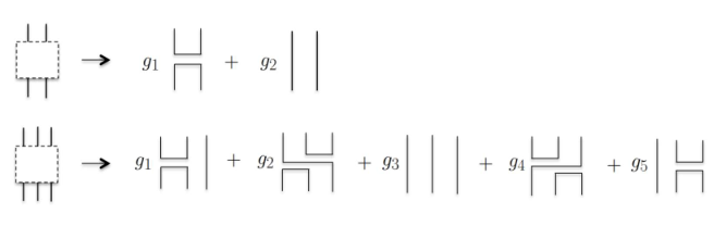
The Renyi entropy can thus be expressed as a linear combination of terms, each of which is a product of braid data and a union of Wilson loops that is a function only of the number of quasi-particles and choice of $R_{\mathcal{B}}$. We can write suggestively

$$\text{Tr}\,(\rho^{n})=\sum_{i_{1},\ldots,i_{n},j_{1},\ldots,j_{n}}\prod^{n}_{k=1}g_{i_{k}}\bar{g}_{j_{k}}\bigoplus_{\mathcal{A}}\langle Y_{i_{k}\bar{j}_{k}}\rangle,\,\,\,$$

(2.8)

where $Y_{i_{k}\bar{j}_{k}}\equiv\left(\mathcal{D}_{i}\bigoplus_{\mathcal{B}}\mathcal{D}_{6-j}\right)$ and $\langle Y_{i_{k}\bar{j}_{k}}\rangle$ denotes the Chern-Simons VEV which is obtained after identifying the open ends of $Y_{i_{k}\bar{j}_{k}}$. In this form, we see that the braid data is contained in the factors of $g_{m}$ and its conjugate whereas the dependence on $R_{\mathcal{B}}$ is expressed through the $Y_{i\bar{j}}$’s.

The coefficients $g_{i}$ are functions of the braid word. In the 2-strand case, it is simple to derive them from the skein relations. If we adopt $R_{\mathcal{B}}$ to be the entire set of quasi-particles or holes, then the density matrix is represented by the concatenation of the braid words and is always equivalent to the trivial braid. We can use this fact to obtain useful constraints for the coefficients $g_{i}$ which are ‘universal’ in the sense of being independent of the choice of $R_{\mathcal{B}}$. In the following, we work in the context of $SU(2)$ Chern-Simons theory where the skein relations is depicted in Fig. 7.

First, let us consider the two-strand case, where as depicted in Fig. 6, we merely have two coefficients $g_{1},g_{2}$. The braid is defined solely by an integer counting the number of over/under-crossings. Taking $R_{\mathcal{B}}=\{\alpha_{1},\alpha_{2}\}$, we display the various $Y_{i\bar{j}}$ in Fig. 8. Since from braid concatenation, it is clear that $\mathcal{L}_{1}$ is an unbraided 2-strand, we obtain the coefficients to satisfy

$$|g_{2}|^{2}=1,\qquad h_{0}|g_{1}|^{2}+g_{2}\bar{g}_{1}+\bar{g}_{2}g_{1}=0.$$

(2.9)

where $h_{0}=-A^{2}-A^{-2}$. In this case, we can invoke the skein relation and the form of the general braid word which is just $\sigma^{\beta},\beta\in\mathbb{Z}$ to compute $g_{1,2}=g_{1,2}(A)$ easily. We find them to be

$$g_{2}=A^{\beta},\qquad g_{1}=\frac{1}{h_{0}}\left(-A^{\beta}+(-A^{-3})^{\beta}\right)$$

(2.10)

which indeed satisfy (2.9). To derive this relation, we note that by the skein relation, every crossing yields two different arc diagrams and the only combination to obtain two unbraided lines arises from taking the first arc diagram for every crossing and thus we have a factor of $g_{2}=A^{\beta}$. For every $n$ factor of the second arc diagram, we have an additional factor of $n-1$ unknots together with a factor of $A^{-1}$. As the order does not matter, we can use a binomial expansion to keep track of the terms and thus obtain

$$g_{1}=\frac{1}{h_{0}}A^{\beta}\sum_{i=1}^{n}{}^{n}C_{i}\left(\frac{A^{-1}h_{0}}{A}\right)^{i}=\frac{1}{h_{0}}A^{\beta}\left[(1+\frac{A^{-1}h_{0}}{A})^{\beta}-1\right]=\frac{1}{h_{0}}(-A^{\beta}+(-A^{-3})^{\beta})$$

(2.11)

As another example, let us consider the 3-strand braid where we now have five coefficients $g_{i},1\leq i\leq 5$ as mentioned previously, with the various possible $Y_{i\bar{j}}$ sketched in Fig. 9. Again purposefully picking $R_{\mathcal{B}}$ to be the entire set of quasi-particles and asserting that the sum is an unbraided 3-strand, we find the constraints to read $|g_{3}|^{2}=1$ and

	$\displaystyle g_{2}\bar{g}_{1}+g_{1}\bar{g}_{2}+g_{3}\bar{g}_{1}+g_{1}\bar{g}_{3}+h_{0}(|g_{2}|^{2}+|g_{1}|^{2})$	$\displaystyle=$	$\displaystyle 0,$		(2.12)
	$\displaystyle g_{4}\bar{g}_{5}+g_{5}\bar{g}_{4}+g_{3}\bar{g}_{5}+g_{5}\bar{g}_{3}+h_{0}(|g_{4}|^{2}+|g_{5}|^{2})$	$\displaystyle=$	$\displaystyle 0,$		(2.13)
	$\displaystyle g_{3}\bar{g}_{2}+g_{4}\bar{g}_{2}+g_{5}\bar{g}_{1}+g_{4}g_{3}+h_{0}(g_{4}\bar{g}_{1}+g_{5}\bar{g}_{2})$	$\displaystyle=$	$\displaystyle 0,$		(2.14)
	$\displaystyle g_{1}\bar{g}_{5}+g_{2}\bar{g}_{4}+g_{2}\bar{g}_{3}+g_{3}\bar{g}_{4}+h_{0}(g_{1}\bar{g}_{4}+g_{2}\bar{g}_{5})$	$\displaystyle=$	$\displaystyle 0.$		(2.15)

Finally, let us briefly comment on a plausible CFT interpretation of $\langle Y_{i\bar{j}}\rangle$. In the simple case of the 2-strand braid. Taking the trace of $Y_{i\bar{j}}$, we end up with the two-by-two matrix

$$\langle Y_{i\bar{j}}\rangle=\left(\begin{array}[]{cc}Z\left(\bigcirc\cup\bigcirc\right)&Z\left(\bigcirc\right)\\ Z\left(\bigcirc\right)&Z\left(\bigcirc\cup\bigcirc\right)\end{array}\right)$$

(2.16)

Further, we can express it more suggestively as $\langle Y_{i\bar{j}}\rangle=\langle\phi_{i}|\phi_{j}\rangle$ with the inner product isomorphic to joining the punctures in region $R_{\mathcal{B}}$. Then upon orthonormalization of the matrix $\langle Y_{i\bar{j}}\rangle$, it was pointed out in [5] that the orthonormal states can be identified as the conformal blocks associated with the trivial and adjoint representation that appear in the fusion of the fundamental and anti-fundamental states, so (2.16) is essentially the fusion matrix of the CFT that lives on the boundary of the original 3-ball. It would be interesting to furnish a similar interpretation for a general $m$-strand braid and with other choices of $R_{\mathcal{B}}$.

First, let us consider a single Wilson line connecting two punctures on the sphere. Let $\mathcal{R}_{B}$ denote the region being traced out when we compute the entanglement entropies, as sketched in Fig. 10.

We find that the entanglement entropy depends on the choice of $\mathcal{R}_{B}$ as follows.

$$S_{EE}=\begin{cases}\text{Log}\,S_{j0},&R_{\mathcal{B}}=\{\bar{\alpha}\}\cr\text{Log}\,S_{00},&R_{\mathcal{B}}=\{0\}\\ \end{cases}$$

(3.1)

where $j$ denotes the representation (spin) of the Wilson line. We performed this computation by filling up the interior of $S^{2}$ to obtain a 3-ball and then gluing the appropriate discs following the surgery procedure that implements $\text{Tr}(\rho^{n})$. When $R_{\mathcal{B}}=\{\bar{\alpha}\}$, the auxiliary link $\mathcal{L}_{n}$ is the unknot independent of $n$. This implies $S_{EE}=S^{(n)}_{R}=\text{Log}\,S_{0\frac{1}{2}}$. When $R_{\mathcal{B}}=\{0\}$, $\mathcal{L}_{n}$ is the split union of $n$ unknots which yields

$$S^{(n)}_{R}=\frac{1}{1-n}\text{Log}\left((2\cos(\frac{\pi}{k+2}))^{n-1}/S_{0\frac{1}{2}}\right)=\text{Log}\left(\sqrt{\frac{2}{k+2}}\sin(\frac{\pi}{k+2})\right)=\text{Log}(S_{00})$$

(3.2)

where we observe that $S_{00}$ is the Chern-Simons partition function on $S^{3}$ (without insertion of any Wilson loops).

This result holds for other TQFTs, with $S_{j0}$ and $S_{00}$ to be replaced by the partition functions of the theory with and without an unknotted Wilson loop respectively. Clearly, in the case where $R_{\mathcal{B}}=\{\alpha,\bar{\alpha}\}\,\,\text{or}\,\,\{0\}$, the entanglement measures are insensitive to the Wilson line which intuitively does not ‘entangle’ the degrees of freedom living on both regions.

We now consider a 2-strand braid connecting two pairs of quasi-particles. A generic braid word is of the form $\sigma_{1}^{m},m\in\mathbb{Z}$. For example, when $m=\pm 2$, this yields the Hopf link. It turns out that all choices of $R_{\mathcal{B}}$ give rise to Renyi and entanglement entropies which do not distinguish the braided pair with the unbraided one, apart from the cases of $R_{\mathcal{B}}=\{\alpha_{1},\bar{\alpha}_{1}\}$ or $R_{\mathcal{B}}=\{\alpha_{2},\bar{\alpha}_{2}\}$.

In the following, for definiteness we will perform calculations in $SU(2)$ Chern-Simons theory with the braided Wilson lines in the fundamental. As noted earlier, the writhe number of the link $\mathcal{L}_{n}$ is always zero. We compute the Kauffman bracket polynomial in variable $A$ which is equivalent to the Jones polynomial (say in $t$) since the writhe number is zero⁵⁵ 5 We recall some basic definitions slightly more formally. The Kauffman bracket is a function which sends link diagrams to Laurent polynomials with integer coeffcients, so it maps the diagram $D$ to $\langle D\rangle\in\mathbb{Z}[A^{-1},A]$. It is related to the Jones polyomial of the same link $L$ by $V_{Jones}(L)=\left((-A)^{-3w(D)}\langle D\rangle\right)_{\sqrt{t}=A^{-2}}\in\mathbb{Z}[t^{-1/2},t^{1/2}]$ with $D$ being some oriented link diagram and$w(D)$ its writhe number. For the auxiliary link, we saw earlier that it is fully amphichiral and has always vanishing writhe number, so the bracket of such a link is the same as its Jones polynomial. We also take all knots and links in this paper to be in the standard framing., with

$$A=ie^{-\frac{i\pi}{2(k+2)}}=t^{-1/4}.$$

(3.3)

We made this identification by comparing (3.3) with the Chern-Simons VEV for the unknot and the split union of 2 unknots as follows. In Chern-Simons theory, the partition functions for these two Wilson loops read $Z(S^{3};\bigcirc)=S_{0\frac{1}{2}},Z(S^{3};\bigcirc\cup\bigcirc)=S^{2}_{0\frac{1}{2}}/S_{00}$ and thus their ratio reads $S_{0\frac{1}{2}}/S_{00}=2\cos\frac{\pi}{k+2}$ which is consistent with the skein relations for the Jones or Kauffman bracket polynomial if we adopt (3.3). Traces of the density matrix and its powers are equivalent to the partition function of Chern-Simons theory with the auxiliary link in $S^{3}$. In the following, we shall compute the entanglement measures for the case where $\mathcal{R}_{B}=\{\alpha_{2},\bar{\alpha}_{2}\}$. This essentially reduces to computing the Jones polynomial for the auxiliary link.

In the following we consider the case of the connected sum of two Hopf links which has the following 3-strand braid presentation as shown in Figure 17.

We find that if we choose the region $R_{B}=\{\bar{\alpha}_{3},\alpha_{2},\alpha_{3}\}$ then the Renyi entropy distinguishes it with the disjoint union of an unknot and a Hopf link or that of three unknots. We begin with the auxiliary link of which diagram is shown below in Fig. 18. This turns out to be a $(2M+1)$-component link, as depicted in Fig. 18.⁷⁷ 7 In this section, we use the index $M$ to denote the power index of the density matrix and its auxiliary link $\mathcal{L}_{M}$ for notational convenience as we choose to use the symbol $n$ as a dummy index.

We find the following skein relations in Fig.19 useful for resolving the crossings on the ‘humps’ (see Fig. 18). This reduces the link diagram eventually to the one shown on the LHS of Fig. 20.

We note that in Fig. 20, the various parameters are defined as

	$\displaystyle x=-A^{4}-\bar{A}^{4},\,\,\,\alpha=|1-A^{4}|^{2},\,\,\,y=-A^{6}-\bar{A}^{6},\,\,\,h_{0}=-A^{2}-\bar{A}^{2},\,\,\,r=\alpha/x^{2},$		(3.19)
	$\displaystyle H_{k}=|1-A^{4}|^{2k+2},\,\,\,g_{k}=yx^{2k}\left(\frac{r^{k+1}-1}{r-1}\right),\,\,\,\mathcal{P}_{k}=h_{0}H_{k}+g_{k},$		(3.20)
	$\displaystyle\mathcal{B}_{kl}=x^{2}\left(g_{k}H_{l}+g_{l}H_{k}\right)+h_{0}\left(g_{k}g_{l}+x^{2}H_{k}H_{l}\right).$		(3.21)

After some algebra, we obtain the Chern-Simons VEV to read

	$\displaystyle\langle\mathcal{L}_{M}\rangle$	$\displaystyle=$	$\displaystyle\sum_{l=1}^{M-4}\sum_{r=1}^{M-3-l}\mathcal{B}_{lr}\sum^{M-3-l-r}_{k=0}\left(\begin{array}[]{c}M-3-l-r\\ k\end{array}\right)(yh_{0})^{M-3-l-r-k}(\alpha^{k}\mathcal{P}_{k})y^{2}\alpha^{l+r}$
		$\displaystyle+$	$\displaystyle y\alpha^{M-2}\sum^{M-2}_{l=0}\mathcal{B}_{l,M-2-l}+2\sum^{M-3}_{l=1}\alpha^{l}\mathcal{B}_{l0}\sum^{M-3-l}_{k=0}\left(\begin{array}[]{c}M-3-l\\ k\end{array}\right)(yh_{0})^{M-3-l-k}\alpha^{k}\mathcal{P}_{k}y^{2}$
		$\displaystyle+$	$\displaystyle y^{2}\mathcal{B}_{00}\sum^{M-3}_{k=0}\left(\begin{array}[]{c}M-3\\ k\end{array}\right)(yh_{0})^{M-3-k}(\alpha^{k}\mathcal{P}_{k})+h_{0}\mathcal{P}_{M-1}\alpha^{M-1}$

where $\alpha=|1-A^{4}|^{2}$. As a consistency check, for every term that appears in (3.3), the powers of $y$ and $\alpha$ should sum up to $M-1$. We note that $\mathcal{P}_{k}\neq\mu^{k}$ for some $\mu=\mu(A)$, but it can be expressed as

	$\displaystyle\mathcal{P}_{m}$	$\displaystyle=$	$\displaystyle h_{0}H_{m}+g_{m}$		(3.31)
		$\displaystyle=$	$\displaystyle h_{0}|1-A^{4}|^{2}(|1-A^{4}|^{2})^{m}+\frac{yr}{r-1}(x^{2}r)^{m}+\frac{y}{1-r}(x^{2})^{m}$		(3.32)
		$\displaystyle\equiv$	$\displaystyle\sum^{2}_{i=1}C_{i}p^{m}_{i}$		(3.33)

where

$$C_{1}\equiv h_{0}\alpha+\frac{yr}{r-1},\,\,C_{2}\equiv\frac{y}{1-r},\,\,p_{1}\equiv\alpha,\,\,p_{2}\equiv x^{2}.$$

Substituting (3.33) into (3.3), we can perform the sum over the dummy index $k$ in each term to obtain

	$\displaystyle\langle\mathcal{L}_{n}\rangle$	$\displaystyle=$	$\displaystyle\sum^{2}_{i=1}C_{i}\sum^{M-4}_{l}\sum^{M-3-l}_{r=1}\mathcal{B}_{lr}(yh_{0}+\alpha p_{i})^{M-3-l-r}y^{2}\alpha^{l+r}+h_{0}\mathcal{P}_{M-1}\alpha^{M-1}$		(3.34)
		$\displaystyle+$	$\displaystyle\sum^{2}_{i=1}C_{i}y^{2}\mathcal{B}_{00}(yh_{0}+\alpha p_{i})^{M-3}+y\alpha^{M-2}\sum^{M-2}_{l=0}\mathcal{B}_{l,M-2-l}$		(3.35)
		$\displaystyle+$	$\displaystyle 2\sum^{2}_{i=1}C_{i}\sum^{M-3}_{l=1}\alpha^{l}\mathcal{B}_{l0}(yh_{0}+\alpha p_{i})^{M-3-l}y^{2}.$		(3.36)

We note that after some simplification, $\mathcal{B}_{kl}$ can be written in the form

$$\mathcal{B}_{kl}=\sum^{2}_{m,n=1}b_{mn}p^{k}_{m}p^{l}_{n}$$

(3.37)

where

$$b_{11}=2\alpha^{2}C_{2}+h_{0}(C^{2}_{2}r^{2}+x^{2}\alpha^{2}),b_{12}=b_{21}=-h_{0}rC^{2}_{2}-x^{2}\alpha C_{2},b_{22}=h_{0}C^{2}_{2}.$$

Substituting (3.37) into (3.36), we obtain

	$\displaystyle\langle\mathcal{L}_{M}\rangle$	$\displaystyle=$	$\displaystyle y^{2}\sum^{2}_{i,k,l=1}C_{i}\sum^{M-4}_{l=1}\sum^{M-3-l}_{r=1}b_{kl}p^{l}_{m}p^{r}_{n}(yh_{0}+\alpha p_{i})^{M-3-l-r}\alpha^{l+r}+h_{0}\mathcal{P}_{M-1}\alpha^{M-1}$		(3.38)
		$\displaystyle+$	$\displaystyle\sum^{2}_{i=1}C_{i}y^{2}\mathcal{B}_{00}(yh_{0}+\alpha p_{i})^{M-3}+y\alpha^{M-2}\sum^{M-2}_{l=0}\sum^{2}_{m,n=1}b_{mn}p^{l}_{m}p^{M-2-l}_{n}$		(3.39)
		$\displaystyle+$	$\displaystyle 2\sum^{2}_{i=1}C_{i}\sum^{M-3}_{l=1}\sum^{2}_{m,n=1}\alpha^{l}b_{mn}p^{l}_{m}(yh_{0}+\alpha p_{i})^{M-3-l}y^{2}$		(3.40)
		$\displaystyle\equiv$	$\displaystyle y^{2}\sum^{2}_{i,m,n=1}C_{i}b_{mn}\sum^{M-4}_{l=1}\sum^{M-3-l}_{r=1}p^{l}_{m}p^{r}_{n}h^{M-3-l-r}_{i}\alpha^{l+r}$		(3.41)
		$\displaystyle+$	$\displaystyle y^{2}\mathcal{B}_{00}\sum^{2}_{i=1}C_{i}h^{M-3}_{i}+y\alpha^{M-2}\sum^{2}_{m,n=1}\sum^{M-2}_{l=0}p^{l}_{m}p^{M-2-l}_{n}$		(3.42)
		$\displaystyle+$	$\displaystyle 2y^{2}\sum^{2}_{i,m,n=1}b_{mn}C_{i}\sum^{M-3}_{l=1}\alpha^{l}p^{l}_{m}h^{M-3-l}_{i}+h_{0}\mathcal{P}_{M-1}\alpha^{M-1}.$		(3.43)

where we define $h_{i}=yh_{0}+\alpha p_{i}$. In this form, it is evident that we can express the Jones polynomial explicitly as a function of $M$. We now perform the sum over the indices $l$ and $r$ in each term in (3.43). The various geometric sums read

$$\sum^{M-3}_{l=1}\alpha^{l}p^{l}_{m}\frac{h^{M-3}_{i}}{h^{l}_{i}}=h^{M-3}_{i}\sum^{M-3}_{l=1}\left[\frac{\alpha p_{m}}{h_{i}}\right]^{l}\equiv h^{M-3}_{i}\sum^{M-3}_{l=1}U^{l}_{mi}=h^{M-3}_{i}U_{mi}\frac{(U^{M-3}_{mi}-1)}{U_{mi}-1},$$

(3.44)

$$\sum^{M-2}_{l=0}\left[\frac{p_{m}}{p_{n}}\right]^{l}p^{M-2}_{n}\equiv p^{M-2}_{n}\sum^{M-2}_{l=0}V^{l}_{mn}=p^{M-2}_{n}\frac{V^{M-1}_{mn}-1}{V_{mn}-1}$$

(3.45)

	$\displaystyle\sum^{M-4}_{l=1}p^{l}_{m}h^{M-3-l}_{i}\alpha^{l}\sum^{M-3-l}_{r=1}\left[\frac{p_{n}\alpha}{h_{i}}\right]^{r}$	$\displaystyle=$	$\displaystyle h^{M-3}_{i}\sum^{M-4}_{l=1}\left[\frac{p_{m}\alpha}{h_{i}}\right]^{l}\sum^{M-3-l}_{r=1}U^{r}_{ni}$		(3.46)
		$\displaystyle=$	$\displaystyle h^{M-3}_{i}\sum^{M-4}_{l=1}\left[\frac{p_{m}\alpha}{h_{i}}\right]^{l}\frac{U_{ni}(U^{M-3-l}_{ni}-1)}{U_{ni}-1}$		(3.47)
		$\displaystyle\equiv$	$\displaystyle h^{M-3}_{i}\left[\frac{U^{M-2}_{ni}}{U_{ni}-1}\frac{V_{mn}(V^{M-4}_{mn}-1)}{(V_{mn}-1)}-\frac{U_{ni}}{U_{ni}-1}\frac{U_{mi}(U^{M-4}_{mi}-1)}{(U_{mi}-1)}\right]$

where

$$U_{mi}\equiv\frac{\alpha p_{m}}{h_{i}},\,\,V_{mn}=\frac{p_{m}}{p_{n}}.$$

Finally, assembling all the terms together, the Jones polynomial of the auxiliary link reads

	$\displaystyle\langle\mathcal{L}_{M}\rangle$	$\displaystyle=$	$\displaystyle y^{2}\sum^{2}_{i,m,n=1}C_{i}b_{mn}h^{M-3}_{i}\left[\frac{U^{M-2}_{ni}}{U_{ni}-1}\frac{V_{mn}(V^{M-4}_{mn}-1)}{(V_{mn}-1)}-\frac{U_{ni}}{U_{ni}-1}\frac{U_{mi}(U^{M-4}_{mi}-1)}{(U_{mi}-1)}\right]$		(3.49)
		$\displaystyle+$	$\displaystyle y^{2}\mathcal{B}_{00}\sum^{2}_{i=1}C_{i}h^{M-3}_{i}+y\alpha^{M-2}\sum^{2}_{m,n=1}b_{mn}p^{M-2}_{n}\frac{V^{M-1}_{mn}-1}{V_{mn}-1}$		(3.50)
		$\displaystyle+$	$\displaystyle 2y^{2}\sum^{2}_{i,m,n=1}b_{mn}C_{i}h^{M-3}_{i}U_{mi}\frac{(U^{M-3}_{mi}-1)}{U_{mi}-1}+h_{0}\sum^{2}_{i=1}C_{i}(\alpha p_{i})^{M-1}.$		(3.51)

This expression is manifestly valid for $M>4$ which we use to derive the Jones polynomial. However, as a function in $M$, we find that it naturally extends to all lower values. To verify this, we list the polynomial $\langle\mathcal{L}_{M}\rangle$ for each lower value of $M$ below.

	$\displaystyle\langle\mathcal{L}_{4}\rangle$	$\displaystyle=$	$\displaystyle h_{0}\mathcal{P}_{3}\alpha^{3}+y^{2}\mathcal{B}_{00}\sum_{k=0}^{1}(yh_{0})^{1-k}\alpha^{k}\mathcal{P}_{k}+y\alpha^{2}\sum_{l=0}^{2}\mathcal{B}_{l,2-l}+2y^{2}\alpha\mathcal{B}_{10}\mathcal{P}_{0}y^{2},$		(3.52)
	$\displaystyle\langle\mathcal{L}_{3}\rangle$	$\displaystyle=$	$\displaystyle 2y\alpha\mathcal{B}_{10}+h_{0}\mathcal{P}_{2}\alpha^{2}+y^{2}\mathcal{P}_{0}\mathcal{B}_{00},$		(3.53)
	$\displaystyle\langle\mathcal{L}_{2}\rangle$	$\displaystyle=$	$\displaystyle y\mathcal{B}_{00}+h_{0}\mathcal{P}_{1}\alpha,\,\,\,\langle\mathcal{L}_{1}\rangle=h^{2}_{0}$		(3.54)

For $M=1$, only the term $h_{0}\sum_{i}C_{i}(\alpha p_{i})^{M-1}=h^{2}_{0}$ survives and this yields the Jones polynomial of the split union of three unknots which is expected of $\text{Tr}\rho$. We check that we can indeed obtain (3.52)-(3.54) from (3.51) which can be expressed in a form manifestly appropriate for all $M\geq 1$ as follows.

References

- [1] W. Donnelly, “Entanglement entropy and nonabelian gauge symmetry,” Class. Quant. Grav. 31, no. 21, 214003 (2014) doi:10.1088/0264-9381/31/21/214003 [arXiv:1406.7304 [hep-th]].
- [2] S. Ryu and T. Takayanagi, “Holographic derivation of entanglement entropy from AdS/CFT,” Phys. Rev. Lett. 96, 181602 (2006) doi:10.1103/PhysRevLett.96.181602 [hep-th/0603001].
- [3] A. Kitaev and J. Preskill, “Topological entanglement entropy,” Phys. Rev. Lett. 96, 110404 (2006) doi:10.1103/PhysRevLett.96.110404 [hep-th/0510092].
- [4] M. Levin and X. G. Wen, “Detecting Topological Order in a Ground State Wave Function,” Phys. Rev. Lett. 96, 110405 (2006). doi:10.1103/PhysRevLett.96.110405
- [5] S. Dong, E. Fradkin, R. G. Leigh and S. Nowling, “Topological Entanglement Entropy in Chern-Simons Theories and Quantum Hall Fluids,” JHEP 0805, 016 (2008) doi:10.1088/1126-6708/2008/05/016 [arXiv:0802.3231 [hep-th]].
- [6] X. Wen, S. Matsuura and S. Ryu, “Edge theory approach to topological entanglement entropy, mutual information and entanglement negativity in Chern-Simons theories,” Phys. Rev. B 93, no. 24, 245140 (2016) doi:10.1103/PhysRevB.93.245140 [arXiv:1603.08534 [cond-mat.mes-hall]].
- [7] D. Das and S. Datta, “Universal features of left-right entanglement entropy,” Phys. Rev. Lett. 115, no. 13, 131602 (2015) doi:10.1103/PhysRevLett.115.131602 [arXiv:1504.02475 [hep-th]].
- [8] L.H. Kauffman and E.Mehrotra, “Topological Aspects of Quantum Entanglement,” [arXiv:1611.08047 [math.GT]]
- [9] G. Salton, B. Swingle and M. Walter, “Entanglement from Topology in Chern-Simons Theory,” Phys. Rev. D 95, no. 10, 105007 (2017) doi:10.1103/PhysRevD.95.105007 [arXiv:1611.01516 [quant-ph]].
- [10] V. Balasubramanian, J. R. Fliss, R. G. Leigh and O. Parrikar, “Multi-Boundary Entanglement in Chern-Simons Theory and Link Invariants,” arXiv:1611.05460 [hep-th].
- [11] E. Witten, “Quantum Field Theory and the Jones Polynomial,” Commun. Math. Phys. 121, 351 (1989). doi:10.1007/BF01217730
- [12] C. de C. Chamon, D. E. Freed, S. A. Kivelson, S. L. Sondhi, and X. G. Wen, “Two point-contact interferometer for quantum Hall systems,” Phys. Rev. B 55, 2331 (1997) [arXiv:cond-mat/9607195]
- [13] S. Gukov, “Three-dimensional quantum gravity, Chern-Simons theory, and the A polynomial,” Commun. Math. Phys. 255, 577 (2005) doi:10.1007/s00220-005-1312-y [hep-th/0306165].
- [14] S. Carlip, “Exact Quantum Scattering in (2+1)-Dimensional Gravity,” Nucl. Phys. B 324, 106 (1989). doi:10.1016/0550-3213(89)90183-1
- [15] S. Jackson, L. McGough and H. Verlinde, “Conformal Bootstrap, Universality and Gravitational Scattering,” Nucl. Phys. B 901, 382 (2015) doi:10.1016/j.nuclphysb.2015.10.013 [arXiv:1412.5205 [hep-th]].
- [16] W.B.R. Lickorish, “An Introduction to Knot Theory,” Graduate Texts in Mathematics, Springer-Verlag, New York, 1997.
- [17] J.S. Birman, “Braids, Links, and Mapping Class Groups,” Annals of Math Studies 82, Princeton University Press, USA, 1975.
- [18] R.A. Landvoy, “The Jones polynomial of pretzel knots and links,” Topology and its applications 83, Issue 2, 135-147 (1998). doi:10.1016/S0166-8641(97)00100-4
- [19] L. Rozansky and H. Saleur, “Reidemeister torsion, the Alexander polynomial and U(1,1) Chern-Simons Theory,” J. Geom. Phys. 13, 105 (1994) doi:10.1016/0393-0440(94)90022-1 [hep-th/9209073].
- [20] M. Aganagic and S. Shakirov, “Refined Chern-Simons Theory and Knot Homology,” Proc. Symp. Pure Math. 85, 3 (2012) doi:10.1090/pspum/085/1372 [arXiv:1202.2489 [hep-th]].
- [21] H.S. Tan, Work in preparation.
- [22] D. Bar-Natan, S. Morrison et al., “The Knot Atlas,” http://katlas.org