An Integro-Differential Structure for Dirac Distributions

It is indisputable that differential algebra Ritt (1966); Kolchin (1973), differential Galois theory Put, Singer (2003) as well as various other approaches of Symbolic Analysis have made outstanding contributions to the theory of differential equations Seiler (1997). From their particular algebraic-algorithmic vantage points, they provide powerful tools for describing and analyzing the structure of solutions. Interestingly, the theory of distributions—in modern analysis the hard bedrock supporting the theory of linear (ordinary and partial) differential equations—has received comparably little attention in Symbolic Analysis.

One reason for this is perhaps that the standard approach to distributions seems to be inherently topological in nature; even the very definition of distributions involves the continuous dual of certain carefully chosen function spaces Duistermaat, Kolk (2010). Of course, such an objection begs the question: Namely, how much algebraic structure can one extract from the Algebra-Analysis mixture at first encountered? Even differential algebra was in the same situation before basic notions such as differential rings were introduced.

Based on the results of the present paper, we think the main obstacle to an algebraic treatment of distributions is the widespread limitation of differential algebra to structures having only derivations (differential rings / fields / algebras / modules). In a setting thus limited, one can say little more than the following: “A distribution like $\delta_{a}$ has arbitrary formal derivatives $\delta_{a}^{\prime},\delta_{a}^{\prime\prime},\dots$”. In effect, one treats $\delta_{a}$ as a differential indeterminate. But the characteristic feature of the Dirac distribution $\delta_{a}$ is of course that it effects an evaluation at $a$ when it “appears under the integral”. For making this central idea precise (in algebraic terms), one has to take recourse to the theory of Rota-Baxter algebras Guo (2012). By the same token, one must also provide an algebraic treatment of evaluation; both of these are linked in the structure of integro-differential algebras Rosenkranz Regensburger (2008) by a crucial relation (3).

Once integration enters the stage, it is clear that we should also consider piecewise functions since the latter may be built up from the Heaviside function $H_{a}(x)=H(x-a)$, which is in turn the integral of the Dirac delta distribution $\delta_{a}$. In fact, it is natural to start with the theory of piecewise (smooth or continuous) functions since these may usefully be endowed with a Rota-Baxter operator without involving distributions. One might even be tempted to build up distributions via this route, simply adding a derivation that maps $H_{a}$ to the Dirac distribution $\delta_{a}$. As we shall see subsequently (Remark 13), our actual development must follow a slightly different route, though we shall indeed treat piecewise functions before introducing Dirac distributions.

Assuming one can extract some “algebraic substance” from the theory of distributions, what does it achieve? In particular, does it allow any symbolic computation for practically important applications? We think the answer is yes, as we would like to demonstrate here: While the primary purpose of this paper is to lay out the foundations, we do include an application section to sketch one domain where our algebraic approach to distributions can be employed—boundary problems for linear ordinary differential equations (LODE). Here distributions come into their own: As we shall see in detail, one may actually distinguish three different (though related) roles for the algebraic Heaviside functions and Dirac distributions: (1) The Green’s function of a regular boundary problem is naturally a piecewise function (or even a proper distribution in the case of ill-posed boundary problems). (2) It can be shown to satisfy a differential equation with the Dirac distribution on its right-hand side. (3) The Green’s operator may act on functions which are only piecewise smooth.

Of course this does not exhaust the possible scope of applications. Eventually, computer algebra systems like Maple^TM and Mathematica^® should be able to treat distributions and piecewise functions much like any other “functional” terms. They should provide support for all crucial operations on these objects, including many that we cannot address here (e.g. convolution, Fourier/Laplace transforms, composition). For practical applications, one often needs to be able to use piecewise functions and distributions at suitable places in algebraic and differential equations to be solved or simplified. We hope our approach will provide a convenient starting point for further development in this direction.

Structure of the paper. In detail, we will develop the subject matter as follows. After completing this Introduction by explaining some crucial notation, we briefly review the theory of differential Rota-Baxter algebras and modules, which form the basic algebraic framework for the rest of the paper (Section 2). In the next section we build up the algebra of piecewise functions and show that is a Rota-Baxter extension of the ground algebra (Proposition 4), generalizing the familiar setting of piecewise smooth or piecewise analytic functions (Examples 7 and 8). Then distributions are introduced as a differential Rota-Baxter module (Section 4), following an independent route but such that the piecewise functions reappear as a Rota-Baxter subalgebra (Theorem 12). In fact, we shall see that the distributions even form an integro-differential module (Proposition 15), that they can be characterized by a natural universal property (Proposition 17), and that they inherit the shift structure from the ground algebra (Theorem 18). We end the section by exhibiting the filtration structure of the integro-differential module of distributions. The topic of the next section is a—rather modest—species of bivariate distributions (Section 5), though large enough to cater for the applications of the next section. Just as the univariate distribution module contains the Rota-Baxter subalgebra of piecewise functions, the bivariate version contains the bivariate piecewise functions as a subalgebra relative to both Rota-Baxter structures (Proposition 23). However, the main result of this section is that the bivariate distribution module is a differential Rota-Baxter module with respect to both differential Rota-Baxter structures, containing isomorphic copies of both univariate distribution modules plus “diagonal” distributions (Theorem 24). Equipped with these tools, we turn to the aforementioned applications in the theory of LODE boundary problems (Section 6). Our first goal is to generalize the algorithm extracting Green’s functions from Green’s operators given in Rosenkranz, Serwa (2015) to bivariate distributions over ordinary shifted integro-differential algebras (Theorem 26). Next we show that such a Green’s function also satisfies an algebraic version of the well-known distributional differential equation with $\delta(x-\xi)$ on the right-hand side (Theorem 29). Finally, we confirm that the corresponding Green’s operator of an arbitrary well-posed boundary problem may actually be applied to piecewise functions (Proposition 30). We conclude with some thoughts about future developments.

Notation. With the exception of the ring of integro-differential operators (to be introduced in Section 2), all rings and algebras in this paper are assumed to be commutative and—unless stated otherwise—also unitary. Algebras are over a ground ring $K$ that will usually be a field (in fact an ordered field for most of the time). The set of nonzero elements of $K$ is denoted by $K^{\times}$. We write $\mathrm{Aut}_{K}(\mathcal{F})$ for the group of $K$-algebra automorphisms of an algebra $\mathcal{F}$. By a character of $\mathcal{F}$ we mean an algebra homomorphism $\mathcal{F}\to K$. If $P$ and $Q$ are any linear operators on $\mathcal{F}$, their commutator is denoted by $[P,Q]:=PQ-QP$. If $S$ is a semigroup, we write $\mathcal{F}[S]$ for the semigroup algebra of $S$ over $\mathcal{F}$, by which we mean the monoid algebra (Lang, 2002, p. 104) of the unitarization $S\uplus\{1\}$.

If $(\mathcal{F},\partial)$ is a differential algebra, we write as usual $f^{\prime}:=\partial f$ and $f^{(k)}=\partial^{k}f$ for the derivatives of an element $f\in\mathcal{F}$. For a set of differential indeterminates $X$, the algebra of differential polynomials $\mathcal{F}\{X\}$ is the free object in the category of differential $\mathcal{F}$-algebras. Similarly, the $\mathcal{F}$-submodule $\mathcal{F}\{X\}_{1}$ consisting of affine differential polynomials, i.e. those having total degree at most $1$, is the free object in the category of differential $\mathcal{F}$-modules.

Since in Section 3 we will be dealing with $K$-algebras where $(K,<)$ is an ordered field (hence of characteristic zero), it is useful to introduce some notation for ordered fields. We denote the minimum and maximum of two elements $a,b\in K$ by $a\sqcap b$ and $a\sqcup b$, respectively. We agree that $\sqcap,\sqcup$ have precedence over $+,-$. Furthermore, we shall write $a^{+}:=a\sqcup 0$ and $a^{-}:=a\sqcap 0$ for the positive and negative part of $a\in K$; then we have $a=a^{+}+a^{-}$ and $|a|=a^{+}-a^{-}$. We observe that both $(K,\sqcap)$ and $(K,\sqcup)$ are semigroups, which we denote by $K_{\sqcap}$ and $K_{\sqcup}$, respectively. We define the Heaviside operator $H\colon K\to K$ by

for $a\in K$. The appropriate choice of $\eta\in K$ is somewhat subtle; we will repeatedly come back to this point. From the analytic point of view, we might think of the mapping $\mathbbm{R}\to\mathbbm{R},a\mapsto H(a)$ as a (representative of an) $L^{2}$ function¹¹ 1 These remarks are purely motivational. It is important to distinguish $H(a)$ from $H_{a}$, which we shall introduce below, in Definition 2, as the actual algebraic model of the Heaviside function $x\mapsto H(x-a)$., and then the choice of $\eta\in\mathbbm{R}$ is of course immaterial. For the algebraic treatment, however, we will distinguish three more or less natural possibilities (the terminology is again motivated by the case $K=\mathbbm{R}$):

• •

  The left continuous convention uses $\eta=0$.

• •

  In contrast, the right continuous choice is to put $\eta=1$.

• •

  Finally, the symmetric setting $\eta=1/2$ is essentially the sign function in the sense that one has $\operatorname{sgn}(a)=2H(a)-1$. It is neither left nor right continuous.

In this paper, we use the left-continuous convention $\eta=0$, but we will discuss the other possibilities as we develop the corresponding algebraic structures. For convenience we shall use also $\bar{H}(x):=1-H(x)$ for the dual Heaviside operator.

Just as a differential algebra $(\mathcal{F},\partial)$ encodes the essence of derivatives, the basic algebraic structure for encoding integration is a Rota-Baxter algebra $(\mathcal{F},{\textstyle\int})$, meaning a $K$-algebra with a $K$-linear operator ${\textstyle\int}\colon\mathcal{F}\to\mathcal{F}$ satisfying the Rota-Baxter axiom

which we also call the weak Rota-Baxter axiom in view of an important generalization that we shall explain soon. At this juncture we should point out our parenthesis convention for nested Rota-Baxter operators:²² 2 Note also that here and henceforth we use operator notation for $\partial$ and ${\textstyle\int}$, as it is common in analysis. So the Leibniz rule is $\partial\,fg=f\partial g+g\partial f$ rather than $d(fg)=f\,d(g)+g\,d(f)$ when using functional notation with $d$. In the same vein, (1) would be $P(f)\,P(g)=P(f\,P(g))+P(g\,P(f))$ in functional notation with $P$. The scope of ${\textstyle\int}$ extends across all implicit products (denoted by juxtaposition), terminated by $\cdot$ as on the left-hand side of (1). While this saves a host of parentheses, one must be careful to distinguish ${\textstyle\int}f\,{\textstyle\int}g$ and ${\textstyle\int}f\cdot{\textstyle\int}g$.

It is often necessary to combine differential and Rota-Baxter structures, especially for application areas like boundary problems, but also for the algebraic theory of distributions that we are about to build up. There are two important ways of coupling the two structures. The weaker one is called a differential Rota-Baxter algebra $(\mathcal{F},\partial,{\textstyle\int})$ in Guo, Keigher (2008); by definition this is a differential algebra $(\mathcal{F},\partial)$ and a Rota-Baxter algebra $(\mathcal{F},{\textstyle\int})$ such that the Rota-Baxter operator ${\textstyle\int}$ is a section of the derivation $\partial$. Thus the differential and Rota-Baxter structures are only coupled by the so-called section axiom $\partial\circ{\textstyle\int}=1_{\mathcal{F}}$.

In many cases the coupling is stronger: We call $(\mathcal{F},{\textstyle\int},\partial)$ an integro-differential algebra if $(\mathcal{F},\partial)$ is a differential algebra and ${\textstyle\int}\colon\mathcal{F}\to\mathcal{F}$ is a $K$-linear operator satisfying the strong³³ 3 In Rosenkranz Regensburger (2008) we have called it the “differential Rota-Baxter axiom”. In the present context we prefer to avoid this terminology as it might be misconstrued as characterizing differential Rota-Baxter algebras. Rota-Baxter axiom (Rosenkranz Regensburger, 2008, Eqn. (6)), namely

This terminology stems from the fact that the weak axiom (1) is a consequence (just replace $f$ by ${\textstyle\int}f$ in the strong axiom and use the section axiom) while there are differential Rota-Baxter algebras that are not integro-differential algebras. The first such example was found by G. Regensburger, using a quotient of a polynomial ring (Rosenkranz Regensburger, 2008, Ex. 3). In fact, we shall soon encounter a natural example from analysis, namely piecewise smooth functions “interpreted in the $L^{2}$ style” (Proposition 6).

There are various equivalent characterizations of the difference between differential Rota-Baxter and integro-differential algebras (Guo, Regensburger, Rosenkranz, 2012, Thm. 2.5), for example that $\operatorname{Im}{{\textstyle\int}}\subset\mathcal{F}$ is an ideal rather than a subalgebra, or that ${\textstyle\int}$ is linear not just over $K$ but over $\operatorname{Ker}{\partial}$. One reformulation that is important here involves the so-called induced evaluation

which is a just projector onto $K$ along $\operatorname{Im}{{\textstyle\int}}$ for a general differential Rota-Baxter algebra but moreover multiplicative for an integro-differential algebra.

We call an (integro-)differential algebra ordinary if $\operatorname{Ker}{\partial}=K$. In that case, e is a linear functional for a general differential Rota-Baxter algebra and a character for an integro-differential algebra. We will usually start from an ordinary integro-differential algebra $(\mathcal{F},\partial,{\textstyle\int})$. In fact, ordinary differential Rota-Baxter algebras are automatically integro-differential (since then linearity over $K$ is actually over $\operatorname{Ker}{\partial}$).

The notion of evaluation is crucial for the algebraic theory of integration. For certain purposes (cf. Definition 3), it will thus be useful to extend it to the more general setting of a plain Rota-Baxter algebra $(\mathcal{F},{\textstyle\int})$, where an evaluation is any character $\text{{e}}\colon\mathcal{F}\to K$ with $\text{{e}}{\textstyle\int}=0$. This generalizes also the case of so-called ordinary Rota-Baxter algebras Rosenkranz, Gao, Guo (2015), defined as Rota-Baxter algebras $(\mathcal{F},{\textstyle\int})$ where ${\textstyle\int}\colon\mathcal{F}\to\mathcal{F}$ is injective and $\operatorname{Im}({\textstyle\int})\dotplus K=\mathcal{F}$; the projector e onto $K$ along $\operatorname{Im}({\textstyle\int})$ is then a distinguished evaluation. As noted in Rosenkranz, Gao, Guo (2015), each ordinary Rota-Baxter algebra corresponds to a unique integro-differential algebra $(\mathcal{F},\partial,{\textstyle\int})$ such that (3) holds; $(\mathcal{F},\partial,{\textstyle\int})$ is thus ordinary in the usual sense of $\operatorname{Ker}{\partial}=K$.

We think of the evaluation as evaluating at a certain point $o$, namely the (implicit) initialization point of the Rota-Baxter operator ${\textstyle\int}={\textstyle\int}_{\!o}^{x}$. While this is only suggestive notation, we can consider an arbitrary character $\varphi\colon\mathcal{F}\to K$ and turn the given Rota-Baxter operator ${\textstyle\int}$ into a new one ${\textstyle\int}_{\!\varphi}:=(1-\varphi){\textstyle\int}$ that we call initialized at $\varphi$. Its initialized function space $\operatorname{Im}{{\textstyle\int}_{\!\varphi}}$ is given by $\operatorname{Ker}{\varphi}$, the functions “vanishing at $\varphi$”. This may be viewed as an algebraic description of integrals ${\textstyle\int}_{\!\varphi}^{x}$ from various fixed initialization points $\varphi$ to the variable upper bound $x$. We will have a more rigid connection when we construct piecewise functions via shift maps (Definition 3), labeling the characters $\varphi=\text{{e}}_{c}$ by points $c\in K$. In this context we will often use $f(c)$ as a suggestive shorthand for $\text{{e}}_{c}(f)$, likewise ${\textstyle\int}_{\!c}$ for ${\textstyle\int}_{\!\text{{e}}_{c}}$.

Within this paper we cannot review the theory and algorithms for linear boundary problems over an ordinary integro-differential algebra $(\mathcal{F},\partial,{\textstyle\int})$; let us refer the reader to Rosenkranz Regensburger (2008). Here we just recall that, given a collection $\Phi$ of characters $\mathcal{F}\to K$, one constructs the ring of integro-differential operators $\mathcal{F}_{\Phi}[\partial,{\textstyle\int}]$ with canonical direct decomposition

as $K$-vector spaces; here $\mathcal{F}[\partial]$ is the usual ring of differential operators and $\mathcal{F}[{\textstyle\int}]$ the corresponding (nonunitary) ring of integral operators (generated over $\mathcal{F}$ by ${\textstyle\int}$) while $(\Phi)$ is the two-sided ideal generated by the character set $\Phi$. The latter may be characterized as left $\mathcal{F}$-module generated by Stieltjes conditions, defined as the right ideal $\Phi\cdot\mathcal{F}_{\Phi}[\partial,{\textstyle\int}]$. In the standard example above, these are arbitrary linear combinations of local conditions (derivative evaluations of any order) and global conditions (definite integrals with premultiplied weighting functions).

A boundary problem is a pair $(T,\mathcal{B})$ consisting of a monic differential operator $T\in\mathcal{F}[\partial]$ of order $n$ and a boundary space $\mathcal{B}\subset\mathcal{F}^{*}$ spanned by $n$ linearly independent Stieltjes conditions $\beta_{1},\dots,\beta_{n}$. We call $(T,\mathcal{B})$ regular iff $\operatorname{Ker}{T}\dotplus\mathcal{B}^{\perp}=\mathcal{F}$, where the orthogonal is defined as the admissible function space $\mathcal{B}^{\perp}:=\{f\in\mathcal{F}\mid\forall_{\beta\in\mathcal{B}}\>\beta(f)=0\}$. Regularity of $(T,\mathcal{B})$ is equivalent to the classical stipulation: There is exactly one solution $u\in\mathcal{F}$ of

for every forcing function $f\in\mathcal{F}$. Having a fundamental system $u_{1},\dots,u_{n}$ of the homogeneous system, meaning a $K$-basis of $\operatorname{Ker}{T}$, this may be checked algorithmically: The regularity of $(T,\mathcal{B})$ is equivalent to the regularity of the evaluation matrix $\beta(u)\in K^{n\times n}$ formed by evaluating each $\beta_{i}\in\mathcal{B}$ on each $u_{j}\in\operatorname{Ker}{T}$.

The Green’s operator $G$ of a regular boundary problem $(T,\mathcal{B})$ is characterized by the relations $TG=1_{\mathcal{F}}$ and $\operatorname{Im}{G}=\mathcal{B}^{\perp}$; it is the map $f\mapsto u$ for (4) and may be computed as an element of the operator ring $G\in\mathcal{F}_{\Phi}[\partial,{\textstyle\int}]$. Using the natural action of $\mathcal{F}_{\Phi}[\partial,{\textstyle\int}]$ on $\mathcal{F}$, one may check that $u:=Gf$ actually satisfies (4).

The above ring-theoretic notions (differential algebra, Rota-Baxter algebra, differential Rota-Baxter algebra, integro-differential algebra) all have natural module-theoretic analogs. For example, a differential Rota-Baxter module $(M,\eth,{\textstyle{\vbox{\hbox{$\scriptscriptstyle\diagup$}}\kern-5.13895pt}\!\int})$ over a differential Rota-Baxter algebra $(\mathcal{F},\partial,{\textstyle\int})$ consists of a derivation $\eth\colon M\to M$ in the sense that $\eth\,f\varphi=(\partial f)\,\varphi+f\,\eth\varphi$ for $f\in\mathcal{F}$ and $\varphi\in M$, and a Rota-Baxter operator ${\textstyle{\vbox{\hbox{$\scriptscriptstyle\diagup$}}\kern-5.13895pt}\!\int}\colon M\to M$ characterized by the (weak) Rota-Baxter axiom

for $f\in\mathcal{F}$ and $\varphi\in M$; confer also (Gao, Guo, Rosenkranz, 2015, Ex. 3.7(b)). It is now also clear what one means by a Rota-Baxter module. The notion of integro-differential module, however, is slightly more subtle since we must now distinguish the strong Rota-Baxter axiom (2) for coefficients and the one for module elements; we shall postpone this discussion to later when it is needed (Lemma 14). For now let us just agree to call $(M,\eth,{\textstyle{\vbox{\hbox{$\scriptscriptstyle\diagup$}}\kern-5.13895pt}\!\int})$ ordinary iff $\operatorname{Ker}{\eth}=K$.

When dealing with bivariate distributions, we shall come across algebras with two distinct differential and/or Rota-Baxter structures. In such a case we shall speak of duplex structures. For example, a duplex Rota-Baxter algebra $(\mathcal{F}_{2},\partial_{x},\partial_{\xi},{\textstyle\int}^{x},{\textstyle\int}^{\xi})$ is characterized by requiring both $(\mathcal{F}_{2},\partial_{x},{\textstyle\int}^{\xi})$ and $(\mathcal{F}_{2},\partial_{\xi},{\textstyle\int}^{x})$ to be Rota-Baxter algebras. (It should be noted that from our algebraic viewpoint $\partial_{x},\partial_{\xi}$ and ${\textstyle\int}^{x},{\textstyle\int}^{\xi}$ are just two pairs of derivations and Rota-Baxter operators that we might as well call $d,e$ and $P,Q$ should we care to.)

The passage from smooth functions $C^{\infty}(\mathbbm{R})$ to piecewise smooth functions $PC^{\infty}(\mathbbm{R})$ can be achieved by adding characteristic functions for all intervals $[a,b]\subset\mathbbm{R}$, and these can in turn be generated by the well-known Heaviside function $H(x)\in PC^{\infty}(\mathbbm{R})$ as $1_{[a,b]}(x)=H(x-a)\,H(b-x)$. We shall come back to this motivating instance (Example 7).

Our present goal is to describe the passage from a suitable integro-differential algebra $\mathcal{F}$ to its piecewise extension $\mathcal{P}\mathcal{F}$ in an abstract algebraic manner. As we have just seen, it is sufficient to adjoin algebraic Heaviside functions to $\mathcal{F}$. These can be defined in a natural way if the ground field $K$ of the given integro-differential algebra $\mathcal{F}$ is an ordered field⁴⁴ 4 Distributions are usually defined as generalizations of functions of a real variable, meaning either $\mathbbm{R}^{n}\to\mathbbm{R}$ or $\mathbbm{R}^{n}\to\mathbbm{C}$. The case of a complex variable $\mathbbm{C}^{n}\to\mathbbm{C}$ is effectively treated as $\mathbbm{R}^{2n}\to\mathbbm{C}$, ignoring the field structure of $\mathbbm{C}\cong\mathbbm{R}\times\mathbbm{R}$. Starting from an ordered field thus seems plausible.; in classical analysis this is of course $K=\mathbbm{R}$. For the algebraic construction it is sufficient to employ the semigroup algebra of $K_{\sqcup}$ over $\mathcal{F}$.

We denote the identity element of $\mathcal{P}\mathcal{F}$ by $1$ and the other generators by $H_{a}\>(a\in K)$. Then $\mathcal{P}\mathcal{F}$ can be viewed as the quotient of the polynomial ring $\mathcal{F}[H_{a}\mid a\in K]$ modulo the ideal generated by the relations $H_{a}H_{b}-H_{a\sqcup b}\>(a,b\in K)$. Moreover, linearity of the order on $K$ gives rise to the exchange law $H_{a\sqcup b}+H_{a\sqcap b}=H_{a}+H_{b}\>(a,b\in K)$, which implies in turn that the piecewise extension $\mathcal{P}\mathcal{F}=\mathcal{F}[K_{\sqcup}]$ is isomorphic to its dual $\mathcal{F}[K_{\sqcap}]$ via $H_{a}\mapsto 1-\bar{H}_{a}$, where the $\bar{H}_{a}$ denote the generators of the dual. We will restrict ourselves to $\mathcal{P}\mathcal{F}=\mathcal{F}[K_{\sqcup}]$, using $\bar{H}_{a}:=1-H_{a}\in\mathcal{F}[K_{\sqcup}]$ as shorthand notation. Introducing the alternative notation $H(x-a):=H_{a}$ and $H(a-x):=\bar{H}_{a}$, the above relations entail

In the classical setting (Example 1), this provides a faithful model of the (rising and falling) Heaviside functions based at various points $a,b\in\mathbbm{R}$. We will elaborate on the analysis setting in due course (Example 7).

Nevertheless, one may wonder if there is any intrinsically algebraic characterization. One possibility is this: Call an algebra $\mathcal{F}$ over an ordered ring $(K,<)$ order-related if it encodes the order of the ground ring within its multiplicative structure, i.e. if there exists a monoid embedding $H\colon(K,{\sqcup})\hookrightarrow(\mathcal{F},\cdot)$ so that $H_{a}H_{b}=H_{a{\sqcup}b}\>(a,b\in K)$. An order-related morphism between order-related rings is an algebra homomorphism $\zeta\colon\mathcal{F}\to\tilde{\mathcal{F}}$ such that $\zeta(H_{a})=\tilde{H}_{a}\>(a\in K)$. Then the piecewise extension $\mathcal{P}\mathcal{F}$ can be characterized as universal order-related extension algebra of $\mathcal{F}$, meaning every embedding $\mathcal{F}\hookrightarrow A$ into an order-related algebra $A$ factors through the algebra embedding $\mathcal{F}\hookrightarrow\mathcal{P}\mathcal{F}$ via a unique order-related morphism $\mathcal{P}\mathcal{F}\to A$. The verification is straightforward.

In order to introduce a Rota-Baxter operator ${\textstyle\int}\colon\mathcal{P}\mathcal{F}\to\mathcal{P}\mathcal{F}$ encapsulating the integration of piecewise continuous—in particular: piecewise smooth—functions, we need a notion of algebraic domain with multiple evaluation points (intuitively this is because integrating against a step function based at $a\in K=\mathbbm{R}$ amounts to starting off the integral at $a$, with integration constant induced by evaluation at $a$). One way to make this precise is in terms of a shifted Rota-Baxter algebra: using an action of the additive group of the ground field for shifting evaluation to arbitrary field points.

The most important examples are of course the Rota-Baxter algebra $\big(C(\mathbbm{R}),{\textstyle\int}_{\!0}^{x}\big)$ and the integro-differential algebra $\big(C^{\infty}(\mathbbm{R}),{\textstyle\int}_{\!0}^{x},\tfrac{d}{dx}\big)$, both with the shift map $f(x)\mapsto f(x+a)$ and the corresponding evaluations $\text{{e}}_{c}f(x)=f(c)$.

In a shifted Rota-Baxter algebra $(\mathcal{F},{\textstyle\int})$, all evaluations $\text{{e}}_{c}\colon\mathcal{F}\to K$ are characters but $\text{{e}}_{0}=\text{{e}}$ is distinguished⁵⁵ 5 The formulation in terms of a distinguished character e is practical for applications. A more symmetric formulation would be to use the equitable setup described in Rosenkranz, Serwa (2015), where one starts from a whole family of ordinary Rota-Baxter operators ${\textstyle\int}_{\!a}\colon\mathcal{F}\to\mathcal{F}$ whose induced evaluations $\text{{e}}_{a}$ are required to satisfy the general shift relations $\smash{[S_{c},{\textstyle\int}_{\!a}]={\textstyle\int}_{\!a}^{a+c}}$ for all $a,c\in K$, where the right-hand integral is defined as above. In the asymmetric setup used here, these relations can be derived by a straightforward calculation. by annihilating the given Rota-Baxter operator ${\textstyle\int}$. Using the evaluations, we can introduce shifted Rota-Baxter operators $\smash{{\textstyle\int}_{\!c}}\colon\mathcal{F}\to\mathcal{F}$ and definite integrals $\smash{{\textstyle\int}_{\!c}^{d}}\colon\mathcal{F}\to K$ by

One checks immediately that ${\textstyle\int}_{\!c}=S_{-c}\,{\textstyle\int}S_{c}$ and ${\textstyle\int}_{\!c}^{d}={\textstyle\int}_{\!c}-{\textstyle\int}_{\!d}$ are equivalent definitions. Obviously, each $(\mathcal{F},{\textstyle\int}_{c})$ is a Rota-Baxter algebra with evaluation $\text{{e}}_{c}$ for $c\in K$.

Let us now return to the task of defining the Rota-Baxter operator on $\mathcal{P}\mathcal{F}$, assuming a shifted Rota-Baxter algebra $(\mathcal{F},{\textstyle\int})$. Note first that every element $\zeta\in\mathcal{P}\mathcal{F}$ can be written uniquely as

with almost all $f_{a}$ zero. Hence it suffices to define ${\textstyle\int}\colon\mathcal{P}\mathcal{F}\to\mathcal{P}\mathcal{F}$ as the unique extension of ${\textstyle\int}\colon\mathcal{F}\to\mathcal{F}$ such that

for all $f\in\mathcal{F}$ and $a\in K$. For the sake of symmetry, let us also note that then

In fact, (6) and (7) are equivalent.⁶⁶ 6 Note that the choice of the splitting point $0\in K$ in (6)–(7) is to some extent arbitrary. Any other point of $K$ would yield the same operator ${\textstyle\int}\colon\mathcal{P}\mathcal{F}\to\mathcal{P}\mathcal{F}$; in particular one could also choose the initialization point of the given Rota-Baxter operator ${\textstyle\int}$ of $\mathcal{F}$. Here we have picked out $0\in K$ for convenience.

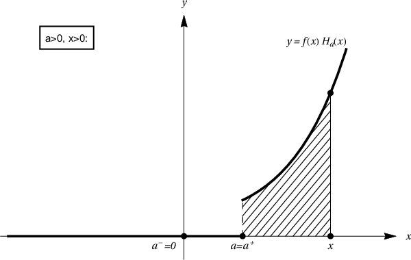
The motivation for definition (6) comes from the standard example $\mathcal{F}=C^{\infty}(\mathbbm{R})$ where it reproduces the usual Riemann integral ${\textstyle\int}={\textstyle\int}_{\!0}^{x}$. This is illustrated in Figure 1, where we have visualized ${\textstyle\int}fH_{a}$ with $f(x)=\cosh{x}$ in the four different cases corresponding to the signs of $x$ and $a$. While both forms of (6) are obvious from the figure, their identity is a general fact of ordinary shifted integro-differential algebras $\mathcal{F}$ as one can see by a straightforward calculation using the generic relations (9) mentioned below.

In a similar way we can also define the shifts $S_{a}\colon\mathcal{P}\mathcal{F}\to\mathcal{P}\mathcal{F}$. Since in the standard examples, $f(x)\mapsto f(x+a)$ shifts the graph of $f$ by $a$ units to the left, we are led to $S_{a}(H_{b}):=H_{b-a}$. This fixes $S_{a}\colon\mathcal{P}\mathcal{F}\to\mathcal{P}\mathcal{F}$ in view of (5) by requiring it to be an algebra homomorphism extending the given shifts $S_{a}\colon\mathcal{F}\to\mathcal{F}$. Obviously, the group law $S_{a}\circ S_{b}=S_{a+b}$ is satisfied.

Finally, we define $\text{{e}}\colon\mathcal{P}\mathcal{F}\to K$ as the unique character extending $\text{{e}}\colon\mathcal{F}\to K$ by the equivalent stipulations $\text{{e}}(H_{a})=\bar{H}(a)$ or $\text{{e}}(\bar{H}_{a})=H(a)$. Using again $\text{{e}}_{c}:=\text{{e}}\circ S_{c}\colon\mathcal{P}\mathcal{F}\to K$ as shorthand notation, we have also $\text{{e}}_{c}(H_{a})=\bar{H}(a-c)$ and $\text{{e}}_{c}(\bar{H}_{a})=H(a-c)$. At this point it should be noted that we could also use the right continuous convention for the Heaviside operator $H(a)$ but not the symmetric one: Indeed, the relation $H_{a}H_{b}=H_{a\sqcup b}$ implies $\bar{H}(a)\,\bar{H}(b)=\bar{H}(a\sqcup b)$, which is satisfied by all three conventions if $(a,b)\neq(0,0)$; but the remaining case $\bar{H}(0)^{2}=\bar{H}(0)$ entails $\bar{H}(0)\in\{0,1\}$ and thus rules out the symmetric convention.⁷⁷ 7 We can only see one apparent advantage of the symmetric convention, in trying to build up a derivation with a Leibniz rule for Heavisides—but even this is ultimately doomed to fail: see Remark 13. It is easy to check that e is indeed an evaluation on $(\mathcal{P}\mathcal{F},{\textstyle\int})$.

As for any monoid algebra (Lang, 2002, p. 106), the map $\mathcal{F}\to\mathcal{F}[K_{\sqcup}],\>f\mapsto f\cdot 1_{\mathcal{P}\mathcal{F}}$ is an embedding, hence $\mathcal{F}$ is a $K$-subalgebra of $\mathcal{P}\mathcal{F}=\mathcal{F}[K_{\sqcup}]$. Since the Rota-Baxter operator on $\mathcal{P}\mathcal{F}$ has been defined as an extension, $(\mathcal{P}\mathcal{F},{\textstyle\int})$ is indeed a Rota-Baxter extension of $(\mathcal{F},{\textstyle\int})$.

We have already seen that the $S_{a}\colon\mathcal{P}\mathcal{F}\to\mathcal{P}\mathcal{F}$ defined above yield a shift map on $\mathcal{P}\mathcal{F}$, and that the character $\text{{e}}\colon\mathcal{P}\mathcal{F}\to K$ defined above is an evaluation on $(\mathcal{P}\mathcal{F},{\textstyle\int})$. Hence it remains to prove the compatibility relation $[S_{c},{\textstyle\int}]=\text{{e}}_{c}{\textstyle\int}$ for the induced evaluations $\text{{e}}_{c}=\text{{e}}\circ S_{c}$. By (5), we need only verify the relation on elements of the form $fH_{a}\in\mathcal{P}\mathcal{F}$; we know it is satisfied for $f\in\mathcal{F}$ due to the shift relation on $\mathcal{F}$. The verification may be done by a four-fold case distinction based on the positivity of $a$ and $a-c$. For an alternative direct proof one employs the generic identities (valid for Rota-Baxter algebras over ordered fields)

together with the simple consequence ${\textstyle\int}_{\!0}^{a-c}S_{c}f={\textstyle\int}_{\!c}^{a}f$ of the shift relation on $\mathcal{F}$. Doing so yields ${\textstyle\int}_{\!0}^{c}f+H(a)\,{\textstyle\int}_{\!a}^{0}f+H(a-c)\,{\textstyle\int}_{\!c}^{a}f$ for both sides of $[S_{c},{\textstyle\int}]fH_{a}=\text{{e}}_{c}{\textstyle\int}fH_{a}$. $\Box$ 

We have now an algebraic description of integration on rings of piecewise functions, constructed from Heavisides. If all functions are piecewise smooth (cf. Example 7), we can add a derivation $\partial$ to obtain a differential Rota-Baxter algebra that is, however, not an integro-differential algebra (Proposition 6). Normally, only in the latter case do we speak of an induced evaluation $\text{{e}}:=1_{\mathcal{F}}-{\textstyle\int}\partial$, but since the analogous concept is also useful in differential Rota-Baxter algebras we introduce this operation now in the general context.

Assume now that $(\mathcal{F},\partial,{\textstyle\int})$ is a differential Rota-Baxter algebra such that $(\mathcal{F},{\textstyle\int})$ satisfies the conditions of Proposition 4. Then we define a derivation on the piecewise extension $\mathcal{P}\mathcal{F}$ by extending the derivation on $\mathcal{F}$ by zero. In other words, we set $\partial H_{a}=0$ for all $a\in K$; then $\partial\colon\mathcal{P}\mathcal{F}\to\mathcal{P}\mathcal{F}$ is uniquely determined by the Leibniz rule. Note that the ring of constants is enlarged to $\operatorname{Ker}(\partial)=K[H_{a}\mid a\in K]$. This reflects the viewpoint of analysis that the derivative of the Heaviside function $H(x-a)\in L^{2}(\mathbbm{R})$ vanishes. Of course, this is in stark contrast to the more ambitious treatment via distributions taken up in the next section (where the simple derivation from above is no longer in use).

One checks immediately that the pseudo-evaluation of $\mathcal{P}\mathcal{F}$ is given by (10), using the handy relation $\text{{e}}_{a}=\text{{e}}_{a^{+}}-\text{{e}}_{0}+\text{{e}}_{a^{-}}$. As for every integro-differential algebra, we have $(K[x],{\textstyle\int})\subseteq(\mathcal{F},{\textstyle\int})$. Since $K\supseteq\mathbbm{Q}$ is an ordered field, we have $0<1<2$ so that

which shows that $\hat{\text{{e}}}$ fails to be multiplicative. $\Box$ 

As a special case of (10), note that $\hat{\text{{e}}}(H_{a})=H_{a}$. This is in agreement with the fact that the constants are given by $\operatorname{Ker}(\partial)=K[H_{a}\mid a\in K]$; we see $H_{a}$ as a differential constant that pseudo-evaluates to itself. Of course one must be careful not to confuse the pseudo-evaluation with the distinguished evaluation $\text{{e}}(H_{a})=\bar{H}(a)$, which has image $K$ rather than $K[H_{a}\mid a\in K]$. This shows also that Proposition 4 cannot be strengthened to yield an ordinary Rota-Baxter algebra $(\mathcal{P}\mathcal{F},{\textstyle\int})$. Indeed, even when ${\textstyle\int}$ is injective as in Proposition 6, the complement of its image is larger than the ground field $K$.

Piecewise defined functions are a major motivation for introducing distributions, via generalized derivatives. In particular, we will no longer view $\partial H_{a}$ as identically zero but as a “Dirac delta” $\delta_{a}$, sometimes written $\delta_{a}(x)=\delta(x-a)$. Again we shall pursue a purely algebraic route to introduce these quantities along with an integro-differential structure.

The basic property of the Dirac distribution $\delta_{a}$ concentrated at a source point $a$ is that its only nonzero “value” is assumed for $x=a$, in the sense that $f\delta_{a}$ vanishes identically when $f(a)=0$. In other words, $f\delta_{a}$ only depends on $f(a)$ and not on all of $f$, and one has the sifting property

for ‘‘extracting’’ the source value. This will be the basis of our algebraic construction.¹⁰¹⁰ 10 Using $\mathcal{P}\mathcal{F}\,\{\delta_{a}\mid a\in K\}_{1}$ instead of $\mathcal{F}\{H_{a}\mid a\in K\}_{1}$ may seem more natural and incremental, but it runs into problems with the Leibniz rule: see Remark 13.

Recall that $\mathcal{F}\{X\}_{1}$ denotes the module of affine differential polynomials in $X$. We have also employed the abbreviation $\delta_{a}:=H_{a}^{\prime}$, which we shall continue to use throughout this paper (of course derivatives $\eth\varphi$ of $\varphi\in\mathcal{D}\mathcal{F}$ are also denoted by $\varphi^{\prime}$). The order on $K$ induces an elimination ranking $\prec$ on $\mathcal{F}\{H_{a}\mid a\in K\}$ and thus a Noetherian term order on the $\mathcal{F}$-module $\mathcal{F}\{H_{a}\mid a\in K\}_{1}$. We have $H_{a}^{(m)}\prec H_{b}^{(n)}$ iff $a<b$ or otherwise $a=b$ and $m<n$. In the sequel we shall always employ this term order on the free differential module underlying $\mathcal{D}\mathcal{F}$. It is easy to get a kind of Gröbner basis for $Z$ with respect to this term order. Moreover, the direct decomposition

References

- Bergman (1978) G.M. Bergman. The diamond lemma for ring theory. Advances in Mathematics, 29(2):179–218, August 1978.
- Buchberger (2006) B. Buchberger. Bruno Buchberger’s PhD thesis 1965: An algorithm for finding the basis elements of the residue class ring of a zero dimensional polynomial ideal. J. Symbolic Comput., 41(3-4):475–511, 2006. Translated from the 1965 German original by Michael P. Abramson.
- Buchberger, Rosenkranz (2012) B. Buchberger and M. Rosenkranz. Transforming problems from analysis to algebra: a case study in linear boundary problems. J. Symbolic Comput., 47(6):589–609, 2012.
- Duistermaat, Kolk (2010) J.J. Duistermaat and J.A.C. Kolk. Distributions. Cornerstones. Birkhäuser Boston Inc., Boston, MA, 2010. Theory and applications, Translated from the Dutch by J. P. van Braam Houckgeest.
- Gao, Guo, Rosenkranz (2015) X. Gao, L. Guo, and M. Rosenkranz. On rings of differential rota-baxter operators. Preprint on arXiv:1512.01247, December 2015.
- Graham, Knuth, Patashnik (1994) R.L. Graham, D.E. Knuth, and O. Patashnik. Concrete mathematics. Addison-Wesley Publishing Company, Reading, MA, second edition, 1994. A foundation for computer science.
- Guo (2012) L. Guo. An Introduction to Rota-Baxter Algebras. International Press, 2012.
- Guo, Keigher (2008) L. Guo and W. Keigher. On differential Rota-Baxter algebras. J. Pure Appl. Algebra, 212(3):522–540, 2008.
- Guo, Regensburger, Rosenkranz (2012) L. Guo, G. Regensburger, and M. Rosenkranz. On integro-differential algebras. Journal of Pure and Applied Algebra, 218(3):456–473, March 2014.
- Kato, Struppa (1999) G. Kato and D.C. Struppa. Fundamentals of Algebraic Microlocal Analysis. Pure and Applied Mathematics. Marcel Dekker Inc., 1999.
- Kolchin (1973) E.R. Kolchin. Differential algebra and algebraic groups, volume 54 of Pure and Applied Mathematics. Academic Press, New York-London, 1973.
- Lang (2002) S. Lang. Algebra, volume 211 of Graduate Texts in Mathematics. Springer-Verlag, third edition, 2002.
- MacLane, Birkhoff (1968) S. MacLane and G. Birkhoff. Algebra. MacMillan, New York, 1968.
- Put, Singer (2003) M. van der Put and M.F. Singer. Galois theory of linear differential equations, volume 328 of Grundlehren der Mathematischen Wissenschaften. Springer, Berlin, 2003.
- Regensburger, Rosenkranz (2009) G. Regensburger and M. Rosenkranz. An algebraic foundation for factoring linear boundary problems. Ann. Mat. Pura Appl. (4), 188(1):123–151, 2009.
- Regensburger, Rosenkranz (2009) G. Regensburger and M. Rosenkranz. Symbolic integral operators and boundary problems. Lecture Notes, 2009.
- Ritt (1966) J.F. Ritt. Differential algebra. Dover, New York, 1966.
- Robertz (2014) D. Robertz. Formal Algorithmic Elimination for PDEs, volume 2121 of Lecture Notes in Mathematics. Springer, 2014.
- Rosenkranz, Gao, Guo (2015) M. Rosenkranz, X. Gao, and L. Guo. An algebraic study of multivariable integration and linear substitution. Technical Report 1503.01694, arXiv, 2015.
- Rosenkranz, Korporal (2013) M. Rosenkranz and A. Korporal. A noncommutative algebraic operational calculus for boundary problems. Math. Comput. Sci., 7:201–227, 2013.
- Rosenkranz Regensburger (2008) M. Rosenkranz and G. Regensburger. Solving and factoring boundary problems for linear ordinary differential equations in differential algebras. Journal of Symbolic Computation, 43(8):515–544, 2008.
- Rosenkranz, Serwa (2015) M. Rosenkranz and N. Serwa. Green’s functions for stieltes boundary problems. In ISSAC, 2015. to appear.
- Schwartz (1954) L. Schwartz. Sur l’impossibilité de la multiplication des distributions. Comptes Rendus de L’Académie des Sciences, 239:847–848, 1954.
- Seiler (1997) W. Seiler. Computer algebra and differential equations: An overview. mathPAD, 7:34–49, 1997.
- Stakgold, Holst (2011) I. Stakgold and M. Holst. Green’s functions and boundary value problems. Pure and Applied Mathematics (Hoboken). John Wiley & Sons, Inc., Hoboken, NJ, third edition, 2011.