跳到论文正文
W Papers独立论文阅读器 arXiv:1707.06512 论文正文 计算阅读时间 · 0%
引用这篇论文根据当前论文元数据生成,正式投稿前建议核对。


License: arXiv.org perpetual non-exclusive license
arXiv:1707.06512v2 [cond-mat.other] 07 Aug 2017

Theory of ground states for classical Heisenberg spin systems III

Heinz-Jürgen Schmidt1 Note: Correspondence should be addressed to hschmidt@uos.de Address: 1Universität Osnabrück, Fachbereich Physik, Barbarastr. 7, D - 49069 Osnabrück, Germany
Abstract

We extend the theory of ground states of classical Heisenberg spin systems published previously by a closer investigation of the convex Gram set of NN spins. This is relevant for the present purpose since the set of ground states of a given spin system corresponds to a face of the Gram set. The investigation of the Gram set is facilitated by the determination of its symmetry group. The case of the general spin triangle is completely solved and illustrated by a couple of examples.

I Introduction

This is the third of a series of papers devoted to the theory of ground states of finite classical Heisenberg spin systems. The general motivation of such a theory can be found in [1] and need not be repeated here. Extended examples are contained in [2]. In section II.1 we will recapitulate the central definitions and results of the “Lagrange variety approach" presented in [1]. The system of NN spins will be described by a symmetric N×NN\times N-matrix 𝕁⁡(𝝀){\mathbbm{J}}({\boldsymbol{\lambda}}) depending on an N−1N-1-dimensional vector 𝝀∈Λ{\boldsymbol{\lambda}}\in\Lambda. The MM-dimensional ground states 𝐬{\mathbf{s}} lives in the eigenspace of 𝕁⁡(𝝀){\mathbbm{J}}({\boldsymbol{\lambda}}) corresponding to the minimal eigenvalue jm​i​n​(𝝀^)j_{min}(\hat{\boldsymbol{\lambda}}) and a unique point 𝝀^∈Λ\hat{\boldsymbol{\lambda}}\in\Lambda where jm​i​n​(𝝀^)j_{min}(\hat{\boldsymbol{\lambda}}) assumes its maximum. They can be further characterized by the “degree of additional degeneracy" dd and “co-degree" pp such that p+d=12​M​(M+1)p+d=\frac{1}{2}M(M+1).
Then, in section II.2 we present the “Gram set approach" to the ground state problem that yields further insights. Each spin configuration 𝐬{\mathbf{s}} can also be described by its Gram matrix G⁡(𝐬)G({\mathbf{s}}) such that different spin configurations that are equivalent w. r. t. rotations/reflections yield the same Gram matrix and vice versa. The convex set of all such N×NN\times N-Gram matrices is denoted by 𝒢N{\mathcal{G}}_{N}. The energy function can be written as an affine functional 𝒢N⟶ℝ{\mathcal{G}}_{N}\longrightarrow{\mathbbm{R}} defined by G↦Tr ​G​𝕁G\mapsto\mbox{Tr }G\,{\mathbbm{J}}. Hence the set of ground states of 𝕁{\mathbbm{J}} corresponds to the face FF of 𝒢N{\mathcal{G}}_{N} where G↦Tr ​G​𝕁G\mapsto\mbox{Tr }G\,{\mathbbm{J}} assumes its minimum. The afore-mentioned degree dd equals the dimension of FF. This leads to a more global angle of view: Instead of asking, which are the ground states of a given 𝕁{\mathbbm{J}}, we rather analyze the faces FF of 𝒢N{\mathcal{G}}_{N} and look for the set of matrices 𝕁{\mathbbm{J}} such that G↦Tr ​G​𝕁G\mapsto\mbox{Tr }G\,{\mathbbm{J}} assumes its minimum at FF.

Further topics of this section are the definition of symmetries of the Gram set that are generated by permutations of spins and partial reflections and the geometry of “Ising matrices", i. e., those Gram matrices that correspond to one-dimensional spin configurations.

Next we apply the combined Lagrange variety and Gram set approach to the ground state problem of the general classical spin triangle, i. e., for N=3N=3. Here it is possible to visualize the Gram set and its faces in a 33-dimensional plot. The ground state problem can be explicitly solved for N=3N=3. That means that given the three coupling constants one can determine the corresponding face FF and calculate all ground states 𝐬{\mathbf{s}} such that G⁡(𝐬)∈FG({\mathbf{s}})\in F. In the Appendix A we calculate all completely elliptic subspaces of ℝ3{\mathbbm{R}}^{3}. This set is in 1:11:1 correspondence to the set of closed faces of 𝒢3{\mathcal{G}}_{3}. A second Appendix B is devoted to the proof that the above-mentioned symmetries of the Gram set are the only ones. We close with a summary and outlook.

II General definitions and results

II.1 Lagrange variety approach

The classical phase space 𝒫M{\mathcal{P}}_{M} for the systems of NN spins under consideration consists of all configurations of MM-dimensional spin vectors

𝐬μ,μ=1,…,N,\mathbf{s}_{\mu},\;\mu=1,\ldots,N\;, (1)

subject to the constraints

𝐬μ⋅𝐬μ=1,μ=1,…,N,\mathbf{s}_{\mu}\cdot\mathbf{s}_{\mu}=1,\;\mu=1,\ldots,N\;, (2)

where ⋅\cdot denotes the usual inner product of ℝM{\mathbb{R}}^{M}. Hence 𝒫M{\mathcal{P}}_{M} can be considered as the NN-fold product of unit spheres, 𝒫M=𝒮(M−1)×…×𝒮(M−1){\mathcal{P}}_{M}={\mathcal{S}}^{(M-1)}\times\ldots\times{\mathcal{S}}^{(M-1)}. We write the elements 𝐬{\mathbf{s}} of 𝒫M{\mathcal{P}}_{M} as N×MN\times M-matrices with entries 𝐬μ,i,μ=1,…,N,i=1,…,M{\mathbf{s}}_{\mu,i},\;\mu=1,\ldots,N,\;i=1,\ldots,M. Hence 𝐬{\mathbf{s}} has NN rows 𝐬μ,μ=1,…,N{\mathbf{s}}_{\mu},\,\mu=1,\ldots,N and MM columns 𝐬i,i=1,…,M{\mathbf{s}}_{i},\,i=1,\ldots,M. The “dimension of 𝐬{\mathbf{s}}" is defined as its matrix rank,  dim ​𝐬≡ rank ​𝐬\mbox{ dim }{{\mathbf{s}}}\equiv\mbox{ rank }{{\mathbf{s}}}. A subspace S⊂ℝNS\subset{\mathbbm{R}}^{N} is called “MM-elliptic" iff there exists an N×MN\times M-matrix 𝐬{\mathbf{s}} such that its columns 𝐬i∈S{\mathbf{s}}_{i}\in S for i=1,…,Mi=1,\ldots,M and its rows 𝐬μ,μ=1,…,N{\mathbf{s}}_{\mu},\,\mu=1,\ldots,N satisfy (2). In other words, there exists an MM-dimensional spin configuration living on SS. SS is called “elliptic" if it is MM-elliptic for some M>0M>0 and “completely elliptic" iff there exists an N×MN\times M-matrix 𝐬{\mathbf{s}} such that its columns 𝐬i∈S{\mathbf{s}}_{i}\in S for i=1,…,Mi=1,\ldots,M and its rows 𝐬μ,μ=1,…,N{\mathbf{s}}_{\mu},\,\mu=1,\ldots,N satisfy (2), and moreover, rank ​𝐬= dim ​S=M\mbox{rank }{\mathbf{s}}=\mbox{ dim }S=M. If SS is elliptic and r=rank ​𝐬<Mr=\mbox{rank }{\mathbf{s}}<M then we may choose a suitable rotation R∈O⁡(M)R\in O(M) such that 𝐬′=𝐬​R{\mathbf{s}}^{\prime}={\mathbf{s}}\,R has only rr non-zero columns. After deleting the zero columns we obtain r=rank ​𝐬′=Mr=\mbox{rank }{\mathbf{s}}^{\prime}=M. Further restricting SS to the subspace S′S^{\prime} spanned by the columns of 𝐬′{\mathbf{s}}^{\prime} then yields a completely elliptic subspace.

The Heisenberg Hamiltonian HH is a smooth function defined on 𝒫M{\mathcal{P}}_{M} of the form

H⁡(𝐬)=∑μ,ν=1NJμ​ν​𝐬μ⋅𝐬ν,H(\mathbf{s})=\sum_{\mu,\nu=1}^{N}J_{\mu\nu}\,\mathbf{s}_{\mu}\cdot\mathbf{s}_{\nu}\;, (3)

where the coupling coefficients Jμ​νJ_{\mu\nu} are the entries of a real, symmetric N×NN\times N matrix 𝕁\mathbb{J} with vanishing diagonal. We will denote by 𝒮​ℳ​(N){\mathcal{S}}{\mathcal{M}}(N) the linear space of real, symmetric N×NN\times N matrices. A “ground state" of the spin system is defined as any configuration 𝐬\mathbf{s} where H⁡(𝐬)H({\mathbf{s}}) assumes a global minimum Em​i​nE_{min}. In general there exist a lot of ground states. For example, a global rotation/reflection of a ground state is again a ground state due to the invariance of the Hamiltonian (3) under rotations/reflections. Recall that the group of all invertible M×MM\times M-matrices RR satisfying R−1=R⊤R^{-1}=R^{\top} is denoted by O⁡(M)O(M). In general we will call two spin configurations 𝐬{\mathbf{s}} and 𝐬′{\mathbf{s}}^{\prime} “O⁡(M)O(M)-equivalent" iff there exists an R∈O⁡(M)R\in O(M) such that 𝐬μ′=R​𝐬μ{\mathbf{s}}^{\prime}_{\mu}=R\,{\mathbf{s}}_{\mu} for all μ=1,…,N\mu=1,\ldots,N. Further degeneracies of the ground states apart from the “trivial" rotational/reflectional degeneracy will be called “additional degeneracies".

Any ground state 𝐬{\mathbf{s}} satisfies the “stationary state equation" (SSE)

𝕁⁡(𝜿)​𝐬=0.{\mathbb{J}}({\boldsymbol{\kappa}})\,{\mathbf{s}}=0. (4)

Here 𝕁⁡(𝜿)∈𝒮​ℳ​(N)​𝒮​ℳ​(N){\mathbb{J}}({\boldsymbol{\kappa}})\in{\mathcal{S}}{\mathcal{M}}(N){\mathcal{S}}{\mathcal{M}}(N) is the “dressed 𝕁\mathbb{J}-matrix" with entries

(𝕁⁡(𝜿))μ​ν=Jμ​ν+κμ​δμ​ν,\left({\mathbb{J}}(\boldsymbol{\kappa})\right)_{\mu\nu}=J_{\mu\nu}+\kappa_{\mu}\,\delta_{\mu\nu}\;, (5)

where 𝜿∈ℝN{\boldsymbol{\kappa}}\in{\mathbbm{R}}^{N} and its components κμ\kappa_{\mu} are the (negative) NN Lagrange parameters due to the constraints (2). The “undressed" matrix 𝕁{\mathbb{J}} without 𝜿{\boldsymbol{\kappa}} will always denote a symmetric N×NN\times N-matrix with zero diagonal. As in [1] we may split the Lagrange parameters κμ\kappa_{\mu} into the mean value κ¯\bar{\kappa} and the deviations λμ\lambda_{\mu} from the mean value according to

κ¯\displaystyle\bar{\kappa} ≡\displaystyle\equiv 1N​∑μ=1Nκμ,\displaystyle\frac{1}{N}\sum_{\mu=1}^{N}\,\kappa_{\mu}, (6)
λμ\displaystyle\lambda_{\mu} ≡\displaystyle\equiv κμ−κ¯.\displaystyle\kappa_{\mu}-\bar{\kappa}\;. (7)

We denote by Λ\Lambda the (N−1)(N-1)-dimensional subspace of vectors 𝝀∈ℝN{\boldsymbol{\lambda}}\in{\mathbb{R}}^{N} satisfying ∑μ=1Nλμ=0\sum_{\mu=1}^{N}\lambda_{\mu}=0. Then (4) can be written in the form of an eigenvalue equation:

𝕁(𝝀)𝐬i=−κ¯𝐬i,i=1,…,M.{\mathbb{J}}({\boldsymbol{\lambda}})\,{\mathbf{s}}_{i}=-\bar{\kappa}\,{\mathbf{s}}_{i},\;i=1,\ldots,M. (8)

The energy (3) does not change if the undressed 𝕁{\mathbb{J}}-matrix is replaced by 𝕁⁡(𝝀){\mathbb{J}}({\boldsymbol{\lambda}}). We introduce some more notation. Let jα​(𝝀)j_{\alpha}({\boldsymbol{\lambda}}) denote the α−\alpha-th eigenvalue of 𝕁⁡(𝝀){\mathbb{J}}({\boldsymbol{\lambda}}) and jm​i​n​(𝝀)j_{min}({\boldsymbol{\lambda}}) its lowest eigenvalue for 𝝀∈Λ{\boldsymbol{\lambda}}\in\Lambda. Then the following holds:

Theorem 1

Under the preceding definitions there exists a unique point 𝛌^∈Λ\hat{\boldsymbol{\lambda}}\in\Lambda such that jm​i​n​(𝛌)j_{min}({\boldsymbol{\lambda}}) assumes its maximum ȷ^\hat{\jmath} at 𝛌^\hat{\boldsymbol{\lambda}} and the corresponding eigenspace SS of 𝕁⁡(𝛌^){\mathbb{J}}(\hat{\boldsymbol{\lambda}}) is elliptic. Moreover, all ground states of (3) live on SS.

This follows from the theorems 1,2,3 of [1].

Now consider an M′′M^{\prime\prime}-elliptic subspace S′S^{\prime}, for example the eigenspace of (𝕁⁡(𝝀^),ȷ^)({\mathbb{J}}(\hat{\boldsymbol{\lambda}}),\hat{\jmath}) according to Theorem 2. Let W′W^{\prime} denote an N×M′N\times M^{\prime}-matrix such that the M′M^{\prime} columns of W′W^{\prime} form a basis of S′S^{\prime}, hence M′= dim ​S′M^{\prime}=\mbox{ dim }S^{\prime}. W′W^{\prime} can be viewed as an injective linear map W′:ℝM′⟶ℝNW^{\prime}:{\mathbbm{R}}^{M^{\prime}}\longrightarrow{\mathbbm{R}}^{N} and, similarly, W′⁣⊤W^{\prime\top} as a surjective linear map W′⁣⊤:ℝN⟶ℝM′W^{\prime\top}:{\mathbbm{R}}^{N}\longrightarrow{\mathbbm{R}}^{M^{\prime}}.

According to the definition of “M′′M^{\prime\prime}-elliptic" there exists a spin configuration 𝐬{\mathbf{s}} such that the columns 𝐬i∈S′{\mathbf{s}}_{i}\in S^{\prime} for i=1,…,M′′i=1,\ldots,M^{\prime\prime}. These columns are unique linear combinations of the basis vectors Wj′,j=1,…​M′W^{\prime}_{j},\;j=1,\ldots M^{\prime}, i. e. ,

𝐬μ​i=∑j=1M′W′μ​jΓj​i,i=1,…,M′′,μ=1,…,N.{\mathbf{s}}_{\mu i}=\sum_{j=1}^{M^{\prime}}W^{\prime}_{\mu j}\,\Gamma_{j\,i},\quad i=1,\ldots,M^{\prime\prime},\;\mu=1,\ldots,N. (9)

In matrix notation (9) is written as 𝐬=W′​𝚪{\mathbf{s}}=W^{\prime}\;{\boldsymbol{\Gamma}}, where 𝚪{\boldsymbol{\Gamma}} is the M′×M′′M^{\prime}\times M^{\prime\prime}-matrix with entries Γj​i\Gamma_{j\,i}. The condition (2) that the rows 𝐬μ{\mathbf{s}}_{\mu} of 𝐬{\mathbf{s}} are unit vectors assumes the form

1=(𝐬​𝐬⊤)μ​μ=(W′​𝚪​𝚪⊤​W′⁣⊤)μ​μ=(W′​𝚫′​W′⁣⊤)μ​μ,1=\left({\mathbf{s}}\,{\mathbf{s}}^{\top}\right)_{\mu\mu}=\left(W^{\prime}\,{\boldsymbol{\Gamma}}\,{\boldsymbol{\Gamma}}^{\top}\,W^{\prime\top}\right)_{\mu\mu}=\left(W^{\prime}\,{\boldsymbol{\Delta}}^{\prime}\,W^{\prime\top}\right)_{\mu\mu}, (10)

where 𝚫′≡𝚪​𝚪⊤{\boldsymbol{\Delta}}^{\prime}\equiv{\boldsymbol{\Gamma}}\,{\boldsymbol{\Gamma}}^{\top} is a positively semi-definite M′×M′M^{\prime}\times M^{\prime}-matrix. Let 𝒮′{\mathcal{S}}^{\prime} be the set of solutions 𝚫′≥0{\boldsymbol{\Delta}}^{\prime}\geq 0 of (10). According to the assumption of ellipticity this solution set is not empty. Generally, 𝒮′{\mathcal{S}}^{\prime} is the intersection of the affine space of solutions of (10) with the closed convex cone 𝒮​ℳ+​(M′){\mathcal{S}}{\mathcal{M}}_{+}(M^{\prime}) of positively semi-definite M′×M′M^{\prime}\times M^{\prime}-matrices, and hence a closed convex set. Let F=𝖿𝖺𝖼𝖾⁡(𝒮′)F={\sf face}\left({\mathcal{S}}^{\prime}\right), the face of 𝒮​ℳ+​(M′){\mathcal{S}}{\mathcal{M}}_{+}(M^{\prime}) generated by the subset 𝒮′{\mathcal{S}}^{\prime}. According to Theorem 2, see section II.2, FF is of the form 𝖿𝖺𝖼⁡(U){\sf fac}(U), where UU is a linear subspace of ℝM′{\mathbbm{R}}^{M^{\prime}}. and 𝖿𝖺𝖼⁡(U){\sf fac}(U) is the face of all positively semi-definite M′×M′M^{\prime}\times M^{\prime}-matrices that live on UU. Let M= dim ​UM=\mbox{ dim }U. Further define S≡W′[U]≡{W′u|u∈U}S\equiv W^{\prime}[U]\equiv\{W^{\prime}\,u\left|u\in U\right.\}. Here W′W^{\prime} is considered as an injective linear map, see above, hence dim ​S=dim ​U=M\mbox{dim }S=\mbox{dim }U=M. Without loss of generality we may assume that the first MM columns of W′W^{\prime} form a basis of SS. Let WW denote the corresponding N×MN\times M-submatrix of W′W^{\prime}, and 𝚫{\boldsymbol{\Delta}} the correspondingly truncated M×MM\times M-submatrix of 𝚫′{\boldsymbol{\Delta}}^{\prime}. Then (10) assumes the form

1=(W​𝚫​W⊤)μ​μ.1=\left(W\,{\boldsymbol{\Delta}}\,W^{\top}\right)_{\mu\mu}. (11)

Let 𝒮{\mathcal{S}} denote the set of solutions 𝚫≥0{\boldsymbol{\Delta}}\geq 0 of (11). It is essentially the same set as 𝒮′{\mathcal{S}}^{\prime} but now the solutions are considered as M×MM\times M-matrices. Usually 𝒮{\mathcal{S}} is represented by the convex range 𝒮p​a​r{\mathcal{S}}_{par} of suitable parameters. If all solutions 𝚫∈𝒮{\boldsymbol{\Delta}}\in{\mathcal{S}} would have  rank ​𝚫<M\mbox{ rank }{\boldsymbol{\Delta}}<M then they would generate a face of 𝒮​ℳ+​(M){\mathcal{S}}{\mathcal{M}}_{+}(M) that is smaller than F=𝖿𝖺𝖼⁡(U)F={\sf fac}(U) which contradicts the definition of FF. Hence there exists some 𝚫0∈𝒮{\boldsymbol{\Delta}}_{0}\in{\mathcal{S}} with  rank ​𝚫0=M\mbox{ rank }{\boldsymbol{\Delta}}_{0}=M and consequently 𝚫0>0{\boldsymbol{\Delta}}_{0}>0. It follows that 𝐬≡W​𝚫0{\mathbf{s}}\equiv W\,\sqrt{{\boldsymbol{\Delta}}_{0}} is a spin configuration, i. e., satisfying (2), with  rank ​𝐬= dim ​𝐬=M\mbox{ rank }{\mathbf{s}}=\mbox{ dim }{\mathbf{s}}=M. (For the proof of the latter statement, let x≠0x\neq 0 be a vector satisfying 𝐬​x=0{\mathbf{s}}\,x=0, then y≡𝚫0​x≠0y\equiv\sqrt{{\boldsymbol{\Delta}}_{0}}\,x\neq 0 satisfies W​y=0W\,y=0, i. e. , the columns of WW are linearly dependent. This is a contradiction to the assumption that the columns of WW form a basis of SS.)

In this way we have shown that every elliptic subspace S′⊂ℝNS^{\prime}\subset{\mathbbm{R}}^{N} contains a completely elliptic subspace S⊂S′S\subset S^{\prime}. In section III we will give an example of SS being a proper subspace of S′S^{\prime} in the context of the spin triangle. In accordance with [1] we will call (11) together with the condition 𝚫≥0{\boldsymbol{\Delta}}\geq 0 the “additional degeneracy equation" (ADE). It has been shown in [1] that its solution set 𝒮=𝒮A​D​E{\mathcal{S}}={\mathcal{S}}_{ADE} is of the form 𝒮=(Δ0+P⟂)∩𝒮​ℳ+​(M){\mathcal{S}}=\left(\Delta_{0}+P^{\perp}\right)\cap{\mathcal{S}}{\mathcal{M}}_{+}(M). Here PP is the subspace of 𝒮​ℳ​(M){\mathcal{S}}{\mathcal{M}}(M) spanned by the the rank 11 matrices Pμ,μ=1,…,N,P_{\mu},\mu=1,\ldots,N,. They are defined as the projectors onto the 11-dimensional subspaces spanned by the μ\mu-th row WμW_{\mu} of WW multiplied by ‖Wμ‖2\|W_{\mu}\|^{2}. The orthogonal complement P⟂P^{\perp} of PP is defined w. r. t. the inner product ⟨A|B⟩≡Tr​(A​B)\langle A|B\rangle\equiv\mbox{Tr}\left(A\,B\right) of 𝒮​ℳ​(M){\mathcal{S}}{\mathcal{M}}(M). It follows [1] that 𝒮{\mathcal{S}} is a dd-dimensional closed convex set where the “degree dd" of SS is defined by d≡M⁡(M+1)/2−pd\equiv M(M+1)/2\,-\,p, and the “co-degree pp" of SS by p≡dim ​Pp\equiv\mbox{dim }P.

We stress that the solution set 𝒮{\mathcal{S}} depends on the choice of the matrix WW and the latter is, in general, not unique. The condition that the MM columns of WW form a basis of SS allows that WW can be replaced by W​AW\,A, where AA is some invertible M×MM\times M-matrix. This induces the transformation 𝚫↦A​𝚫​A−1{\boldsymbol{\Delta}}\mapsto A\,{\boldsymbol{\Delta}}\,A^{-1} of 𝒮{\mathcal{S}} which is an affine bijection 𝒮⟶𝒮~{\mathcal{S}}\longrightarrow\widetilde{\mathcal{S}}.

II.2 Gram set approach

II.2.1 Generalities

We will recapitulate and generalize some notions already introduced in [3] and [1]. For each spin configuration 𝐬{\mathbf{s}} we define the “Gram matrix" G=G⁡(𝐬)≡𝐬​𝐬⊤G=G({\mathbf{s}})\equiv{\mathbf{s}}\,{\mathbf{s}}^{\top} with entries Gμ​ν=𝐬μ⋅𝐬νG_{\mu\nu}={\mathbf{s}}_{\mu}\cdot{\mathbf{s}}_{\nu}. Hence GG will be a symmetric N×NN\times N-matrix that is positively semi-definite, G≥0G\geq 0, and satisfies Gμ​μ=1G_{\mu\mu}=1 for all μ=1,…,N\mu=1,\ldots,N. Moreover, rank ​(G)=rank ​(𝐬)≤N\mbox{rank }(G)=\mbox{rank }({\mathbf{s}})\leq N.

Conversely, if GG is a positively semi-definite N×NN\times N-matrix with rank ​G=M≤N\mbox{rank }G=M\leq N, satisfying Gμ​μ=1G_{\mu\mu}=1 for all μ=1,…,N\mu=1,\ldots,N, then 𝐬≡G{\mathbf{s}}\equiv\sqrt{G} defines a spin configuration such that G=G⁡(𝐬)G=G({\mathbf{s}}). The correspondence between spin configurations 𝐬{\mathbf{s}} and Gram matrices is many-to-one: Let R∈O⁡(M)R\in O(M) be a rotation/reflection, then the two configurations 𝐬μ{\mathbf{s}}_{\mu} and R​𝐬μ,μ=1,…,N,R\,{\mathbf{s}}_{\mu},\;\mu=1,\ldots,N, will obviously yield the same Gram matrix. Conversely, if G⁡(𝐬)=G⁡(𝐬′)G({\mathbf{s}})=G({\mathbf{s}}^{\prime}) then 𝐬{\mathbf{s}} and 𝐬′{\mathbf{s}}^{\prime} will be O⁡(M)O(M)-equivalent, see Proposition 44 in [1]. Hence the representation of spin configurations by Gram matrices exactly removes the “trivial" rotational/reflectional degeneracy of possible ground states. If there is no danger of confusion we will also refer to the Gram matrices as “states". If 𝐬{\mathbf{s}} runs through all NN-dimensional unit vector spin configurations the corresponding set of Gram matrices will be denoted by 𝒢N{\mathcal{G}}_{N} or simply by 𝒢{\mathcal{G}} if the dimension NN is obvious from the context. More formally, we define the “Gram set" 𝒢N{\mathcal{G}}_{N} as the set of all positively semi-definite N×NN\times N-matrices GG, satisfying Gμ​μ=1G_{\mu\mu}=1 for all μ=1,…,N\mu=1,\ldots,N. It satisfies:

Lemma 1

𝒢{\mathcal{G}} is a compact convex subset of 𝒮​ℳ​(N){\mathcal{S}}{\mathcal{M}}(N).

The convexity follows immediately since 𝒢{\mathcal{G}} can be viewed as the intersection of the convex cone of all positively semi-definite N×NN\times N-matrices with the NN affine hyperplanes defined by Gμ​μ=1G_{\mu\mu}=1. It can also easily be shown that 𝒢{\mathcal{G}} is closed and bounded, hence compact. The interior of 𝒢{\mathcal{G}} is formed by the open subset of Gram matrices with rank NN and its boundary by the Gram matrices with rank M<NM<N. Especially, if N>3N>3 the “physical" spin configurations satisfying rank​(G)≤3\mbox{rank}(G)\leq 3 will form a non-convex subset of the boundary of 𝒢{\mathcal{G}}.

We now write the Hamiltonian (3) as

H⁡(𝐬)=∑μ,ν=1NJμ​ν​𝐬μ⋅𝐬ν=∑μ,ν=1NJμ​ν​Gμ​ν=T​r​(𝕁​G).H({\mathbf{s}})=\sum_{\mu,\nu=1}^{N}J_{\mu\nu}{\mathbf{s}}_{\mu}\cdot{\mathbf{s}}_{\nu}=\sum_{\mu,\nu=1}^{N}J_{\mu\nu}G_{\mu\nu}={\mbox{T}r}({\mathbb{J}}\,G)\;. (12)

Hence the energy can be viewed as an affine functional
𝒥:𝒢⟶ℝ,G↦T​r​(𝕁​G){\mathcal{J}}:{\mathcal{G}}\longrightarrow{\mathbb{R}},\,G\mapsto{\mbox{T}r}({\mathbb{J}}\,G) defined on the Gram set. Similarly as in section II.1 all matrices 𝕁⁡(𝝀),𝝀∈Λ{\mathbb{J}}({\boldsymbol{\lambda}}),\;{\boldsymbol{\lambda}}\in\Lambda that differ only in the parameters 𝝀{\boldsymbol{\lambda}} generate the same functional 𝒥{\mathcal{J}}. According to general theorems, an affine functional 𝒥{\mathcal{J}} defined on a compact convex set 𝒢{\mathcal{G}} assumes its minimum at some closed face ℱ{\mathcal{F}} of 𝒢{\mathcal{G}}. Recall that a “face" of 𝒢{\mathcal{G}} is a convex subset ℱ⊂𝒢{\mathcal{F}}\subset{\mathcal{G}} such that for all x∈ℱ,y,z∈𝒢x\in{\mathcal{F}},\;y,z\in{\mathcal{G}} and 0<α<10<\alpha<1 the equation x=α​y+(1−α)​zx=\alpha\,y+(1-\alpha)\,z implies y,z∈ℱy,z\in{\mathcal{F}}. If ℱ{\mathcal{F}} consists of a single point, ℱ={f}{\mathcal{F}}=\{f\}, then ff is called an “extremal point" of 𝒢{\mathcal{G}}.

These facts motivate a closer investigation of Fac​(𝒢)\mbox{\sf Fac}({\mathcal{G}}), the set of closed faces of 𝒢{\mathcal{G}}. Let 𝒦{\mathcal{K}} be the larger convex set of real, symmetric N×NN\times N matrices W≥0W\geq 0 satisfying Tr​W=N\mbox{Tr}\,W=N. If we replace “real, symmetric" by "Hermitean" and “Tr​W=N\mbox{Tr}\,W=N" by “Tr​W=1\mbox{Tr}\,W=1" we obtain the convex set of (mixed and pure) states of a finite-dimensional quantum system. A closed face of this set consists of all density matrices that “live" on a linear subspace S⊂ℂNS\subset{\mathbb{C}}^{N} of the finite-dimensional Hilbert space ℂN{\mathbb{C}}^{N}, i. e., the eigenvectors of WW corresponding to positive eigenvalues lie in SS, see, e. g., [4] Theorem 8.3, or [5] Theorem 6.2 for the infinite-dimensional case. This result can be transferred to the above-defined convex set 𝒦{\mathcal{K}} and yields the criterion that a closed face of 𝒦{\mathcal{K}} consists of all matrices W∈𝒦W\in{\mathcal{K}} that live on a certain linear subspace S⊂ℝNS\subset{\mathbb{R}}^{N}. We will denote this face by fac​(S)\mbox{\sf fac}(S). Let 𝔾{\mathbb{G}} be the intersection of the NN affine hyperplanes in the linear space 𝒮​ℳ​(N){\mathcal{S}}{\mathcal{M}}(N) defined by Gμ​μ=1,μ=1,…,NG_{\mu\mu}=1,\;\mu=1,\ldots,N such that

𝒢=𝔾∩𝒦.{\mathcal{G}}={\mathbb{G}}\cap{\mathcal{K}}\;. (13)

Then we have the following situation: Every face ℱ{\mathcal{F}} of 𝒢{\mathcal{G}} can be extended to a face ℱ¯\overline{\mathcal{F}} of 𝒦{\mathcal{K}}, namely the intersection of all faces of 𝒦{\mathcal{K}} containing ℱ{\mathcal{F}}. Conversely, every face 𝖥{\sf F} of 𝒦{\mathcal{K}} can be restricted to the face 𝖥¯≡𝖥∩𝔾\underline{{\sf F}}\equiv{\sf F}\cap{\mathbb{G}}. It can be shown that the restriction of the extension returns the original face:

Lemma 2

With the preceding definitions, ℱ¯¯=ℱ¯∩𝔾=ℱ\underline{\overline{\mathcal{F}}}=\overline{\mathcal{F}}\cap{\mathbb{G}}={\mathcal{F}} for all ℱ∈Fac​(𝒢){\mathcal{F}}\in\mbox{\sf Fac}({\mathcal{G}}).

From this lemma it follows that the map ℱ↦ℱ¯{\mathcal{F}}\mapsto\overline{\mathcal{F}} is injective and that Fac​(𝒢)\mbox{\sf Fac}({\mathcal{G}}) is in 1:11:1 correspondence with a certain subset 𝔼⊂Fac​(𝒦){\mathbb{E}}\subset\mbox{\sf Fac}({\mathcal{K}}), which is the image of the above extension map.

Proof of Lemma 2
Obviously, ℱ⊂ℱ¯∩𝔾⊂𝒢{\mathcal{F}}\subset\overline{\mathcal{F}}\cap{\mathbb{G}}\subset{\mathcal{G}} . It is easily shown that the extension of the face ℱ{\mathcal{F}} can be obtained as

ℱ¯\displaystyle\overline{\mathcal{F}} =\displaystyle= {f1∈𝒦|f=αf1+(1−α)f2,\displaystyle\left\{f_{1}\in{\mathcal{K}}\,|\,f=\alpha f_{1}+(1-\alpha)f_{2},\right. (14)
 where f∈ℱ,f2∈𝒦, 0<α<1}.\displaystyle\left.\mbox{ where }f\in{\mathcal{F}},\,f_{2}\in{\mathcal{K}},\,0<\alpha<1\right\}\;.

In order to show ℱ¯∩𝔾⊂ℱ\overline{\mathcal{F}}\cap{\mathbb{G}}\subset{\mathcal{F}} let f1∈ℱ¯∩𝔾⊂𝒦∩𝔾=𝒢f_{1}\in\overline{\mathcal{F}}\cap{\mathbb{G}}\subset{\mathcal{K}}\cap{\mathbb{G}}={\mathcal{G}} and consider the equation f=α​f1+(1−α)​f2f=\alpha f_{1}+(1-\alpha)f_{2} in (14). We conclude f∈ℱ⊂𝒢⊂𝔾f\in{\mathcal{F}}\subset{\mathcal{G}}\subset{\mathbb{G}} and hence also f2∈𝔾f_{2}\in{\mathbb{G}} and f2∈𝒢f_{2}\in{\mathcal{G}}. Thus we have f=α​f1+(1−α)​f2f=\alpha f_{1}+(1-\alpha)f_{2} where f∈ℱ,f1,f2∈𝒢f\in{\mathcal{F}},\,f_{1},f_{2}\in{\mathcal{G}} and 0<α<10<\alpha<1. This implies f1∈ℱf_{1}\in{\mathcal{F}} since ℱ{\mathcal{F}} is a face of 𝒢{\mathcal{G}} and the proof of lemma 2 is completed. □\Box

There are obvious connections between the Lagrange variety approach and the Gram set approach that will be summarized in the following theorems:

Theorem 2

Let ℱ≡{G∈𝒢|Tr(𝕁G)=Em​i​n}{\mathcal{F}}\equiv\{G\in{\mathcal{G}}\left|\mbox{Tr}\left({\mathbbm{J}}\,G\right)=E_{min}\right.\}. Then ℱ{\mathcal{F}} is a closed face of 𝒢\mathcal{G}. Let ℱ¯∈𝖥𝖺𝖼⁡(𝒦)\overline{{\mathcal{F}}}\in{\sf Fac}\left({\mathcal{K}}\right) denote its extension. It will be of the form ℱ¯=𝖿𝖺𝖼⁡(S)\overline{{\mathcal{F}}}={\sf fac}(S) for some MM-dimensional subspace SS of ℝN{\mathbbm{R}}^{N}. Let WW be an N×MN\times M-dimensional matrix such that its MM columns form a basis of SS and 𝒮{\mathcal{S}} denote the solution set of the ADE (11) together with the condition 𝚫≥0{\boldsymbol{\Delta}}\geq 0. Then the map

w\displaystyle w :\displaystyle: 𝒮⟶ℱ\displaystyle{\mathcal{S}}\longrightarrow{\mathcal{F}} (16)
𝚫↦W​𝚫​W⊤\displaystyle{\boldsymbol{\Delta}}\mapsto W\,{\boldsymbol{\Delta}}\,W^{\top}

will be an affine bijection, and hence the two convex sets 𝒮{\mathcal{S}} and ℱ{\mathcal{F}} are affinely isomorphic. Moreover, SS is completely elliptic.

The above-defined subset 𝔼⊂Fac​(𝒦){\mathbb{E}}\subset\mbox{\sf Fac}({\mathcal{K}}) consists of all faces 𝖥{\sf F} of 𝒦{\mathcal{K}} of the form 𝖥=𝖿𝖺𝖼⁡(S){\sf F}={\sf fac}\left(S\right) where SS is completely elliptic.

Theorem 3

(i) If 𝛋ˇ\check{\boldsymbol{\kappa}} denotes the Lagrange parameters of some ground state 𝐬{\mathbf{s}} of 𝕁{\mathbbm{J}} with Gram matrix G=G⁡(𝐬)G=G({\mathbf{s}}) then 𝕁⁡(𝛋ˇ){\mathbbm{J}}(\check{\boldsymbol{\kappa}}) and GG have orthogonal supports, i. e., 𝕁⁡(𝛋ˇ)​G=0{\mathbbm{J}}(\check{\boldsymbol{\kappa}})\,G=0.

(ii) Conversely, let a non-trivial closed face ℱ{\mathcal{F}} of 𝒢{\mathcal{G}} of the form ℱ=𝖿𝖺𝖼⁡(S){\mathcal{F}}={\sf fac}(S) be given, where SS is a completely elliptic subspace of ℝN{\mathbbm{R}}^{N} and S⟂S^{\perp} denotes its orthogonal complement. Then each positively semi-definite matrix A≥0A\geq 0 with support S⟂S^{\perp} can be written as A=𝕁⁡(𝛋)A={\mathbbm{J}}({\boldsymbol{\kappa}}) such that every G=G⁡(𝐬)∈ℱG=G(\mathbf{s})\in{\mathcal{F}} yields a ground state of 𝕁⁡(𝟎){\mathbbm{J}}({\mathbf{0}}) with Lagrange parameters 𝛋{\boldsymbol{\kappa}}.

(iii) For every G0G_{0} at the boundary of 𝒢{\mathcal{G}} let ℱ0{\mathcal{F}}_{0} be the closed face generated by G0G_{0}. It is of the form ℱ0=𝖿𝖺𝖼⁡(S){\mathcal{F}}_{0}={\sf fac}(S), where SS is a completely elliptic subspace of ℝN{\mathbbm{R}}^{N}. We denote by 𝒞⁡(G0){\mathcal{C}}(G_{0}) the convex cone consisting of all linear functionals that are non-negative on 𝒢−G0{\mathcal{G}}-G_{0}. Then the map A↦f⁡(A)A\mapsto f(A) with f⁡(A)​(G−G0)= Tr ​(A⁡(G−G0))f(A)(G-G_{0})=\mbox{ Tr }\left(A(G-G_{0})\right) defines an affine bijection between the cone of positively semi-definite matrices A≥0A\geq 0 with support S⟂S^{\perp} and 𝒞⁡(G0){\mathcal{C}}(G_{0}).

Proof of theorem 3
The first claim (i) follows from 𝕁⁡(𝜿ˇ)​𝐬=0{\mathbbm{J}}(\check{\boldsymbol{\kappa}})\,{\mathbf{s}}=0, cf. (4), which implies 𝕁⁡(𝜿ˇ)​G=𝕁⁡(𝜿ˇ)​𝐬​𝐬⟂=0{\mathbbm{J}}(\check{\boldsymbol{\kappa}})\,G={\mathbbm{J}}(\check{\boldsymbol{\kappa}})\,{\mathbf{s}}\,{\mathbf{s}}^{\perp}=0. For the second part (ii) we note that, according to the assumptions, 𝕁⁡(𝜿)​G=0{\mathbbm{J}}({\boldsymbol{\kappa}})\,G=0 holds which implies

B​B⊤\displaystyle B\,B^{\top} ≡\displaystyle\equiv (𝕁⁡(𝜿)​𝐬)​(𝕁⁡(𝜿)​𝐬)⊤\displaystyle\left({\mathbbm{J}}({\boldsymbol{\kappa}})\,{\mathbf{s}}\right)\,\left({\mathbbm{J}}({\boldsymbol{\kappa}})\,{\mathbf{s}}\right)^{\top} (17)
=\displaystyle= 𝕁⁡(𝜿)​𝐬​𝐬⊤​𝕁​(𝜿)⊤\displaystyle{\mathbbm{J}}({\boldsymbol{\kappa}})\,{\mathbf{s}}\,{\mathbf{s}}^{\top}\,{\mathbbm{J}}({\boldsymbol{\kappa}})^{\top} (18)
=\displaystyle= 𝕁⁡(𝜿)​G​𝕁​(𝜿)⊤=0,\displaystyle{\mathbbm{J}}({\boldsymbol{\kappa}})\,G\,{\mathbbm{J}}({\boldsymbol{\kappa}})^{\top}=0\;, (19)

and hence B=𝕁⁡(𝜿)​𝐬=0B={\mathbbm{J}}({\boldsymbol{\kappa}})\,{\mathbf{s}}=0. This is the SSE (4). 𝐬{\mathbf{s}} is a ground state of 𝕁⁡(𝟎){\mathbbm{J}}({\mathbf{0}}) since 𝕁⁡(𝜿)≥0{\mathbbm{J}}({\boldsymbol{\kappa}})\geq 0 implies that the negative mean value −κ¯-\overline{\kappa} is the lowest eigenvalue of 𝕁⁡(𝝀){\mathbbm{J}}({\boldsymbol{\lambda}}).

From this (iii) follows immediately. □\Box

Figure 1: The convex region 𝒮p​a​r{\mathcal{S}}_{par} of parameters (x,y)(x,y) corresponding to the ground states of the uniform AF spin tetrahedron. The extremal points 𝐚,𝐛\mathbf{a,b} and 𝐜{\mathbf{c}} correspond to the Ising states ↑↓↓↑\uparrow\downarrow\downarrow\uparrow, ↑↓↑↓\uparrow\downarrow\uparrow\downarrow, and ↑↑↓↓\uparrow\uparrow\downarrow\downarrow, resp. .

We will close this section with a simple example that illustrates some of the points discussed above although it is almost trivial considered as a pure ground state problem. It is the spin tetrahedron with uniform AF coupling according to the Hamiltonian

H=𝐬1⋅𝐬2+𝐬1⋅𝐬3+𝐬1⋅𝐬4+𝐬2⋅𝐬3+𝐬2⋅𝐬4+𝐬3⋅𝐬4.H={\mathbf{s}}_{1}\cdot{\mathbf{s}}_{2}+{\mathbf{s}}_{1}\cdot{\mathbf{s}}_{3}+{\mathbf{s}}_{1}\cdot{\mathbf{s}}_{4}+{\mathbf{s}}_{2}\cdot{\mathbf{s}}_{3}+{\mathbf{s}}_{2}\cdot{\mathbf{s}}_{4}+{\mathbf{s}}_{3}\cdot{\mathbf{s}}_{4}\;. (20)

Since H=12​(𝐒2−4)H=\frac{1}{2}\left({\mathbf{S}}^{2}-4\right) where 𝐒=∑μ=14𝐬μ{\mathbf{S}}=\sum_{\mu=1}^{4}{\mathbf{s}}_{\mu} is the total spin, it follows that the energy has the minimal value Em​i​n=−2E_{min}=-2 for any spin configuration with 𝐒=𝟎{\mathbf{S}}={\mathbf{0}}. Such spin configurations exist with any dimension between 11 and 33. The eigenvalues of the undressed 𝕁{\mathbbm{J}}-matrix are jm​a​x=32j_{max}=\frac{3}{2} and jm​i​n=−12j_{min}=-\frac{1}{2}, the latter being 33-fold degenerate. The above-mentioned ground states live on the 33-dimensional eigenspace SS corresponding to jm​i​n=−12j_{min}=-\frac{1}{2}, which is hence completely elliptic. Their Gram matrices G⁡(x,y)G(x,y) form a two-dimensional face ℱ{\mathcal{F}} of 𝒢4{\mathcal{G}}_{4} parametrized by (x,y)∈𝒮p​a​r(x,y)\in{\mathcal{S}}_{par}, see Figure 1. They are given by G⁡(x,y)=G(x,y)=

(1xy−x−y−1x1−x−y−1yy−x−y−11x−x−y−1yx1).\left(\begin{array}[]{cccc}1&x&y&-x-y-1\\ x&1&-x-y-1&y\\ y&-x-y-1&1&x\\ -x-y-1&y&x&1\\ \end{array}\right)\;. (21)

The extremal points 𝐚,𝐛,𝐜\mathbf{a,b,c} of 𝒮p​a​r{\mathcal{S}}_{par} correspond to the three Ising states ↑↓↓↑\uparrow\downarrow\downarrow\uparrow, ↑↓↑↓\uparrow\downarrow\uparrow\downarrow, and ↑↑↓↓\uparrow\uparrow\downarrow\downarrow with total spin 𝐒=𝟎{\mathbf{S}}={\mathbf{0}}. The three one-dimensional faces joining two points of 𝐚,𝐛,𝐜\mathbf{a,b,c}, resp., correspond to co-planar ground states generated by the independent rotation of two pairs of Ising states of the form ↑⁣↓\uparrow\downarrow. Finally, the interior of the face ℱ{\mathcal{F}} corresponds to 33-dimensional spin configurations with 𝐒=𝟎{\mathbf{S}}={\mathbf{0}} which show an additional degeneracy that can be described by two parameters, e. g., the scalar products x=𝐬1⋅𝐬2=𝐬3⋅𝐬4x={\mathbf{s}}_{1}\cdot{\mathbf{s}}_{2}={\mathbf{s}}_{3}\cdot{\mathbf{s}}_{4} and y=𝐬1⋅𝐬3=𝐬2⋅𝐬4y={\mathbf{s}}_{1}\cdot{\mathbf{s}}_{3}={\mathbf{s}}_{2}\cdot{\mathbf{s}}_{4}, see (21).

Refer to caption
Figure 2: The convex set representing the intersection of the 44-dimensional cone 𝒞{\mathcal{C}} with the plane ξ=1\xi=1. The cone 𝒞{\mathcal{C}} approximates the Lagrange variety jm​i​n​(𝝀)j_{min}({\boldsymbol{\lambda}}) in the neighborhood of the Lagrange parameters 𝝀=𝟎{\boldsymbol{\lambda}}={\mathbf{0}} corresponding to the ground states of the uniform AF spin tetrahedron.

It is interesting to visualize the neighborhood of the Lagrange variety 0=det(𝕁⁡(𝝀)+κ¯​𝟙)0=\det\left({\mathbbm{J}}({\boldsymbol{\lambda}})+\overline{\kappa}{\mathbbm{1}}\right) at the point 𝝀=𝟎,κ¯=12{\boldsymbol{\lambda}}={\mathbf{0}},\;\overline{\kappa}=\frac{1}{2}. As expected from the general theory of [1] it is given by a vertical convex cone 𝒞{\mathcal{C}}, albeit not a circular one. The reason for this is that the Taylor expansion of the determinant only starts with terms of third order in the variables λ1,λ2,λ3\lambda_{1},\,\lambda_{2},\,\lambda_{3} and ξ≡κ−κ¯\xi\equiv\kappa-\overline{\kappa}. Since it is not possible to visualize a cone in four dimensions we rather display its intersection with the plane ξ=1\xi=1,see Figure 2. This is a convex set with the analytical expression

4−p1−2​s12+2​s2+s1​s2≥0,4-p_{1}-2\,s_{1}^{2}+2\,s_{2}+s_{1}\,s_{2}\geq 0\;, (22)

where the symmetrical polynomials

s1\displaystyle s_{1} ≡\displaystyle\equiv λ1+λ2+λ3\displaystyle\lambda_{1}+\lambda_{2}+\lambda_{3} (23)
s2\displaystyle s_{2} ≡\displaystyle\equiv λ1​λ2+λ2​λ3+λ1​λ3\displaystyle\lambda_{1}\lambda_{2}+\lambda_{2}\lambda_{3}+\lambda_{1}\lambda_{3} (24)
p1\displaystyle p_{1} ≡\displaystyle\equiv λ1​λ2​λ3\displaystyle\lambda_{1}\,\lambda_{2}\,\lambda_{3} (25)

have been used.

II.2.2 Symmetries

The Gram set 𝒢{\mathcal{G}} has a large finite symmetry group 𝖲𝗒𝗆{\sf Sym}. To determine it we first consider permutations π\pi of NN spins, π∈SN\pi\in S_{N}. They act in a natural way on spin configurations by 𝐬μ↦𝐬π⁡(μ),μ=1,…,N{\mathbf{s}}_{\mu}\mapsto{\mathbf{s}}_{\pi(\mu)},\;\mu=1,\ldots,N and on Gram matrices by G↦G′,Gμ,ν′=𝐬π⁡(μ)⋅𝐬π⁡(ν)=Gπ⁡(μ),π⁡(ν)G\mapsto G^{\prime},\,G^{\prime}_{\mu,\nu}={\mathbf{s}}_{\pi(\mu)}\cdot{\mathbf{s}}_{\pi(\nu)}=G_{\pi(\mu),\pi(\nu)}. If U⁡(π)U(\pi) is the linear O⁡(N)O(N)-representation of π∈SN\pi\in S_{N}, given by U​(π)μ,ν=δμ,π⁡(ν),μ,ν=1,…,NU(\pi)_{\mu,\nu}=\delta_{\mu,\pi(\nu)},\;\mu,\nu=1,\ldots,N then the above action can be written as

G↦G′=Π⁡(G)≡U​(π)−1​G​U​(π).G\mapsto G^{\prime}=\Pi(G)\equiv U(\pi)^{-1}\,G\,U(\pi)\;. (26)

It follows that G≥0G\geq 0 iff G′≥0G^{\prime}\geq 0 and that Gμ​μ=1G_{\mu\mu}=1 for all μ=1,…,N\mu=1,\ldots,N iff Gμ​μ′=1G^{\prime}_{\mu\mu}=1 for all μ=1,…,N\mu=1,\ldots,N. This means that Π\Pi, defined in (26), is an affine bijection of 𝒢{\mathcal{G}} onto itself, hence a symmetry. We will denote the group of symmetries Π\Pi generated by permutations π∈SN\pi\in S_{N} by 𝖯𝖾𝗋{\sf Per}.
Secondly, we consider the partial reflections ρ𝒯\rho_{\mathcal{T}} defined by

𝐬μ↦−𝐬μ​ for ​μ∈𝒯,𝐬μ↦𝐬μ​ for ​μ∉𝒯,{\mathbf{s}}_{\mu}\mapsto-{\mathbf{s}}_{\mu}\mbox{ for }\mu\in{\mathcal{T}},\;{\mathbf{s}}_{\mu}\mapsto{\mathbf{s}}_{\mu}\mbox{ for }\mu\notin{\mathcal{T}}\;, (27)

where 𝒯{\mathcal{T}} is an arbitrary subset of {1,…,N}\{1,\ldots,N\}. There is an obvious representation of ρ𝒯\rho_{\mathcal{T}} by diagonal matrices V⁡(ρ𝒯)∈O⁡(N)V(\rho_{\mathcal{T}})\in O(N) with entries V​(ρ𝒯)μ​μ=−1V(\rho_{\mathcal{T}})_{\mu\mu}=-1 iff μ∈𝒯\mu\in{\mathcal{T}} and +1+1 iff μ∉𝒯\mu\notin{\mathcal{T}}. Obviously, V​(ρ𝒯)2=𝟙NV(\rho_{\mathcal{T}})^{2}={\mathbbm{1}}_{N}. We define 𝖱𝒯​(G)≡V⁡(ρ𝒯)​G​V​(ρ𝒯){\sf R}_{\mathcal{T}}(G)\equiv V(\rho_{\mathcal{T}})\,G\,V(\rho_{\mathcal{T}}) and denote the Abelian group of transformations 𝖱𝒯{\sf R}_{\mathcal{T}} of 𝒢{\mathcal{G}} by 𝖱𝖿{\sf Rf}. This group is generated by the subset of partial reflections of just one spin, i. e., 𝒯={α}, 1≤α≤N{\mathcal{T}}=\{\alpha\},\;1\leq\alpha\leq N. The latter act on Gram matrices by inverting the signs of the α\alphath row and the α\alphath column, leaving Gα​α=1G_{\alpha\alpha}=1 unchanged:

G↦G~\displaystyle G\mapsto\tilde{G} =\displaystyle= V⁡(ρ{α})​G​V​(ρ{α}),\displaystyle V(\rho_{\{\alpha\}})\,G\,V(\rho_{\{\alpha\}}), (28)
G~μ​ν\displaystyle\tilde{G}_{\mu\nu} =\displaystyle= (−1)δμ​α​(−1)δν​α​Gμ​ν.\displaystyle(-1)^{\delta_{\mu\alpha}}\,(-1)^{\delta_{\nu\alpha}}\,G_{\mu\nu}\;. (29)

Obviously the transformation G↦G~G\mapsto\tilde{G} leaves det(G)\det(G) invariant, and, more general, also the principal minors of GG. Hence, by Sylvester’s criterion, G≥0G\geq 0 iff G~≥0\tilde{G}\geq 0 and also the partial reflections generate symmetries 𝖱𝒯{\sf R}_{\mathcal{T}} of 𝒢{\mathcal{G}}.
Let 𝖲𝗒𝗆{\sf Sym} be the group of all bijections of 𝒢{\mathcal{G}} generated by 𝖯𝖾𝗋{\sf Per} and 𝖱𝖿{\sf Rf}. It seems plausible and will be proven in the Appendix B that 𝖲𝗒𝗆{\sf Sym} is the group of all affine bijections of 𝒢{\mathcal{G}}. At first sight one might think that there are N!​ 2NN!\,2^{N} transformations in 𝖲𝗒𝗆{\sf Sym}. However the order of 𝖲𝗒𝗆{\sf Sym} is only N!​ 2N−1N!\,2^{N-1} since (𝐬μ)μ=1,…,N({\mathbf{s}}_{\mu})_{\mu=1,\ldots,N} and (−𝐬μ)μ=1,…,N(-{\mathbf{s}}_{\mu})_{\mu=1,\ldots,N} generate the same Gram matrix.
The action of the group 𝖲𝗒𝗆{\sf Sym} can also be extended to the set of symmetric N×NN\times N matrices 𝕁{\mathbb{J}} with vanishing diagonal: γ∈𝖲𝗒𝗆\gamma\in{\sf Sym} acts on 𝕁{\mathbb{J}} in the same way as on GG leaving the diagonal unchanged. It follows that

Tr ​(G​𝕁)=Tr ​(γ⁡(G)​γ​(𝕁)).\mbox{Tr }(G\,{\mathbb{J}})=\mbox{Tr }(\gamma(G)\,\gamma({\mathbb{J}}))\;. (30)

Hence if GG represents a ground state of 𝕁{\mathbb{J}} then γ⁡(G)\gamma(G) represents a ground state of γ⁡(𝕁)\gamma({\mathbb{J}}) with the same energy Em​i​nE_{min}. This considerably simplifies the investigation of ground states, as we will see in section III.

II.2.3 Ising matrices

Figure 3: Illustration of the geometry of Ising matrices according to Proposition 1. 𝜸{\boldsymbol{\gamma}} denotes an arbitrary kk-Ising matrix. The colors of the formulas for the distances match the colors of the corresponding line segments. The distances are shown for the example N=8N=8 and k=2k=2.

We will closer examine the structure of Ising states. Let us denote by ℐ⊂𝒢{\mathcal{I}}\subset{\mathcal{G}} the set of Gram matrices with rank one, i. e., the set of Gram matrices of Ising states, or, shortly, “Ising matrices". Such Gram matrices have only entries of the form ±1\pm 1. ℐ{\mathcal{I}} has 2N−12^{N-1} elements since a total reflection of all spins does not change the Gram matrix.

Lemma 3

Every symmetry σ∈𝖲𝗒𝗆\sigma\in{\sf Sym} maps ℐ{\mathcal{I}} onto ℐ{\mathcal{I}}. The special Gram matrix 𝟙N{\mathbbm{1}}_{N} is the barycenter of all Gram matrices of Ising states. It is a fixed point for all σ∈𝖲𝗒𝗆\sigma\in{\sf Sym}.

Proof
It follows from the representation of permutations (26) and partial reflections (28) that symmetries do not change the rank of Gram matrices. For the second claim of the lemma consider the barycenter G=1N​∑𝜸∈ℐ𝜸G=\frac{1}{N}\sum_{{\boldsymbol{\gamma}}\in{\mathcal{I}}}\,{\boldsymbol{\gamma}}. Let 1≤μ<ν≤N1\leq\mu<\nu\leq N and consider the set of Ising spin configurations represented by vectors 𝐬{\mathbf{s}} with entries ±1\pm 1. Without loss of generality we may assume 𝐬μ=+1{\mathbf{s}}_{\mu}=+1. Since the partial reflection ρ{ν}\rho_{\{\nu\}} is a bijection of this set there are as much spins with 𝐬ν=+1{\mathbf{s}}_{\nu}=+1 as those with 𝐬ν=−1{\mathbf{s}}_{\nu}=-1. Hence the sum of 𝜸μ​ν=𝐬μ⋅𝐬ν{\boldsymbol{\gamma}}_{\mu\nu}={\mathbf{s}}_{\mu}\cdot{\mathbf{s}}_{\nu} over all 𝜸∈ℐ{\boldsymbol{\gamma}}\in{\mathcal{I}} vanishes. The only non-vanishing matrix elements of GG are thus Gμ​μ=1G_{\mu\mu}=1 and hence G=𝟙NG={\mathbbm{1}}_{N}. The last claim of the lemma follows from the representation of permutations (26) and partial reflections (28) or, alternatively, from the first statement of the lemma. □\Box

Any Ising spin configuration 𝐬{\mathbf{s}} can be characterized by the subset 𝒦⊂{1,…,N}{\mathcal{K}}\subset\{1,\ldots,N\} of indices μ\mu with 𝐬μ=↓{\mathbf{s}}_{\mu}=\downarrow. Let A𝒦A_{\mathcal{K}} denote the corresponding Gram matrix and ℐk{\mathcal{I}}_{k} the set of Ising matrices with |𝒦|=k\left|{\mathcal{K}}\right|=k. 𝜸∈ℐk{\boldsymbol{\gamma}}\in{\mathcal{I}}_{k} will also be called an “kk-Ising matrix". In the case of k=0k=0 or k=1k=1 we simply write Aμ,μ=0,…,NA_{\mu},\;\mu=0,\ldots,N for the corresponding Ising matrix. A0A_{0} is a matrix completely filled with +1+1. We avoid the ambiguity due to total reflections of Ising states by restricting the domain of kk to 0≤k≤⌊N2⌋0\leq k\leq\lfloor\frac{N}{2}\rfloor. Obviously, |ℐk|=(Nk)\left|{\mathcal{I}}_{k}\right|={N\choose k} for 0≤k<N20\leq k<\frac{N}{2} and |ℐk|=12​(NN/2)\left|{\mathcal{I}}_{k}\right|=\frac{1}{2}{N\choose N/2} for k=N2k=\frac{N}{2} in the case of even NN. The latter holds since the (NN/2){N\choose N/2} Ising states with k=N/2k=N/2 are pairwise equivalent by means of total reflections. We have the disjoint decomposition

ℐ=⋃k=0,…,⌊N2⌋ℐk.{\mathcal{I}}=\bigcup_{k=0,\ldots,\lfloor\frac{N}{2}\rfloor}{\mathcal{I}}_{k}\;. (31)

For example, in the case N=4N=4 we have ℐ=ℐ0∪ℐ1∪ℐ2{\mathcal{I}}={\mathcal{I}}_{0}\cup{\mathcal{I}}_{1}\cup{\mathcal{I}}_{2} corresponding to 23=8=1+4+32^{3}=8=1+4+3. Since permutations of Ising spin vector components do not change the number of spins ↓\downarrow the corresponding symmetries will map ℐk{\mathcal{I}}_{k} onto itself. In contrast, partial reflections will change the number kk.

Next we consider distances between Ising matrices, i. e., the norm of its difference. Here “distance" and “norm" will be understood in the sense of the Euclidean scalar product ⟨A|B⟩=Tr ​A​B\langle A|B\rangle=\mbox{Tr }A\,B in the space of real, symmetric N×NN\times N-matrices. Since we will often consider differences between Ising matrices and the barycenter 𝟙{\mathbbm{1}} we will introduce the abbreviation 𝜸^≡𝜸−𝟙\hat{\boldsymbol{\gamma}}\equiv{\boldsymbol{\gamma}}\,-{\mathbbm{1}}. We state the main results:

Proposition 1

(i) All Ising matrices 𝛄∈ℐ{\boldsymbol{\gamma}}\in{\mathcal{I}} satisfy

‖𝜸^‖=N⁡(N−1).||\hat{\boldsymbol{\gamma}}||=\sqrt{N(N-1)}\;. (32)

(ii) For all kk-Ising matrices 𝛄∈ℐk{\boldsymbol{\gamma}}\in{\mathcal{I}}_{k} there holds

⟨𝜸^|A0^⟩=(N−2​k)2−N.\langle\hat{\boldsymbol{\gamma}}|\hat{A_{0}}\rangle=(N-2k)^{2}-N\;. (33)

(iii) The distance between kk-Ising matrices 𝛄∈ℐk{\boldsymbol{\gamma}}\in{\mathcal{I}}_{k} and A0A_{0} is given by

‖𝜸−A0‖=2​2​k​(N−k).||{\boldsymbol{\gamma}}-A_{0}||=2\,\sqrt{2\,k\,(N-k)}\,. (34)

(iv) The barycenter of kk-Ising matrices Bk≡1|ℐk|​∑𝛄∈ℐk𝛄B_{k}\equiv\frac{1}{|{\mathcal{I}}_{k}|}\sum_{{\boldsymbol{\gamma}}\in{\mathcal{I}}_{k}}{\boldsymbol{\gamma}} lies on the line connecting 𝟙{\mathbbm{1}} and A0A_{0}. More precisely,

Bk=(1−4​k​(N−k)N⁡(N−1))​A0+4​k​(N−k)N⁡(N−1)​𝟙.B_{k}=\left(1-\frac{4k(N-k)}{N(N-1)}\right)\,A_{0}+\frac{4k(N-k)}{N(N-1)}{\mathbbm{1}}\;. (35)

Proof
(i) All Ising matrices have N2N^{2} entries ±1\pm 1; after subtracting 𝟙{\mathbbm{1}} there remain N⁡(N−1)N(N-1) entries ±1\pm 1. Hence ‖𝜸^‖2=⟨𝜸^|𝜸^⟩=N⁡(N−1),||\hat{\boldsymbol{\gamma}}||^{2}=\langle\hat{\boldsymbol{\gamma}}|\hat{\boldsymbol{\gamma}}\rangle={N(N-1)}, from which the claim follows.

(ii) First we consider ⟨𝜸|A0⟩\langle{\boldsymbol{\gamma}}|{A_{0}}\rangle which is the sum of the matrix elements of 𝜸{\boldsymbol{\gamma}}. Since it is the same for all 𝜸∈ℐk{\boldsymbol{\gamma}}\in{\mathcal{I}}_{k} we may choose 𝜸=A𝒦{\boldsymbol{\gamma}}=A_{\mathcal{K}} where 𝒦={1,…,k}{\mathcal{K}}=\{1,\ldots,k\}. Then A𝒦A_{\mathcal{K}} consists of two rectangles of size k2k^{2} and (N−k)2(N-k)^{2} filled with +1+1 and two rectangles of size k×(N−k)k\times(N-k) filled with −1-1. This yields
⟨A𝒦|A0⟩=k2+(N−k)2−2​k​(N−k)=(N−2​k)2\langle A_{\mathcal{K}}|A_{0}\rangle=k^{2}+(N-k)^{2}-2k(N-k)=(N-2k)^{2}. Subtracting 𝟙{\mathbbm{1}} from both arguments results in filling the diagonal A𝒦A_{\mathcal{K}} with zeroes, which gives a contribution of −N-N. Summarizing, ⟨𝜸^|A0^⟩=(N−2​k)2−N\langle\hat{\boldsymbol{\gamma}}|\hat{A_{0}}\rangle=(N-2k)^{2}-N.
(iii) This follows from

‖𝜸−A0‖2\displaystyle||{\boldsymbol{\gamma}}-A_{0}||^{2} =\displaystyle= ‖𝜸^−A0^‖2\displaystyle||\hat{\boldsymbol{\gamma}}-\hat{A_{0}}||^{2} (36)
=\displaystyle= ⟨𝜸^−A^0|𝜸^−A0^⟩\displaystyle\langle\hat{\boldsymbol{\gamma}}-\hat{A}_{0}|\hat{\boldsymbol{\gamma}}-\hat{A_{0}}\rangle (37)
=\displaystyle= ‖𝜸^‖2+‖A^0‖2−2​⟨𝜸^|A0^⟩\displaystyle||\hat{\boldsymbol{\gamma}}||^{2}+||\hat{A}_{0}||^{2}-2\,\langle\hat{\boldsymbol{\gamma}}|\hat{A_{0}}\rangle (38)
=(32)​(33)\displaystyle\stackrel{{\scriptstyle(\ref{DGSI1a})(\ref{DGSI2})}}{{=}} 2​N​(N−1)−2​((N−2​k)2−N)\displaystyle 2N(N-1)-2((N-2k)^{2}-N)
=\displaystyle= 8​k​(N−k).\displaystyle 8k(N-k)\;. (39)

(iv) Let 1≤μ<ν≤N1\leq\mu<\nu\leq N and consider (Bk)μ​ν\left(B_{k}\right)_{\mu\nu}. The subgroup 𝖯𝖾𝗋{\sf Per} of symmetries induced by permutations π∈SN\pi\in S_{N} leaves ℐk{\mathcal{I}}_{k} and hence BkB_{k} invariant. Moreover, SNS_{N} operates transitively on the set of all subsets of {1,…,N}\{1,\ldots,N\} with two elements. This implies that (Bk)μ​ν\left(B_{k}\right)_{\mu\nu} is the same for all 1≤μ<ν≤N1\leq\mu<\nu\leq N. Hence BkB_{k} is of the form 𝟙+α​A0^,α∈ℝ{\mathbbm{1}}+\alpha\,\hat{A_{0}},\;\alpha\in{\mathbbm{R}} (recall that A0^\hat{A_{0}} is a matrix completely filled with +1+1 except the zero diagonal). To determine α\alpha recall that by (33) all 𝜸^∈ℐk\hat{\boldsymbol{\gamma}}\in{\mathcal{I}}_{k} have the same orthogonal projection onto the line connecting 𝟙{\mathbbm{1}} and A0A_{0}. Hence also Bk^\hat{B_{k}} has the same projection and therefore

(N−2​k)2−N\displaystyle(N-2k)^{2}-N =\displaystyle= ⟨Bk^|A0^⟩=⟨α​A0^|A0^⟩\displaystyle\langle\hat{B_{k}}|\hat{A_{0}}\rangle=\langle\alpha\hat{A_{0}}|\hat{A_{0}}\rangle (40)
=\displaystyle= α​‖A0^‖2=(32)α​N​(N−1),\displaystyle\alpha||\hat{A_{0}}||^{2}\stackrel{{\scriptstyle(\ref{DGSI1a})}}{{=}}\alpha\,N(N-1)\,, (41)
α\displaystyle\alpha =\displaystyle= (N−2​k)2−NN⁡(N−1)\displaystyle\frac{(N-2k)^{2}-N}{N(N-1)} (42)
=\displaystyle= 1−4​k​(N−k)N⁡(N−1).\displaystyle 1-\frac{4k(N-k)}{N(N-1)}\;. (43)

It follows that Bk=𝟙+α⁡(A0−𝟙)=α​A0+(1−α)​𝟙B_{k}={\mathbbm{1}}+\alpha\,(A_{0}-{\mathbbm{1}})=\alpha\,A_{0}+(1-\alpha){\mathbbm{1}} which, together with (43), implies (35). □\Box

Although it is difficult, if not impossible, to visualize convex sets of dimension (N2){N\choose 2} for N>3, the preceding proposition provides a certain insight into the geometry of 𝒢{\mathcal{G}} by means of its “skeleton" ℐ{\mathcal{I}} of Ising matrices, see Figure 3. Ising matrices are prominent extremal points of 𝒢{\mathcal{G}} lying at a sphere of radius N⁡(N−1)\sqrt{N(N-1)} with center 𝟙{\mathbbm{1}}. Viewed from the Ising matrix A0A_{0} there are different “shells" ℐk,k=1,…,⌊N/2⌋{\mathcal{I}}_{k},\;k=1,\ldots,\lfloor N/2\rfloor of kk-Ising matrices with constant distances (34) from A0A_{0} and constant orthogonal projections (33) onto the line between 𝟙{\mathbbm{1}} and A0A_{0}. There is nothing special about the Ising matrix A0A_{0}; since the subgroup 𝖱𝖿{\sf Rf} of symmetries generated by partial reflections ρ𝒯\rho_{\mathcal{T}} operates transitively on ℐ{\mathcal{I}} the analogous geometrical picture of concentric shells arises with every 𝜸∈ℐ{\boldsymbol{\gamma}}\in{\mathcal{I}} as the center. This situation remotely resembles the geometry of, say, the icosahedron, where each vertex is surrounded by concentric shells of other vertices.

Both approaches, the Lagrange variety approach and the Gram set approach, will be combined in order to investigate the general spin triangle. This case will be interesting in its own right as well as to illustrate the concepts introduced so far.

III Ground states of the classical spin triangle

In the case N=3N=3 the ground states of the general Heisenberg Hamiltonian

H⁡(𝐬)=J1​𝐬2⋅𝐬3+J2​𝐬3⋅𝐬1+J3​𝐬1⋅𝐬2H({\mathbf{s}})=J_{1}\,{\mathbf{s}}_{2}\cdot{\mathbf{s}}_{3}+J_{2}\,{\mathbf{s}}_{3}\cdot{\mathbf{s}}_{1}+J_{3}\,{\mathbf{s}}_{1}\cdot{\mathbf{s}}_{2} (44)

can be completely determined. It is clear that a common positive factor in (44) will be irrelevant for the ground states, hence it would suffice to restrict the vector 𝐉≡(J1,J2,J3){\mathbf{J}}\equiv\left(J_{1},J_{2},J_{3}\right) to the unit sphere in ℝ3{\mathbb{R}}^{3}; but we will not make use of this simplification in what follows.
The Gram matrices G∈𝒢3G\in{\mathcal{G}}_{3} have the form

G=(1uvu1wvw1)≡[u,v,w],G=\left(\begin{array}[]{ccc}1&u&v\\ u&1&w\\ v&w&1\end{array}\right)\equiv[u,v,w]\;, (45)

such that the Hamiltonian (44) assumes the form

H⁡(u,v,w)=J1​w+J2​v+J3​u,H(u,v,w)=J_{1}\,w+J_{2}\,v+J_{3}\,u\;, (46)

and

detG=det[u,v,w]=1+2​u​v​w−(u2+v2+w2).\det\,G=\det\,[u,v,w]=1+2uvw-(u^{2}+v^{2}+w^{2})\;. (47)

The Gram set, already defined in [3], assumes the form

𝒢={[u,v,w]|u2,v2,w2≤1,det[u,v,w]≥0}.{\mathcal{G}}=\left\{\left.[u,v,w]\right|u^{2},v^{2},w^{2}\leq 1,\,\det[u,v,w]\geq 0\right\}\;. (48)

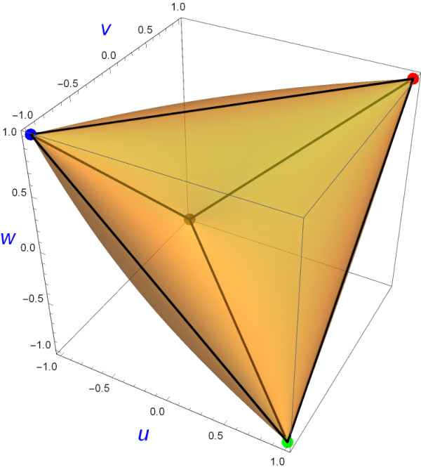
It is 33-dimensional and hence can be visualized, see Figure 4. All possible ground states lie at the boundary of 𝒢{\mathcal{G}}. This boundary consists of all Gram matrices GG with rank​(G)≤2\mbox{rank}(G)\leq 2 hence the ground states are 11- or 22-dimensional (Ising states or co-planar states). They can be divided into three classes:

  1. I

    The four special extremal points

    A0\displaystyle A_{0} =\displaystyle= [1,1,1],\displaystyle[1,1,1], (49)
    A1\displaystyle A_{1} =\displaystyle= [−1,−1,1],\displaystyle[-1,-1,1], (50)
    A2\displaystyle A_{2} =\displaystyle= [−1,1,−1],\displaystyle[-1,1,-1], (51)
    A3\displaystyle A_{3} =\displaystyle= [1,−1,−1],\displaystyle[1,-1,-1], (52)

    corresponding to the Ising matrices considered in section II.2.3. They correspond to the 2N−1=42^{N-1}=4 different Ising states due to rotational and/or reflectional equivalence.

  2. II

    A 22-dimensional manifold of extremal points defined by

    M\displaystyle M =\displaystyle= {[u,v,w]|−1<u,v,w<1,det[u,v,w]=0}.\displaystyle\{[u,v,w]\left|-1<u,v,w<1,\,\det[u,v,w]=0\right.\}.

    The corresponding ground states are co-planar.

  3. III

    Six open intervals joining all pairs of extremal points of type I:

    A0,A3¯\displaystyle\overline{A_{0},A_{3}} =\displaystyle= {[1,x,x]|−1<x<1},\displaystyle\{\,[1,x,x]\,|\,-1<x<1\,\}, (54)
    A0,A2¯\displaystyle\overline{A_{0},A_{2}} =\displaystyle= {[x,1,x]|−1<x<1},\displaystyle\{\,[x,1,x]\,|\,-1<x<1\,\}, (55)
    A0,A1¯\displaystyle\overline{A_{0},A_{1}} =\displaystyle= {[x,x,1]|−1<x<1},\displaystyle\{\,[x,x,1]\,|\,-1<x<1\,\}, (56)
    A2,A3¯\displaystyle\overline{A_{2},A_{3}} =\displaystyle= {[x,−x,−1]|−1<x<1},\displaystyle\{\,[x,-x,-1]\,|\,-1<x<1\,\}, (57)
    A1,A3¯\displaystyle\overline{A_{1},A_{3}} =\displaystyle= {[x,−1,−x]|−1<x<1},\displaystyle\{\,[x,-1,-x]\,|\,-1<x<1\,\}, (58)
    A1,A2¯\displaystyle\overline{A_{1},A_{2}} =\displaystyle= {[−1,x,−x]|−1<x<1}.\displaystyle\{\,[-1,x,-x]\,|\,-1<x<1\,\}\;. (59)

    The corresponding ground states are the special co-planar states such that two spins are parallel or anti-parallel.
Refer to caption
Figure 4: Plot of the convex Gram set 𝒢{\mathcal{G}} defined in (48) for N=3N=3 together with four extremal points corresponding to Ising states and the six faces generated by them. The points of 𝒢{\mathcal{G}} represent equivalence classes of spin configurations w. r. t. uniform rotations and/or reflections. Obviously, 𝒢{\mathcal{G}} has the full tetrahedral symmetry.

The closed faces of 𝒢{\mathcal{G}}, except the trivial ones ∅\emptyset and 𝒢{\mathcal{G}}, are the extremal points of the classes I and II and the six faces obtained by adding the end points to the six open intervals of class III. The manifold of class II consists of four connected parts divided by the six intervals of class III. Interestingly, these intervals fit smoothly into the manifold such that the union of the points of classes II and III again forms a manifold. This can be seen by simultaneously solving the equations det[u,v,w]=0\det\,[u,v,w]=0 and ∇det[u,v,w]=𝟎\nabla\det\,[u,v,w]={\mathbf{0}}. The only solutions are the four extremal points A0,A1,A2,A3A_{0},A_{1},A_{2},A_{3} of class I. This implies that the variety defined by det[u,v,w]=0\det\,[u,v,w]=0, if restricted to 𝒢{\mathcal{G}}, becomes a smooth two-dimensional manifold if the four points A0,A1,A2,A3A_{0},A_{1},A_{2},A_{3} are excluded.
Recall from section II.2 that the group 𝖲𝗒𝗆{\sf Sym} of symmetries of 𝒢{\mathcal{G}} is of order N!​ 2N−1N!\,2^{N-1} which equals 2424 for N=3N=3. Obviously, for the spin triangle 𝖲𝗒𝗆{\sf Sym} can be identified with the tetrahedral group ThT_{h} including reflections. Each transformation γ∈𝖲𝗒𝗆\gamma\in{\sf Sym} induces a permutation of the four extremal points A0,A1,A2,A3A_{0},A_{1},A_{2},A_{3}; and vice versa, every such permutation is induced by a unique symmetry γ∈𝖲𝗒𝗆\gamma\in{\sf Sym}. This illustrates the well-known isomorphism Th≅S4T_{h}\cong S_{4}. The use of symmetries simplifies the following investigations of ground states.
As remarked above the variety det[u,v,w]=0\det\,[u,v,w]=0 has exactly the four singular points A0,A1,A2,A3A_{0},A_{1},A_{2},A_{3}. Due to the symmetries of 𝒢{\mathcal{G}} it suffices to consider one of these singular points, say, A0=[1,1,1]A_{0}=[1,1,1] corresponding to the Ising state ↑↑↑\uparrow\uparrow\uparrow. In the infinitesimal neighbourhood of A0A_{0} the variety det[u,v,w]=0\det\,[u,v,w]=0 assumes the form of a circular cone C0C_{0}. This can be seen, e. g. , by expanding det[u,v,w]\det\,[u,v,w] at A0A_{0} up to second order. The set of affine functionals 𝒥:𝒢⟶ℝ{\mathcal{J}}:{\mathcal{G}}\longrightarrow{\mathbb{R}} defined by 𝒥⁡(G)≡Tr​(G​𝕁)=(u,v,w)⋅𝐉{\mathcal{J}}(G)\equiv\mbox{Tr}(G\,{\mathbb{J}})=(u,v,w)\cdot{\mathbf{J}} that assume their minimal value at A0A_{0} can be identified with the dual cone C0′C_{0}^{\prime} of C0C_{0}. Physically, this dual cone corresponds to the set of “ferromagnetic Hamiltonians" that have ground states of the form ↑↑↑\uparrow\uparrow\uparrow. In terms of the vectors 𝐉=(J1,J2,J3){\mathbf{J}}=(J_{1},J_{2},J_{3}) this “ferromagnetic cone" C0′C_{0}^{\prime} can be characterized by

𝐉⋅(1,1,1)=J1+J2+J3≤−‖𝐉‖.{\mathbf{J}}\cdot(1,1,1)=J_{1}+J_{2}+J_{3}\leq-||{\mathbf{J}}||\;. (60)

Note that C0′C_{0}^{\prime} is larger than the octant defined by J1,J2,J3≤0J_{1},J_{2},J_{3}\leq 0 , where the ferromagnetic nature of the Hamiltonian is self-evident.
According to the tetrahedral symmetry of 𝒢{\mathcal{G}} these results can be immediately transferred to the other extremal points A1,A2,A3A_{1},A_{2},A_{3}. For example, if 𝐄i{\mathbf{E}}_{i} denote the four vectors with the coordinates (w,v,u)(w,v,u) of the extremal points Ai,i=0,1,2,3A_{i},\,i=0,1,2,3, then the equations for the corresponding cones Ci′C_{i}^{\prime} that generalize (60) read:

𝐉⋅𝐄i≤−||𝐉||,i=0,1,2,3.{\mathbf{J}}\cdot{\mathbf{E}}_{i}\leq-||{\mathbf{J}}||,\;i=0,1,2,3\;. (61)

If 𝐉{\mathbf{J}} does not satisfy either of the four conditions (61) then its ground states will be co-planar and correspond to a point [u,v,w][u,v,w] of the manifold MM of class II considered above. The map from ground states to Hamiltonians [u,v,w]↦(J1,J2,J3)[u,v,w]\mapsto(J_{1},J_{2},J_{3}) can be easily determined: 𝐉{\mathbf{J}} can be chosen proportional to the gradient of 𝒟≡det[u,v,w]{\mathcal{D}}\equiv\det[u,v,w] w. r. t. the three variables u,v,wu,v,w:

J1\displaystyle J_{1} =\displaystyle= μ​∂𝒟∂w=2​μ​(u​v−w),\displaystyle\mu\frac{\partial{\mathcal{D}}}{\partial w}=2\mu(uv-w), (62)
J2\displaystyle J_{2} =\displaystyle= μ​∂𝒟∂v=2​μ​(w​u−v),\displaystyle\mu\frac{\partial{\mathcal{D}}}{\partial v}=2\mu(wu-v), (63)
J3\displaystyle J_{3} =\displaystyle= μ​∂𝒟∂u=2​μ​(v​w−u).\displaystyle\mu\frac{\partial{\mathcal{D}}}{\partial u}=2\mu(vw-u)\;. (64)

The converse is also straightforward: The solution of the system of equations (62),(63),(64) together with 𝒟=0{\mathcal{D}}=0 for the unknowns u,v,w,μu,v,w,\mu reads:

u\displaystyle u =\displaystyle= J12​J2​(J22J32−1)−J22​J1,\displaystyle\frac{{J_{1}}}{2{J_{2}}}\left(\frac{{J_{2}}^{2}}{{J_{3}}^{2}}-1\right)-\frac{{J_{2}}}{2{J_{1}}}, (65)
v\displaystyle v =\displaystyle= J12​J3​(J32J22−1)−J32​J1,\displaystyle\frac{{J_{1}}}{2{J_{3}}}\left(\frac{{J_{3}}^{2}}{{J_{2}}^{2}}-1\right)-\frac{{J_{3}}}{2{J_{1}}}, (66)
w\displaystyle w =\displaystyle= J22​J3​(J32J12−1)−J32​J2,\displaystyle\frac{{J_{2}}}{2{J_{3}}}\left(\frac{{J_{3}}^{2}}{{J_{1}}^{2}}-1\right)-\frac{{J_{3}}}{2{J_{2}}}, (67)
μ\displaystyle\mu =\displaystyle= −2​J13​J23​J33J14​(J22−J32)2−2​J12​J22​J32​(J22+J32)+J24​J34.\displaystyle\scriptstyle\frac{-2{J_{1}}^{3}{J_{2}}^{3}{J_{3}}^{3}}{{J_{1}}^{4}\left({J_{2}}^{2}-{J_{3}}^{2}\right)^{2}-2{J_{1}}^{2}{J_{2}}^{2}{J_{3}}^{2}\left({J_{2}}^{2}+{J_{3}}^{2}\right)+{J_{2}}^{4}{J_{3}}^{4}}\;. (68)

We will provide an example. Assume a Hamiltonian with J1=1,J2=−2,J3=−1J_{1}=1,\,J_{2}=-2,\,J_{3}=-1. One checks that the four conditions (61) are not satisfied and hence this Hamiltonian does not have an Ising ground state. Inserting the coupling constants into (65) – (68) yields u=14,v=78,w=−14,μ=1615u=\frac{1}{4},\,v=\frac{7}{8},\,w=-\frac{1}{4},\,\mu=\frac{16}{15} and a ground state energy of Em​i​n=J1​w+J2​v+J2​u=−94E_{min}=J_{1}\,w+J_{2}\,v+J_{2}\,u=-\frac{9}{4}. A possible ground state is hence 𝐬1=(1,0),𝐬2=(u,1−u2)=(14,154),𝐬3=(v,−1−v2)=(78,−158){\mathbf{s}}_{1}=(1,0),\,{\mathbf{s}}_{2}=(u,\sqrt{1-u^{2}})=\left(\frac{1}{4},\frac{\sqrt{15}}{4}\right),\,{\mathbf{s}}_{3}=(v,-\sqrt{1-v^{2}})=\left(\frac{7}{8},-\frac{\sqrt{15}}{8}\right). Note that the choice 𝐬3=(v,+1−v2){\mathbf{s}}_{3}=(v,+\sqrt{1-v^{2}}) would not give the correct value of 𝐬2⋅𝐬3=w=−14{\mathbf{s}}_{2}\cdot{\mathbf{s}}_{3}=w=-\frac{1}{4}. We will also check the SSE (4):

𝕁​𝐬\displaystyle{\mathbbm{J}}\,{\mathbf{s}} =\displaystyle= (0−12−1−12012−1120)​(101415478−158)\displaystyle\left(\begin{array}[]{ccc}0&-\frac{1}{2}&-1\\ -\frac{1}{2}&0&\frac{1}{2}\\ -1&\frac{1}{2}&0\\ \end{array}\right)\left(\begin{array}[]{cc}1&0\\ \frac{1}{4}&\frac{\sqrt{15}}{4}\\ \frac{7}{8}&-\frac{\sqrt{15}}{8}\\ \end{array}\right)
=\displaystyle= (−10−116−1516−78158)\displaystyle\left(\begin{array}[]{cc}-1&0\\ -\frac{1}{16}&-\frac{\sqrt{15}}{16}\\ -\frac{7}{8}&\frac{\sqrt{15}}{8}\\ \end{array}\right)
=\displaystyle= (−1000−14000−1)​(101415478−158).\displaystyle\left(\begin{array}[]{ccc}-1&0&0\\ 0&-\frac{1}{4}&0\\ 0&0&-1\\ \end{array}\right)\left(\begin{array}[]{cc}1&0\\ \frac{1}{4}&\frac{\sqrt{15}}{4}\\ \frac{7}{8}&-\frac{\sqrt{15}}{8}\\ \end{array}\right).

The negative mean value of the Lagrange parameters −κ¯=−34-\overline{\kappa}=-\frac{3}{4} is also the lowest eigenvalue jm​i​nj_{min} of the dressed 𝕁{\mathbbm{J}}-matrix in the ground state gauge

𝕁⁡(𝝀)=(14−12−1−12−1212−11214){\mathbbm{J}}({\boldsymbol{\lambda}})=\left(\begin{array}[]{ccc}\frac{1}{4}&-\frac{1}{2}&-1\\ -\frac{1}{2}&-\frac{1}{2}&\frac{1}{2}\\ -1&\frac{1}{2}&\frac{1}{4}\\ \end{array}\right) (87)

with two-fold degeneracy. This complies with Em​i​n=N​jm​i​n=3​(−34)=−94E_{min}=N\,j_{min}=3\,(-\frac{3}{4})=-\frac{9}{4}.

Refer to caption
Figure 5: The phase diagram of the set of spin coupling coefficients 𝐉=(J1,J2,J3){\mathbf{J}}=(J_{1},J_{2},J_{3}) restricted to the unit sphere. The four colored spherical shells correspond to systems that have Ising ground states of the kind Ai,i=0,1,2,3A_{i},\;i=0,1,2,3. The six common points (black dots) correspond to degenerate ground states (54) to (59). The area between the spherical shells corresponds to systems with co-planar ground states parametrized by the points of the manifold MM defined in ().

Summarizing, we can divide the unit sphere of the 𝐉{\mathbf{J}}-space into various parts, see figure 5. First, we have four closed spherical shells 𝒵i{\mathcal{Z}}_{i} that span the cones Ci′C_{i}^{\prime} considered above and belong to the four Ising ground states Ai,i=0,1,2,3A_{i},\;i=0,1,2,3. It turns out that each shell has three common points with the other three shells. The resulting number of 66 points in 𝐉{\mathbf{J}}-space corresponds to the 66 degenerate ground states of class III. The remaining part of the unit sphere not belonging to any 𝒵i{\mathcal{Z}}_{i} represents all normal directions of the manifold MM of class II. Together with MM it has four connected components.

In the following we consider four typical positions of 𝐉{\mathbf{J}} and the corresponding types of ground states. Let 𝐉=(6,−12,−14){\mathbf{J}}=(6,-12,-14); since J1+J2+J3=−20<−376=−‖𝐉‖J_{1}+J_{2}+J_{3}=-20<-\sqrt{376}=-||{\mathbf{J}}||, it follows that 𝐉{\mathbf{J}} lies in the interior of the ferromagnetic cone. W. r. t. the Ising state ↑↑↑\uparrow\uparrow\uparrow the ground state gauge 𝕁⁡(𝝀){\mathbb{J}}({\boldsymbol{\lambda}}) assumes the form

𝕁⁡(𝝀)=(193−7−6−7−833−63−113),{\mathbb{J}}({\boldsymbol{\lambda}})=\left(\begin{array}[]{ccc}\frac{19}{3}&-7&-6\\ -7&-\frac{8}{3}&3\\ -6&3&-\frac{11}{3}\\ \end{array}\right)\;, (88)

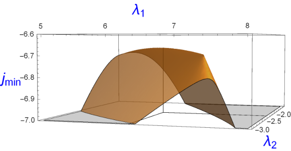
and its lowest eigenvalue ȷ^m​i​n=−203\hat{\jmath}_{min}=-\frac{20}{3} is non-degenerate with eigenvector (1,1,1)(1,1,1). Accordingly, at the point 𝝀=(193,−83){\boldsymbol{\lambda}}=(\frac{19}{3},-\frac{8}{3}) the function jm​i​n​(𝝀)j_{min}({\boldsymbol{\lambda}}) has a smooth maximum, see Figure 6.

Refer to caption
Figure 6: The minimal eigenvalue jm​i​n​(λ1,λ2)j_{min}(\lambda_{1},\lambda_{2}) of 𝕁⁡(λ1,λ2){\mathbb{J}}(\lambda_{1},\lambda_{2}), where J1=3,J2=−6,J3=−7J_{1}=3,\,J_{2}=-6,\,J_{3}=-7. At the point λ1=193,λ2=−83\lambda_{1}=\frac{19}{3},\,\lambda_{2}=-\frac{8}{3} the function jm​i​nj_{min} has a smooth maximum assuming the value ȷ^m​i​n=−203\widehat{\jmath}_{min}=-\frac{20}{3} corresponding to an Ising ground state ↑↑↑\uparrow\uparrow\uparrow.

If we increase J1J_{1} of the preceding example from the value 66 to 8413=6.461538¯\frac{84}{13}=6.\overline{461538}, 𝐉{\mathbf{J}} moves to the boundary of the ferromagnetic cone since J1+J2+J3=−25413=−‖𝐉‖J_{1}+J_{2}+J_{3}=-\frac{254}{13}=-||{\mathbf{J}}||. The plane perpendicular to 𝐉{\mathbf{J}} will now be tangent to the manifold MM of class II at the extremal point A0A_{0}. The ground state gauge w. r. t. ↑↑↑\uparrow\uparrow\uparrow assumes the form

Refer to caption
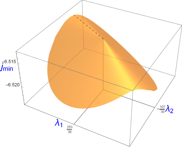
Figure 7: The minimal eigenvalue jm​i​n​(λ1,λ2)j_{min}(\lambda_{1},\lambda_{2}) of 𝕁⁡(λ1,λ2){\mathbb{J}}(\lambda_{1},\lambda_{2}), where J1=−7,J2=−6,J3=4213J_{1}=-7,\,J_{2}=-6,\,J_{3}=\frac{42}{13}. At the point λ1=25339,λ2=−10739\lambda_{1}=\frac{253}{39},\,\lambda_{2}=-\frac{107}{39} the function jm​i​nj_{min} assumes its maximal value ȷ^m​i​n=−25439\widehat{\jmath}_{min}=-\frac{254}{39}. At this point the function has a tangent cone with a horizontal direction (dashed line) at the angle φ=π−arctan⁡713\varphi=\pi-\arctan\frac{7}{13}.
𝕁⁡(𝝀)=(25339−7−6−7−107394213−64213−14639),{\mathbb{J}}({\boldsymbol{\lambda}})=\left(\begin{array}[]{ccc}\frac{253}{39}&-7&-6\\ -7&-\frac{107}{39}&\frac{42}{13}\\ -6&\frac{42}{13}&-\frac{146}{39}\\ \end{array}\right)\;, (89)

and its lowest eigenvalue ȷ^m​i​n=−25439\hat{\jmath}_{min}=-\frac{254}{39} becomes two-fold degenerate. The corresponding eigenspace spanned by (6/13,0,1)(6/13,0,1) and (7/13,1,0)(7/13,1,0) is still elliptic since the solution Δ\Delta of the system of equations corresponding to (30) has the eigenvalues 2,02,0. But only one eigenvector exists that gives rise to a spin configuration, namely the sum of the above two eigenvectors which again corresponds to ↑↑↑\uparrow\uparrow\uparrow. This is the example where the eigenspace of 𝕁⁡(𝝀){\mathbb{J}}({\boldsymbol{\lambda}}) is elliptic but not completely elliptic, that was announced on p. 2. At its maximum the function jm​i​n​(λ1,λ2)j_{min}(\lambda_{1},\lambda_{2}) is not smooth but has a tangent cone with a horizontal direction, see figure 7.

Refer to caption
Figure 8: The minimal eigenvalue jm​i​n​(λ1,λ2)j_{min}(\lambda_{1},\lambda_{2}) of 𝕁⁡(λ1,λ2){\mathbb{J}}(\lambda_{1},\lambda_{2}), where J1=1,J2=J3=−2J_{1}=1,\,J_{2}=J_{3}=-\sqrt{2}. At the point λ1=λ2=−1/3\lambda_{1}=\lambda_{2}=-1/3 the function jm​i​nj_{min} has a maximum with the value ȷ^m​i​n=−4/3\widehat{\jmath}_{min}=-4/3 and its graph assumes the form of a circular cone in the infinitesimal neighbourhood of the maximum.

Next we choose an example where 𝐉{\mathbf{J}} assumes its minimum at an extremal point belonging to the manifold MM of class II, see above, namely J1=J2=−2​2,J3=2J_{1}=J_{2}=-2\sqrt{2},\,J_{3}=2. The ground state(s) can be determined by using (65) – (67) which yields u=0,v=w=12u=0,\,v=w=\frac{1}{\sqrt{2}} and a ground state energy Em​i​n=−4E_{min}=-4. The corresponding Gram matrix [u,v,w][u,v,w] is, e. g. , realized by the spin configuration 𝐬1=(1,0),𝐬2=(0,1),𝐬3=(12,12){\mathbf{s}}_{1}=(1,0),\;{\mathbf{s}}_{2}=(0,1),\;{\mathbf{s}}_{3}=(\frac{1}{\sqrt{2}},\frac{1}{\sqrt{2}}). W. r. t. this configuration the dressed 𝕁{\mathbb{J}} matrix in the ground state gauge is obtained as:

𝕁⁡(𝝀)=(−131−21−13−2−2−223).{\mathbb{J}}({\boldsymbol{\lambda}})=\left(\begin{array}[]{ccc}-\frac{1}{3}&1&-\sqrt{2}\\ 1&-\frac{1}{3}&-\sqrt{2}\\ -\sqrt{2}&-\sqrt{2}&\frac{2}{3}\\ \end{array}\right). (90)

It has a doubly degenerate lowest eigenvalue ȷ^m​i​n=−43=13​Em​i​n{\hat{\jmath}}_{min}=-\frac{4}{3}=\frac{1}{3}E_{min} with an eigenspace spanned by the vectors 𝐞1=(2,0,1){\mathbf{e}}_{1}=(\sqrt{2},0,1) and 𝐞2=(−1,1,0){\mathbf{e}}_{2}=(-1,1,0). At its maximum the function jm​i​n​(λ1,λ2)j_{min}(\lambda_{1},\lambda_{2}) is not smooth but has a circular tangent cone, see figure 8.

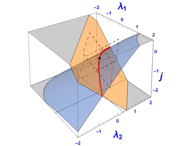
Finally we remark that the six cases of 𝐉=(±1,0,0){\mathbf{J}}=(\pm 1,0,0) and permutations correspond to disjoint systems where two spins are (anti)ferromagnetically coupled and the third spin is uncoupled. The ground state is hence a degenerate configuration where two spins are (anti)parallel and the third spin is arbitrary. These are the six cases (54) to (59). As an example we show the graph of jm​i​n​(λ1,λ2)j_{min}(\lambda_{1},\lambda_{2}) for the case of 𝐉=(0,0,1){\mathbf{J}}=(0,0,1), see Figure 9. At the maximum of jm​i​n​(λ1,λ2)j_{min}(\lambda_{1},\lambda_{2}) the elliptic tangent cone degenerates into a wedge.
Refer to caption
Figure 9: The minimal eigenvalue jm​i​n​(λ1,λ2)j_{min}(\lambda_{1},\lambda_{2}) of 𝕁⁡(λ1,λ2){\mathbb{J}}(\lambda_{1},\lambda_{2}), where J1=J2=0,J3=1J_{1}=J_{2}=0,\,J_{3}=1. jm​i​n​(λ1,λ2)j_{min}(\lambda_{1},\lambda_{2}) is the minimum of two smooth eigenvalue functions j1​(λ1,λ2)j_{1}(\lambda_{1},\lambda_{2}) and j2​(λ1,λ2)j_{2}(\lambda_{1},\lambda_{2}). The intersection between the graphs of j1​(λ1,λ2)j_{1}(\lambda_{1},\lambda_{2}) and j2​(λ1,λ2)j_{2}(\lambda_{1},\lambda_{2}) is shown as a red curve. At the point λ1=λ2=13\lambda_{1}=\lambda_{2}=\frac{1}{3} the function jm​i​nj_{min} assumes its maximal value ȷ^m​i​n=−23\widehat{\jmath}_{min}=-\frac{2}{3} (black dot). At this point the tangent cone degenerates into a wedge generated by the two tangent planes at j1​(λ1,λ2)j_{1}(\lambda_{1},\lambda_{2}) and j2​(λ1,λ2)j_{2}(\lambda_{1},\lambda_{2}) with a horizontal intersection (dashed lines).

IV Summary and Outlook

In this paper we have started the investigation of the convex set 𝒢{\mathcal{G}} of Gram matrices of NN spins. This leads to a slightly different view on the ground state problem: The points of 𝒢{\mathcal{G}} are O⁡(M)O(M)-equivalence classes of spin configurations and each Heisenberg Hamiltonian is an affine functional defined on 𝒢{\mathcal{G}} such that its minimal energy value is assumed at a face of 𝒢{\mathcal{G}}. If the face is an extremal point, the ground state is essentially unique; but if it consists of more than one point (or, equivalently, has a dimension >0>0) we encounter the effect of additional degeneracy that is familiar from many examples. Hence we are lead to the general problem to classifying and characterizing the faces of 𝒢{\mathcal{G}}, a problem that we have to defer to subsequent papers. An equivalent problem would be the classification of completely elliptic subspaces of ℝN{\mathbbm{R}}^{N}. In the present paper we have found some partial results on the subset of extremal points corresponding to Ising states and calculated the complete symmetry group of 𝒢{\mathcal{G}}. The latter is also of avail for practical purposes.

The second part of the paper was devoted to the ground state problem of the general spin triangle, where 𝒢{\mathcal{G}} can be visualized as a subset of ℝ3{\mathbbm{R}}^{3} and its structure can be completely clarified. It was also possible in this case to visualize for typical cases the Lagrange variety in the neighborhood of vertical points corresponding to ground state(s) of suitable Hamiltonians. As we have shown, there exists an algorithm to calculate the ground state(s) for any given Heisenberg Hamiltonian, but it is pretty obvious that this cannot be generalized to larger NN.

Appendix A Elliptic subspaces

Recall that a “completely elliptic subspace" (CES) SS of ℝN{\mathbbm{R}}^{N} is defined by the existence of an N×MN\times M-matrix WW such that its MM columns form a basis of S{S} and its NN rows are unit vectors. Alternatively, a CES S{S} is characterized by the property that for any N×MN\times M-matrix WW such that its MM columns form a basis of S{S} the NN rows will lie an a non-degenerate N−N-dimensional ellipsoid. It will be instructive to determine the completely elliptic subspaces for simple examples. As an obvious general result we note that permutations of coordinates and partial reflections ρ𝒯\rho_{\mathcal{T}}, see(27), map the class of CES onto itself. In this paper we have determined the CES of ℝ3{\mathbbm{R}}^{3}.

A.1 Complete elliptic subspaces of ℝ3{\mathbbm{R}}^{3}

Obviously, there exist exactly four one-dimensional CES Lμ,μ=0,…,3L_{\mu},\mu=0,\ldots,3 of ℝ3{\mathbbm{R}}^{3} spanned by the vectors (1,1,1),(−1,1,1),(1,−1,1),(1,1,−1)(1,1,1),\;(-1,1,1),\;(1,-1,1),\;(1,1,-1) , resp. . The LμL_{\mu} are connected by partial reflections, see above, and can be visualized by the four space diagonals of the cube.

Refer to caption
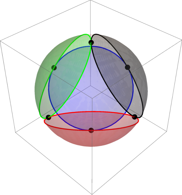
Figure 10: The set of normal vectors C​E​NCEN of completely elliptic two-dimensional subspaces of ℝ3{\mathbbm{R}}^{3}. A completely elliptic subspace hosts two-dimensional spin configurations. In this case C​E​NCEN is the union of the open interior of the triangles bounded by the four (colored) great circles perpendicular to the four (colored) space diagonals and the set of its vertices.

Two-dimensional subspaces of ℝ3{\mathbbm{R}}^{3} are conveniently represented by their normal vectors which are unique up to a sign. Hence they should rather be considered as elements of the projective plane ℙ2​(ℝ){\mathbbm{P}}^{2}({\mathbbm{R}}). Let C​E​N⊂ℙ2​(ℝ)CEN\subset{\mathbbm{P}}^{2}({\mathbbm{R}}) denote the set of normal vectors of CES. Any two-dimensional subspace S{S} containing one of the lines LμL_{\mu} is an elliptic subspace, although not a completely one. But it can be obtained as a limit of CES such that the ellipses spanned by the rows of the corresponding WW degenerate into a pair of parallel lines. It follows that the normal vectors of such two-dimensional subspaces S{S} run through the great circle CμC_{\mu} of the unit sphere perpendicular to LμL_{\mu}. Hence the four great circles Cμ,μ=0,…,3C_{\mu},\mu=0,\ldots,3 form the boundary of the set C​E​NCEN of normals of CES. These great circles divide the unit sphere into 88 triangles and 66 squares and hence define a structure that could be called the “projective cuboctahedron", see Figure 10. Obviously, the partial reflections and permutations operate as symmetries of the projective cuboctahedron. It remains to decide whether the C​E​NCEN is generated by the open interior of the triangles or of the squares. To this end we consider the matrix

W=(−1232−12−3210),W=\left(\begin{array}[]{cc}-\frac{1}{2}&\frac{\sqrt{3}}{2}\\ -\frac{1}{2}&-\frac{\sqrt{3}}{2}\\ 1&0\\ \end{array}\right)\;, (91)

the columns of which span a CES with normal vector 𝐰=(13,13,13){\mathbf{w}}=(\frac{1}{\sqrt{3}},\frac{1}{\sqrt{3}},\frac{1}{\sqrt{3}}). Since 𝐰{\mathbf{w}} lies inside the triangle of the projective cuboctahedron bounded by C1,C2,C3C_{1},\,C_{2},\,C_{3} we conclude that C​E​NCEN is generated by the four open interiors of the triangles (there are eight triangles but they have to be pair-wise identified due to the undetermined sign of the normal vectors), see Figure 10. Contrary to the first sight C​E​NCEN is not an open subset of ℙ2​(ℝ){\mathbbm{P}}^{2}({\mathbbm{R}}) since the vertices of the triangles also belong to it.

It will be instructive to re-derive the above characterization of the CES of ℝ3{\mathbbm{R}}^{3} by means of the Lagrange variety approach. Let S⊂ℝ3S\subset{\mathbbm{R}}^{3} be CES of dimension 22 and 𝐰{\mathbf{w}} be a unit vector normal to SS. Further, let PP be the projector onto 𝐰{\mathbf{w}}, i. e., Pi​j=wi​wjP_{i\,j}=w_{i}\,w_{j}. Since, by construction, the support of PP is orthogonal to SS, we may set P=𝕁⁡(𝜿ˇ)P={\mathbbm{J}}(\check{\boldsymbol{\kappa}}) such that the Gram matrix GG of a two-dimensional ground state 𝐬{\mathbf{s}} of 𝕁{\mathbbm{J}} lives on SS, see Theorem 2, and 𝜿ˇ\check{\boldsymbol{\kappa}} are the Lagrange parameters w. r. t. the ground state 𝐬{\mathbf{s}}. We expand the determinant 𝒟=det𝕁⁡(𝜿){\mathcal{D}}=\det{\mathbbm{J}}({\boldsymbol{\kappa}}) up to second order w. r. t. the parameters 𝐱≡𝜿−𝜿ˇ{\mathbf{x}}\equiv{\boldsymbol{\kappa}}-\check{\boldsymbol{\kappa}} and obtain

𝒟=12​⟨𝐱​|M|​𝐱⟩+O⁡(‖x‖3),{\mathcal{D}}=\frac{1}{2}\langle{\mathbf{x}}\left|M\right|{\mathbf{x}}\rangle+O(||x||^{3})\;, (92)

where

M=(0w32w22w320w12w22w120).M=\left(\begin{array}[]{ccc}0&w_{3}^{2}&w_{2}^{2}\\ w_{3}^{2}&0&w_{1}^{2}\\ w_{2}^{2}&w_{1}^{2}&0\\ \end{array}\right)\;. (93)

In the generic case, that is for detM≠0\det M\neq 0, ⟨𝐱​|M|​𝐱⟩=0\langle{\mathbf{x}}\left|M\right|{\mathbf{x}}\rangle=0 defines an elliptic double cone 𝒞{\mathcal{C}} that approximates the variety 𝒟=0{\mathcal{D}}=0 in the neighborhood of 𝐱=𝟎{\mathbf{x}}={\mathbf{0}}. For detM=0\det M=0 this cone degenerates into a wedge spanned by two planes, see Figure 9 for an example. According to Theorem 2,  SS is elliptic iff the cone 𝒞{\mathcal{C}} is vertical. An equivalent condition for verticality is that the plane 𝐞⟂{\mathbf{e}}^{\perp} perpendicular to 𝐞=(1,1,1){\mathbf{e}}=(1,1,1) supports 𝒞{\mathcal{C}}, which is satisfied if 𝐞⟂{\mathbf{e}}^{\perp} intersects 𝒞{\mathcal{C}} only at the origin. Hence we look for solutions of

0\displaystyle 0 =\displaystyle= (x1x2−x1−x2)⋅M⋅(x1x2−x1−x2)\displaystyle\left(\begin{array}[]{c}x_{1}\\ x_{2}\\ -x_{1}-x_{2}\\ \end{array}\right)\cdot M\cdot\left(\begin{array}[]{c}x_{1}\\ x_{2}\\ -x_{1}-x_{2}\\ \end{array}\right)
=\displaystyle= (x1x2)⋅(−2​w22−w12−w22+w32−w12−w22+w32−2​w12)⋅(x1x2)\displaystyle\scriptsize\left(\begin{array}[]{c}x_{1}\\ x_{2}\\ \end{array}\right)\cdot\left(\begin{array}[]{cc}-2w_{2}^{2}&-w_{1}^{2}-w_{2}^{2}+w_{3}^{2}\\ -w_{1}^{2}-w_{2}^{2}+w_{3}^{2}&-2w_{1}^{2}\\ \end{array}\right)\cdot\left(\begin{array}[]{c}x_{1}\\ x_{2}\\ \end{array}\right)
≡\displaystyle\equiv (x1x2)⋅A⋅(x1x2).\displaystyle\left(\begin{array}[]{c}x_{1}\\ x_{2}\\ \end{array}\right)\cdot A\cdot\left(\begin{array}[]{c}x_{1}\\ x_{2}\\ \end{array}\right)\;.

This equation has only the trivial solution x1=x2=0x_{1}=x_{2}=0 iff detA>0\det A>0. After some calculations we obtain

detA\displaystyle\det A =\displaystyle= −w14+2​(w22+w32)​w12−(w22−w32)2\displaystyle-w_{1}^{4}+2\left(w_{2}^{2}+w_{3}^{2}\right)w_{1}^{2}-\left(w_{2}^{2}-w_{3}^{2}\right)^{2} (114)
=\displaystyle= (w1+w2−w3)​(w1−w2+w3)\displaystyle(w_{1}+w_{2}-w_{3})(w_{1}-w_{2}+w_{3})
(−w1+w2+w3)​(w1+w2+w3).\displaystyle(-w_{1}+w_{2}+w_{3})(w_{1}+w_{2}+w_{3})\;. (115)

Hence detA>0\det A>0 describes the open interior of the four triangles bounded by the great circles C0,C1,C2,C3C_{0},\,C_{1},\,C_{2},\,C_{3} mentioned above and thus characterizes C​E​NCEN except for the vertices of the triangles. It is interesting to note that the polynomial (115) is a symmetric polynomial not only w. r. t. permutations but also w. r. t. the partial reflections ρ𝒯\rho_{\mathcal{T}}.

According to Theorem 2 we have the bijections Fac​(𝒢)↔𝔼↔C​E​S\mbox{\sf Fac}({\mathcal{G}})\leftrightarrow{\mathbb{E}}\leftrightarrow CES. It will be interesting to identify the bijection Fac​(𝒢)↔C​E​S\mbox{\sf Fac}({\mathcal{G}})\leftrightarrow CES for the general spin triangle. The interior of the four triangles that together generate C​E​NCEN corresponds to the four connected components of the manifold MM defined in () consisting of co-planar ground states. Each connected component of MM is enclosed by three line segments Ai,Aj¯\overline{A_{i},A_{j}} of the form (54) – (59) consisting of families of co-planar ground states with two spin vectors parallel or anti-parallel. Since these families generate the same CES they correspond to the three vertices of the above-mentioned triangles, resp., that connect each triangle to its three neighbors. Finally, as we have already seen, the great circles Cμ,μ=0,…,3C_{\mu},\mu=0,\ldots,3 correspond to Ising ground states and hence to the four extremal points Ai,i=0,1,2,3A_{i},\,i=0,1,2,3 defined in (49). Each great circle CμC_{\mu} touches three triangles of the projective cuboctahedron in the same way as each extremal point AiA_{i} touches three of the four connected components of MM.

Appendix B The group of symmetries of the Gram set

Recall that the Gram set 𝒢=𝒢N{\mathcal{G}}={\mathcal{G}}_{N} is an (N2){N\choose 2}-dimensional compact convex set. The group of affine bijections, or “symmetries", σ:𝒢⟶𝒢\sigma:{\mathcal{G}}\longrightarrow{\mathcal{G}} will preliminary be denoted by 𝖠𝗎𝗍{\sf Aut}. We have shown in section II.2 that permutations π\pi of NN spins and partial reflections ρ𝒯,𝒯⊂{1,…,N},\rho_{\mathcal{T}},\;{\mathcal{T}}\subset\{1,\ldots,N\},\, generate affine bijections of 𝒢{\mathcal{G}} via G↦Π⁡(G)=U​(π)−1​G​U​(π)G\mapsto\Pi(G)=U(\pi)^{-1}\,G\,U(\pi) and G↦𝖱𝒯​(G)=V⁡(ρ𝒯)​G​V​(ρ𝒯)G\mapsto{\sf R}_{\mathcal{T}}(G)=V(\rho_{\mathcal{T}})\,G\,V(\rho_{\mathcal{T}}). These special symmetries form subgroups 𝖯𝖾𝗋{\sf Per} and 𝖱𝖿{\sf Rf} of 𝖠𝗎𝗍{\sf Aut}. The finite subgroup of 𝖠𝗎𝗍{\sf Aut} generated by 𝖯𝖾𝗋{\sf Per} and 𝖱𝖿{\sf Rf} has been denoted by 𝖲𝗒𝗆{\sf Sym}. We note the following:

Lemma 4

𝖱𝖿{\sf Rf} is a normal subgroup of 𝖲𝗒𝗆{\sf Sym}.

Proof
It suffices to show that for all Π∈𝖯𝖾𝗋\Pi\in{\sf Per} and 𝒯⊂{1,…,N}{\mathcal{T}}\subset\{1,\ldots,N\} there exists a 𝒯′⊂{1,…,N}{\mathcal{T}}^{\prime}\subset\{1,\ldots,N\} such that Π​𝖱𝒯​Π−1=𝖱𝒯′\Pi\,{\sf R}_{\mathcal{T}}\,\Pi^{-1}={\sf R}_{{\mathcal{T}}^{\prime}}. This holds for 𝒯′≡{π(μ)|μ∈𝒯}{\mathcal{T}}^{\prime}\equiv\{\pi(\mu)\left|\mu\in{\mathcal{T}}\right.\} which implies V⁡(ρ𝒯′)=Uπ−1​V​(ρ𝒯)​UπV(\rho_{{\mathcal{T}}^{\prime}})=U_{\pi}^{-1}\,V(\rho_{\mathcal{T}})\,U_{\pi} and further

Π​𝖱𝒯​Π−1​(G)\displaystyle\Pi\,{\sf R}_{\mathcal{T}}\,\Pi^{-1}(G) =\displaystyle= Uπ−1​V​(ρ𝒯)​Uπ​G​Uπ−1​V​(ρ𝒯)​Uπ\displaystyle U_{\pi}^{-1}\,V({\rho_{\mathcal{T}}})\,U_{\pi}\,G\,U_{\pi}^{-1}\,V({\rho_{\mathcal{T}}})\,U_{\pi} (116)
=\displaystyle= V⁡(ρ𝒯′)​G​V​(ρ𝒯′)=𝖱𝒯′​(G).\displaystyle V({\rho_{{\mathcal{T}}^{\prime}}})\,G\,V({\rho_{{\mathcal{T}}^{\prime}}})={\sf R}_{{\mathcal{T}}^{\prime}}(G)\;.

□\Box

As the main result of this section we will prove that permutations and partial reflections already generate the group of all symmetries:

Theorem 4

𝖠𝗎𝗍{\sf Aut} = 𝖲𝗒𝗆{\sf Sym}.

The proof of this theorem will be split into a couple of lemmas.

Lemma 5

Every symmetry σ∈𝖠𝗎𝗍\sigma\in{\sf Aut} maps ℐ{\mathcal{I}} onto ℐ{\mathcal{I}}.

Proof
It is clear that σ∈𝖠𝗎𝗍\sigma\in{\sf Aut} maps extremal points of 𝒢{\mathcal{G}} onto extremal points. Ising matrices are exactly the extremal points G0G_{0} of 𝒢{\mathcal{G}} with rank ​G0=1\mbox{rank }G_{0}=1 and hence the closed faces of the form {G0}=𝖿𝖺𝖼⁡(S)\{G_{0}\}={\sf fac}(S) where the completely elliptic subspace SS is one-dimensional and thus S⟂S^{\perp} is (N−1)(N-1)-dimensional. Then the property rank ​G0=1\mbox{rank }G_{0}=1 can be cast into the language of affine geometry by the equivalent statement that the cone 𝒞⁡(G0){\mathcal{C}}(G_{0}) defined in Theorem 3 (iii) has the maximal dimension 12​N​(N−1)\frac{1}{2}N(N-1). Consequently this property is respected by symmetries σ∈𝖠𝗎𝗍\sigma\in{\sf Aut} that hence generate permutations of ℐ{\mathcal{I}}. □\Box

Lemma 5 immediately implies:

Lemma 6

The barycenter 𝟙N{\mathbbm{1}}_{N} of ℐ{\mathcal{I}} is a fixed point for all σ∈𝖠𝗎𝗍\sigma\in{\sf Aut}.

It will be convenient to replace 𝒢{\mathcal{G}} by the affinely isomorphic convex set 𝒢−𝟙N{\mathcal{G}}-{\mathbbm{1}}_{N}. Consequently, the symmetries σ∈𝖠𝗎𝗍\sigma\in{\sf Aut} leave the point 𝕆{\mathbbm{O}}, the barycenter of ℐ{\mathcal{I}}, fixed and hence can be considered as linear transformations of the linear space ℒ{\mathcal{L}} spanned by 𝒢{\mathcal{G}}. As a consequence in the remainder of this section we will usually make no difference between, say, AA and A^=A−𝟙\hat{A}=A-{\mathbbm{1}}.

Lemma 7

The linear span of ℐ{\mathcal{I}} is ℒ{\mathcal{L}}, the linear space of all symmetric N×NN\times N-matrices with vanishing diagonal and hence of dimension (N2){N\choose 2}.

Proof
We will prove this lemma by induction over NN. For N=2N=2 the two matrices A0^=(0110)\hat{A_{0}}=\left(\begin{array}[]{cc}0&1\\ 1&0\end{array}\right) and A0^=(0−1−10)\hat{A_{0}}=\left(\begin{array}[]{cc}0&-1\\ -1&0\end{array}\right) are linearly dependent and dimℒ=1\dim{\mathcal{L}}=1.

For the induction step N→N+1N\rightarrow N+1 we may assume that the linear span of ℐN{\mathcal{I}}_{N} is ℒN{\mathcal{L}}_{N} and dimℒN=(N2)\dim{\mathcal{L}}_{N}={N\choose 2}. The notation ℐN{\mathcal{I}}_{N} denoting the set of Ising matrices for NN spins must not be confused with the notation ℐk{\mathcal{I}}_{k} denoting sets of kk-Ising matrices introduced in section II.2.3. For each Ising state 𝐬{\mathbf{s}} of NN spins we obtain two Ising states 𝐬+{\mathbf{s}}+ and 𝐬−{\mathbf{s}}- of N+1N+1 spins by choosing 𝐬N+1=+1{\mathbf{s}}_{N+1}=+1 or −1-1, resp. . For the Ising matrices G^​(𝐬+)\hat{G}({\mathbf{s}}+) and G^​(𝐬−)\hat{G}({\mathbf{s}}-) this means that G^​(𝐬)\hat{G}({\mathbf{s}}) is augmented by a copy of its first row (column), or by a negative copy of its first row (column), except the marginal values G^​(𝐬±)1,N+1=G^​(𝐬±)N+1,1=±1\hat{G}({\mathbf{s}}\pm)_{1,N+1}=\hat{G}({\mathbf{s}}\pm)_{N+1,1}=\pm 1 and G^​(𝐬±)N+1,N+1=0\hat{G}({\mathbf{s}}\pm)_{N+1,N+1}=0. Let 𝐬{\mathbf{s}} run through a set INI_{N} of (N2){N\choose 2} Ising states such that the corresponding set {G^(𝐬)|𝐬∈IN}\{\hat{G}({\mathbf{s}})\left|{\mathbf{s}}\in I_{N}\right.\} forms a basis of ℒN{\mathcal{L}}_{N}. Then the set ℬ≡{12(G^(𝐬+)+G^(𝐬−))|𝐬∈IN}{\mathcal{B}}\equiv\{\frac{1}{2}\left(\hat{G}({\mathbf{s}}+)+\hat{G}({\mathbf{s}}-)\right)\left.\right|{\mathbf{s}}\in I_{N}\} consists of copies of the matrices in the above basis of ℒN{\mathcal{L}}_{N} augmented by zero rows/columns. Hence it is a linearly independent set in ℒN+1{\mathcal{L}}_{N+1}. Recall that the sum of all matrices in ℐN{\mathcal{I}}_{N} yields the zero matrix 𝕆{\mathbbm{O}}. It follows that the corresponding sum of (N+1)×(N+1)(N+1)\times(N+1)-matrices G^​(𝐬+)\hat{G}({\mathbf{s}}+), multiplied with 1|ℐN|\frac{1}{|{\mathcal{I}}_{N}|}, yields a matrix H=H(1)H=H^{(1)} with zero entries except HN+1,1=H1,N+1=1H_{N+1,1}=H_{1,N+1}=1. It follows that HH cannot be obtained as a linear combination of matrices from ℬ{\mathcal{B}}, hence ℬ∪{H}{\mathcal{B}}\cup\{H\} is still linearly independent. Let π=(1,μ)\pi=(1,\mu), the transposition swapping 11 and μ, 2≤μ≤N\mu,\;2\leq\mu\leq N. The corresponding symmetry H↦Π⁡(H)H\mapsto\Pi(H) swaps the first and the μ\mu-th row/column of GG. Hence the N−1N-1 resulting matrices H(μ)≡Π⁡(H)H^{(\mu)}\equiv\Pi(H), that are in the linear span of ℐN+1{\mathcal{I}}_{N+1}, have only zero entries except Π​(H)N+1,μ=Hμ,N+1=1\Pi(H)_{N+1,\mu}=H_{\mu,N+1}=1. The set 𝒜≡{H(μ)|μ=1,…,N}{\mathcal{A}}\equiv\{H^{(\mu)}|\mu=1,\ldots,N\} is hence linearly independent in ℒN+1{\mathcal{L}}_{N+1} and 𝒜∪ℬ{\mathcal{A}}\cup{\mathcal{B}} forms a basis of ℒN+1{\mathcal{L}}_{N+1} with (N2)+N=(N+12){N\choose 2}+N={N+1\choose 2} elements. □\Box

Lemma 8

If σ∈𝖠𝗎𝗍\sigma\in{\sf Aut} leaves all points of ℐ{\mathcal{I}} fixed then it is the identity.

Proof
This follows immediately from Lemma 7 since σ\sigma is a linear map and under the assumption of the lemma it leaves all points of ℒ{\mathcal{L}}, the linear span of ℐ{\mathcal{I}}, fixed. □\Box

It follows from Lemma 8 that a symmetry σ∈𝖠𝗎𝗍\sigma\in{\sf Aut} is completely determined by its action on ℐ{\mathcal{I}}. Indeed, for every other symmetry τ∈𝖠𝗎𝗍\tau\in{\sf Aut} that coincides with σ\sigma on ℐ{\mathcal{I}}, it follows that τ−1​σ\tau^{-1}\,\sigma leaves all points of ℐ{\mathcal{I}} fixed, and, by Lemma 8, σ=τ\sigma=\tau. This further implies that 𝖠𝗎𝗍{\sf Aut} is isomorphic to a subgroup of the group of permutations of ℐ{\mathcal{I}} and hence finite. Hence we have shown:

Lemma 9

𝖠𝗎𝗍{\sf Aut} is a finite group. Every symmetry σ∈𝖠𝗎𝗍\sigma\in{\sf Aut} is completely determined by its action on ℐ{\mathcal{I}}.

One easily proves that the subgroup 𝖲𝗒𝗆{\sf Sym} of 𝖠𝗎𝗍{\sf Aut} consists of orthogonal transformations w. r. t. the scalar product Tr ​A​B\mbox{Tr }A\,B, but the same property need not hold for the possibly larger group 𝖠𝗎𝗍{\sf Aut}. For this reason we define another Euclidean scalar product ≺|≻\prec\,|\,\succ on the linear space ℒ{\mathcal{L}} by averaging the former scalar product over the action of 𝖠𝗎𝗍{\sf Aut}:

≺A|B≻≡1|𝖠𝗎𝗍|​∑σ∈𝖠𝗎𝗍Tr ​(σ⁡(A^)​σ​(B^)).\prec A|B\succ\equiv\frac{1}{|{\sf Aut}|}\sum_{\sigma\in{\sf Aut}}\mbox{Tr }(\sigma(\hat{A})\,\sigma(\hat{B}))\;. (117)

At the r. h. s. of (117) we have made use of the matrix properties of the points of ℒ{\mathcal{L}} and consequently re-introduced the ^\hat{}\;-notation. It follows that all symmetries σ∈𝖠𝗎𝗍\sigma\in{\sf Aut} are ≺|≻\prec\,|\,\succ-orthogonal transformations, whereas the σ∈𝖲𝗒𝗆\sigma\in{\sf Sym} are additionally orthogonal transformations w. r. t. the former scalar product Tr ​A​B\mbox{Tr }A\,B. Nevertheless, the following holds:

Lemma 10

All distances between Ising matrices calculated in section II.2.3 have the same value also if calculated w. r. t. the scalar product ≺|≻\prec\,|\,\succ defined in (117).

Proof
First we show that the norm of Ising matrices is the same for both scalar products. This follows since σ⁡(𝜸)∈ℐ\sigma({\boldsymbol{\gamma}})\in{\mathcal{I}} for all 𝜸∈ℐ{\boldsymbol{\gamma}}\in{\mathcal{I}} and hence Tr ​(σ⁡(𝜸^)​σ​(𝜸^))=N⁡(N−1)\mbox{Tr }(\sigma(\hat{\boldsymbol{\gamma}})\,\sigma(\hat{\boldsymbol{\gamma}}))=N(N-1) for all σ∈𝖠𝗎𝗍\sigma\in{\sf Aut}. Therefore the averaging in (117) of the constant value yields ≺𝜸^|𝜸^≻=N⁡(N−1)\prec\hat{\boldsymbol{\gamma}}|\hat{\boldsymbol{\gamma}}\succ=N(N-1).

Next we consider the representation of the barycenter BkB_{k} of ℐk{\mathcal{I}}_{k}, see (35), that can be re-written as Bk=α​A0B_{k}=\alpha A_{0}. This representation is independent of the choice of the scalar product, but it is not clear whether BkB_{k} is the
≺|≻\prec\,|\,\succ-projection of all 𝜸∈ℐk{\boldsymbol{\gamma}}\in{\mathcal{I}}_{k} onto the line through A0A_{0}. Hence let Ck=β​A0C_{k}=\beta A_{0} be the ≺|≻\prec\,|\,\succ-projection of an arbitrary 𝜸∈ℐk{\boldsymbol{\gamma}}\in{\mathcal{I}}_{k} onto the line through A0A_{0} and let 𝜸′∈ℐk{\boldsymbol{\gamma}}^{\prime}\in{\mathcal{I}}_{k} be a different point. Then there exists a permutation π∈SN\pi\in S_{N} such that the corresponding symmetry Π\Pi maps 𝜸{\boldsymbol{\gamma}} onto 𝜸′{\boldsymbol{\gamma}}^{\prime} and leaves A0A_{0} fixed. Since Π\Pi is also a ≺|≻\prec\,|\,\succ-orthogonal transformation, 𝜸′{\boldsymbol{\gamma}}^{\prime} has the same ≺|≻\prec\,|\,\succ-projection onto the line through A0A_{0} as 𝜸{\boldsymbol{\gamma}}. Consequently all 𝜸∈ℐk{\boldsymbol{\gamma}}\in{\mathcal{I}}_{k} and hence also the barycenter BkB_{k} have the same projection Ck=β​A0C_{k}=\beta A_{0} onto the line through A0A_{0}. But BkB_{k} is already of the form Bk=α​A0B_{k}=\alpha A_{0} hence Bk=CkB_{k}=C_{k} and we have shown that the projection does not depend on the scalar product.

From this it follows immediately that (33) and (34) also hold for the new scalar product ≺|≻\prec\,|\,\succ. For the distances between arbitrary pairs of points in ℐk{\mathcal{I}}_{k} the analogous statement follows by application of the symmetries 𝖱𝒯{\sf R}_{\mathcal{T}} generated by partial reflections ρ𝒯\rho_{\mathcal{T}} that are isometries w. r. t. either scalar product. □\Box

Lemma 11

If a symmetry σ∈𝖠𝗎𝗍\sigma\in{\sf Aut} leaves A0A_{0} fixed then it maps the sets ℐk{\mathcal{I}}_{k} onto ℐk{\mathcal{I}}_{k} for all k=1,…,⌊N2⌋k=1,\ldots,\lfloor\frac{N}{2}\rfloor.

Proof
The lemma follows since, by (34), the sets ℐk{\mathcal{I}}_{k} are exactly the subsets of ℐ{\mathcal{I}} that have a constant distance 2​2​k​(N−k)2\,\sqrt{2\,k\,(N-k)} to A0A_{0} and since σ∈𝖠𝗎𝗍\sigma\in{\sf Aut} is an ≺|≻\prec\,|\,\succ-isometry. Note that also Lemma 10 is needed for insuring that the above distances are the same for both scalar products. □\Box

Lemma 12

If a symmetry σ∈𝖠𝗎𝗍\sigma\in{\sf Aut} leaves A0A_{0} and all Aμ∈ℐ1,μ=1,…,N,A_{\mu}\in{\mathcal{I}}_{1},\;\mu=1,\ldots,N, fixed then it is the identity.

Proof
By Lemma 11 the sets ℐk{\mathcal{I}}_{k} are left invariant by σ\sigma. It suffices to show that σ\sigma is the identity for all ℐk,k=2,…,⌊N2⌋{\mathcal{I}}_{k},\;k=2,\ldots,\lfloor\frac{N}{2}\rfloor since it is completely determined by its action on ℐ{\mathcal{I}}, see Lemma 9. We will prove the claim by induction over kk and start with k=2k=2. Since we will make use of the matrix properties of the points of ℐ{\mathcal{I}} it will be appropriate to distinguish between, say, AA and A^=A−𝟙\hat{A}=A-{\mathbbm{1}} and to undo the translation 𝒢↦𝒢−𝟙{\mathcal{G}}\mapsto{\mathcal{G}}-{\mathbbm{1}} for the remainder of this proof.

Let A{μ,ν}, 1≤μ<ν≤NA_{\{\mu,\nu\}},\;1\leq\mu<\nu\leq N be an arbitrary element of ℐ2{\mathcal{I}}_{2}. Recall that A{μ,ν}A_{\{\mu,\nu\}} is the Gram matrix of an Ising spin configuration 𝐬{\mathbf{s}} where, say, all spins are ↑\uparrow except 𝐬μ=𝐬ν=↓{\mathbf{s}}_{\mu}={\mathbf{s}}_{\nu}=\downarrow. Consider the partial reflection ρ{μ}\rho_{\{\mu\}} and the corresponding symmetry 𝖱{μ}∈𝖲𝗒𝗆{\sf R}_{\{\mu\}}\in{\sf Sym}. Since ρ{μ}\rho_{\{\mu\}} inverts the spin 𝐬μ{\mathbf{s}}_{\mu} we have 𝖱{μ}​(Aν)=A{μ,ν}{\sf R}_{\{\mu\}}(A_{\nu})=A_{\{\mu,\nu\}}, analogously 𝖱{ν}​(Aμ)=A{μ,ν}{\sf R}_{\{\nu\}}(A_{\mu})=A_{\{\mu,\nu\}}. It follows that

A{μ,ν}∈𝖱{μ}​[ℐ1]∩𝖱{ν}​[ℐ1].A_{\{\mu,\nu\}}\in{\sf R}_{\{\mu\}}\left[{\mathcal{I}}_{1}\right]\cap{\sf R}_{\{\nu\}}\left[{\mathcal{I}}_{1}\right]\;. (118)

ℐ1{\mathcal{I}}_{1} is the set of points 𝜸∈ℐ{\boldsymbol{\gamma}}\in{\mathcal{I}} that have the constant distance 2​2​(N−1)2\,\sqrt{2\,(N-1)} from A0A_{0}. Since 𝖱{μ}{\sf R}_{\{\mu\}} is an isometry we may characterize 𝖱{μ}​[ℐ1]{\sf R}_{\{\mu\}}\left[{\mathcal{I}}_{1}\right] as the set of points 𝜸∈ℐ{\boldsymbol{\gamma}}\in{\mathcal{I}} that have the constant distance 2​2​(N−1)2\,\sqrt{2\,(N-1)} from 𝖱{μ}​(A0)=Aμ{\sf R}_{\{\mu\}}(A_{0})=A_{\mu}. By assumption, σ\sigma leaves AμA_{\mu} fixed and, being an isometry, maps 𝖱{μ}​[ℐ1]{\sf R}_{\{\mu\}}\left[{\mathcal{I}}_{1}\right] onto itself. Analogously, σ\sigma maps 𝖱{ν}​[ℐ1]{\sf R}_{\{\nu\}}\left[{\mathcal{I}}_{1}\right] onto itself. Applying σ\sigma to (118) hence yields

σ⁡(A{μ,ν})∈𝖱{μ}​[ℐ1]∩𝖱{ν}​[ℐ1].\sigma\left(A_{\{\mu,\nu\}}\right)\in{\sf R}_{\{\mu\}}\left[{\mathcal{I}}_{1}\right]\cap{\sf R}_{\{\nu\}}\left[{\mathcal{I}}_{1}\right]\;. (119)

We will finish the initial step of the induction over kk by showing that 𝖱{μ}​[ℐ1]∩𝖱{ν}​[ℐ1]{\sf R}_{\{\mu\}}\left[{\mathcal{I}}_{1}\right]\cap{\sf R}_{\{\nu\}}\left[{\mathcal{I}}_{1}\right] is a set with exactly two elements, A{μ,ν}A_{\{\mu,\nu\}} and A0A_{0}, the latter being fixed under σ\sigma. Then (119) would imply that A{μ,ν}A_{\{\mu,\nu\}} will be a fixed point of σ\sigma.

To this end we argue that an arbitrary element of 𝖱{μ}​[ℐ1]{\sf R}_{\{\mu\}}\left[{\mathcal{I}}_{1}\right] is either of the form A{μ,λ}, 1≤λ≤NA_{\{\mu,\lambda\}},\;1\leq\lambda\leq N and λ≠μ\lambda\neq\mu or of the form A0A_{0}. Analogously, the general element of 𝖱{ν}​[ℐ1]{\sf R}_{\{\nu\}}\left[{\mathcal{I}}_{1}\right] is of the form A{ν,κ}, 1≤κ≤NA_{\{\nu,\kappa\}},\;1\leq\kappa\leq N and κ≠ν\kappa\neq\nu or of the form A0A_{0}. Hence any element 𝜸{\boldsymbol{\gamma}} in the intersection 𝜸∈𝖱{μ}​[ℐ1]∩𝖱{ν}​[ℐ1]{\boldsymbol{\gamma}}\in{\sf R}_{\{\mu\}}\left[{\mathcal{I}}_{1}\right]\cap{\sf R}_{\{\nu\}}\left[{\mathcal{I}}_{1}\right] is equal to A0A_{0} or satisfies 𝜸=A{μ,λ}=A{ν,κ}{\boldsymbol{\gamma}}=A_{\{\mu,\lambda\}}=A_{\{\nu,\kappa\}} which is only possible if λ=ν\lambda=\nu and κ=μ\kappa=\mu, i. e., 𝜸=A{μ,ν}{\boldsymbol{\gamma}}=A_{\{\mu,\nu\}}. This completes the initial step of the proof by induction over kk.

For the step k→k+1k\rightarrow k+1 we will assume that all points of ℐn{\mathcal{I}}_{n} are fixed points of σ\sigma for all n=1,…,kn=1,\ldots,k. Let A𝒦A_{\mathcal{K}} be an arbitrary element of ℐk+1{\mathcal{I}}_{k+1}. Recall that A𝒦,𝒦⊂{1,…,N}A_{\mathcal{K}},\;{\mathcal{K}}\subset\{1,\ldots,N\} is the Gram matrix of an Ising spin configuration 𝐬{\mathbf{s}} where, say, all spins are ↑\uparrow except 𝐬μ=↓{\mathbf{s}}_{\mu}=\downarrow for μ∈𝒦\mu\in{\mathcal{K}}.

Choose two indices μ,ν∈𝒦,μ≠ν\mu,\nu\in{\mathcal{K}},\;\mu\neq\nu that will be fixed for the remaining proof and define the subsets 𝒦μ,𝒦ν{\mathcal{K}}_{\mu},\;{\mathcal{K}}_{\nu} by removing μ\mu, resp. ν\nu, from 𝒦{\mathcal{K}}, i. e., 𝒦μ≡𝒦\{μ}{\mathcal{K}}_{\mu}\equiv{\mathcal{K}}\backslash\{\mu\} and 𝒦ν≡𝒦\{ν}{\mathcal{K}}_{\nu}\equiv{\mathcal{K}}\backslash\{\nu\} , such that 𝒦=𝒦μ∪{μ}=𝒦ν∪{ν}{\mathcal{K}}={\mathcal{K}}_{\mu}\cup\{\mu\}={\mathcal{K}}_{\nu}\cup\{\nu\}.

Consider the partial reflection ρ𝒦μ\rho_{{\mathcal{K}}_{\mu}} and the corresponding symmetry 𝖱𝒦μ∈𝖲𝗒𝗆{\sf R}_{{\mathcal{K}}_{\mu}}\in{\sf Sym}. Since ρ𝒦μ\rho_{{\mathcal{K}}_{\mu}} inverts the spins 𝐬λ,λ∈𝒦μ{\mathbf{s}}_{\lambda},\;\lambda\in{\mathcal{K}}_{\mu} we have 𝖱𝒦μ​(Aμ)=A𝒦{\sf R}_{{\mathcal{K}}_{\mu}}(A_{\mu})=A_{\mathcal{K}}, analogously 𝖱𝒦ν​(Aν)=A𝒦{\sf R}_{{\mathcal{K}}_{\nu}}(A_{\nu})=A_{\mathcal{K}}. It follows that

A𝒦∈𝖱𝒦μ​[ℐ1]∩𝖱𝒦ν​[ℐ1].A_{\mathcal{K}}\in{\sf R}_{{\mathcal{K}}_{\mu}}\left[{\mathcal{I}}_{1}\right]\cap{\sf R}_{{\mathcal{K}}_{\nu}}\left[{\mathcal{I}}_{1}\right]\;. (120)

ℐ1{\mathcal{I}}_{1} is the set of points 𝜸∈ℐ{\boldsymbol{\gamma}}\in{\mathcal{I}} that have the constant distance 2​2​(N−1)2\,\sqrt{2\,(N-1)} from A0A_{0}. Since 𝖱𝒦μ{\sf R}_{{\mathcal{K}}_{\mu}} is an isometry we may characterize 𝖱𝒦μ​[ℐ1]{\sf R}_{{\mathcal{K}}_{\mu}}\left[{\mathcal{I}}_{1}\right] as the set of points 𝜸∈ℐ{\boldsymbol{\gamma}}\in{\mathcal{I}} that have the constant distance 2​2​(N−1)2\,\sqrt{2\,(N-1)} from 𝖱𝒦μ​(A0)=A𝒦μ{\sf R}_{{\mathcal{K}}_{\mu}}(A_{0})=A_{{\mathcal{K}}_{\mu}}. By induction assumption, σ\sigma leaves A𝒦μA_{{\mathcal{K}}_{\mu}} fixed and, being an isometry, maps 𝖱𝒦μ​[ℐ1]{\sf R}_{{\mathcal{K}}_{\mu}}\left[{\mathcal{I}}_{1}\right] onto itself. Analogously, σ\sigma maps 𝖱𝒦ν​[ℐ1]{\sf R}_{{\mathcal{K}}_{\nu}}\left[{\mathcal{I}}_{1}\right] onto itself. Applying σ\sigma to (120) hence yields

σ⁡(A𝒦)∈𝖱𝒦μ​[ℐ1]∩𝖱𝒦ν​[ℐ1].\sigma\left(A_{\mathcal{K}}\right)\in{\sf R}_{{\mathcal{K}}_{\mu}}\left[{\mathcal{I}}_{1}\right]\cap{\sf R}_{{\mathcal{K}}_{\nu}}\left[{\mathcal{I}}_{1}\right]\;. (121)

We will finish the induction step by showing that 𝖱𝒦μ​[ℐ1]∩𝖱𝒦ν​[ℐ1]{\sf R}_{{\mathcal{K}}_{\mu}}\left[{\mathcal{I}}_{1}\right]\cap{\sf R}_{{\mathcal{K}}_{\nu}}\left[{\mathcal{I}}_{1}\right] is a set with exactly two elements, A𝒦A_{\mathcal{K}} and some A𝒦0∈ℐk−1A_{{\mathcal{K}}_{0}}\in{\mathcal{I}}_{k-1}, the latter being fixed under σ\sigma by induction assumption. Then (121) would imply that A𝒦A_{\mathcal{K}} will be a fixed point of σ\sigma.

To this end we argue that the general element 𝜸{\boldsymbol{\gamma}} of 𝖱𝒦μ​[ℐ1]{\sf R}_{{\mathcal{K}}_{\mu}}\left[{\mathcal{I}}_{1}\right] is of the form 𝜸=𝖱𝒦μ​(Aλ), 1≤λ≤N{\boldsymbol{\gamma}}={\sf R}_{{\mathcal{K}}_{\mu}}\left(A_{\lambda}\right),\;1\leq\lambda\leq N. If λ∈𝒦μ\lambda\in{\mathcal{K}}_{\mu} then 𝜸=A𝒦0{\boldsymbol{\gamma}}=A_{{\mathcal{K}}_{0}}, where 𝒦0≡𝒦μ\{λ}{\mathcal{K}}_{0}\equiv{\mathcal{K}}_{\mu}\backslash\{\lambda\} and hence |𝒦0|=k−1\left|{\mathcal{K}}_{0}\right|=k-1. In the case λ∉𝒦1\lambda\notin{\mathcal{K}}_{1} we obtain 𝜸=A𝒦2{\boldsymbol{\gamma}}=A_{{\mathcal{K}}_{2}} where 𝒦2≡𝒦μ∪{λ}{\mathcal{K}}_{2}\equiv{\mathcal{K}}_{\mu}\cup\{\lambda\} and hence |𝒦2|=k+1\left|{\mathcal{K}}_{2}\right|=k+1.

Analogously, the general element of 𝜸{\boldsymbol{\gamma}} of 𝖱𝒦ν​[ℐ1]{\sf R}_{{\mathcal{K}}_{\nu}}\left[{\mathcal{I}}_{1}\right] is of the form 𝜸=𝖱𝒦ν​(Aκ), 1≤κ≤N{\boldsymbol{\gamma}}={\sf R}_{{\mathcal{K}}_{\nu}}\left(A_{\kappa}\right),\;1\leq\kappa\leq N. If κ∈𝒦ν\kappa\in{\mathcal{K}}_{\nu} then 𝜸=A𝒦1{\boldsymbol{\gamma}}=A_{{\mathcal{K}}_{1}}, where 𝒦1≡𝒦ν\{κ}{\mathcal{K}}_{1}\equiv{\mathcal{K}}_{\nu}\backslash\{\kappa\} and hence |𝒦1|=k−1\left|{\mathcal{K}}_{1}\right|=k-1. In the case κ∉𝒦ν\kappa\notin{\mathcal{K}}_{\nu} we obtain 𝜸=A𝒦3{\boldsymbol{\gamma}}=A_{{\mathcal{K}}_{3}} where 𝒦3≡𝒦ν∪{κ}{\mathcal{K}}_{3}\equiv{\mathcal{K}}_{\nu}\cup\{\kappa\} and hence |𝒦3|=k+1\left|{\mathcal{K}}_{3}\right|=k+1.

Let 𝜸{\boldsymbol{\gamma}} be an arbitrary element of the intersection 𝖱𝒦μ​[ℐ1]∩𝖱𝒦ν​[ℐ1]{\sf R}_{{\mathcal{K}}_{\mu}}\left[{\mathcal{I}}_{1}\right]\cap{\sf R}_{{\mathcal{K}}_{\nu}}\left[{\mathcal{I}}_{1}\right]. According to the preceding considerations we have either 𝜸∈ℐk−1{\boldsymbol{\gamma}}\in{\mathcal{I}}_{k-1} or 𝜸∈ℐk+1{\boldsymbol{\gamma}}\in{\mathcal{I}}_{k+1}. In the first case we conclude 𝜸=A𝒦0=A𝒦1{\boldsymbol{\gamma}}=A_{{\mathcal{K}}_{0}}=A_{{\mathcal{K}}_{1}} and 𝜸{\boldsymbol{\gamma}} is fixed under σ\sigma. This is only possible for λ=ν\lambda=\nu and κ=μ\kappa=\mu and thus gives exactly one point 𝜸=A𝒦0{\boldsymbol{\gamma}}=A_{{\mathcal{K}}_{0}} of the intersection.

In the second case we conclude 𝜸=A𝒦2=A𝒦3{\boldsymbol{\gamma}}=A_{{\mathcal{K}}_{2}}=A_{{\mathcal{K}}_{3}}, and hence 𝒦2=𝒦μ∪{λ}=𝒦ν∪{κ}=𝒦3{\mathcal{K}}_{2}={\mathcal{K}}_{\mu}\cup\{\lambda\}={\mathcal{K}}_{\nu}\cup\{\kappa\}={\mathcal{K}}_{3}. This is only possible if λ=μ\lambda=\mu and κ=ν\kappa=\nu and hence 𝒦2=𝒦3=𝒦{\mathcal{K}}_{2}={\mathcal{K}}_{3}={\mathcal{K}} and thus yields the second point 𝜸=A𝒦{\boldsymbol{\gamma}}=A_{{\mathcal{K}}} of the intersection.

This completes the proof of Lemma 12. □\Box

Now we can complete the proof of Theorem 4. Let σ∈𝖠𝗎𝗍\sigma\in{\sf Aut} be arbitrary. There exists a unique symmetry 𝖱𝒯∈𝖲𝗒𝗆{\sf R}_{\mathcal{T}}\in{\sf Sym} induced by a partial reflection ρ𝒯\rho_{\mathcal{T}} such that 𝖱𝒯​(A0)=σ⁡(A0){\sf R}_{\mathcal{T}}\left(A_{0}\right)=\sigma\left(A_{0}\right). Hence 𝖱𝒯−1​σ{\sf R}_{\mathcal{T}}^{-1}\,\sigma leaves A0A_{0} fixed and hence ℐ1{\mathcal{I}}_{1} invariant, c. f. Lemma 11. Further there exists a unique symmetry Π∈𝖲𝗒𝗆\Pi\in{\sf Sym} induced by a permutation π∈SN\pi\in S_{N} such that 𝖱𝒯−1​σ​(Aμ)=Π⁡(Aμ){\sf R}_{\mathcal{T}}^{-1}\,\sigma\left(A_{\mu}\right)=\Pi\left(A_{\mu}\right) for all μ=1,…,N\mu=1,\ldots,N. Moreover, Π−1\Pi^{-1} leaves A0A_{0} fixed. Hence τ≡Π−1​𝖱𝒯−1​σ\tau\equiv\Pi^{-1}\,{\sf R}_{\mathcal{T}}^{-1}\,\sigma leaves all AμA_{\mu} fixed for μ=0,…,N\mu=0,\ldots,N. By lemma 12 we conclude that τ\tau is the identity in 𝖠𝗎𝗍{\sf Aut} and hence σ=𝖱𝒯​Π∈𝖲𝗒𝗆\sigma={\sf R}_{\mathcal{T}}\,\Pi\in{\sf Sym}. This finally proves 𝖠𝗎𝗍{\sf Aut}=𝖲𝗒𝗆{\sf Sym}. □\Box

In view of the Theorem 4 we will henceforward only use the notation 𝖲𝗒𝗆{\sf Sym} for the symmetry group of 𝒢{\mathcal{G}}. As a by-product of the proof we have proven that every symmetry σ∈𝖲𝗒𝗆\sigma\in{\sf Sym} can be uniquely written as the product σ=𝖱𝒯​Π,\sigma={\sf R}_{\mathcal{T}}\,\Pi, where 𝖱𝒯∈𝖱𝖿{\sf R}_{\mathcal{T}}\in{\sf Rf} and Π∈𝖯𝖾𝗋\Pi\in{\sf Per}. Together with the fact that 𝖱𝖿{\sf Rf} is a normal subgroup of 𝖲𝗒𝗆{\sf Sym}, see Lemma 4, this implies:

Lemma 13

𝖲𝗒𝗆{\sf Sym} is the semi-direct product of 𝖱𝖿{\sf Rf} and 𝖯𝖾𝗋{\sf Per}, 𝖲𝗒𝗆=𝖱𝖿⋊𝖯𝖾𝗋{\sf Sym}={\sf Rf}\rtimes{\sf Per}.

References

  • [1] H.-J. Schmidt, Theory of ground states for classical Heisenberg spin systems I, arXiv:cond-mat1701.02489v2, (2017)
  • [2] H.-J. Schmidt, Theory of ground states for classical Heisenberg spin systems II, arXiv:cond-mat1707.02859, (2017)
  • [3] H.-J. Schmidt, M. Luban M, Classical ground states of symmetric Heisenberg spin systems, J. Phys. A 36, 6351 – 6378 (2003)
  • [4] I. Bengtsson and K. Zyczkowski, Geometry of quantum states, Cambridge Univ. Press, Cambridge, 2006
  • [5] G. Ludwig, Foundations of Quantum Mechanics I, Springer-Verlag, New York, 1983