Large volume minimizers of a non-local isoperimetric problem: theoretical and numerical approaches

François Générau Edouard Oudet

Abstract

We consider the volume-constrained minimization of the sum of the perimeter and the Riesz potential. We add an external potential of the form $\left|x\right|^{\beta}$ that provides the existence of a minimizer for any volume constraint, and we study the geometry of large volume minimizers. Then we provide a numerical method to address this variational problem.

1 Introduction

Gamow’s liquid drop model for the atomic nucleus consists in:

\inf_{E\subset\mathbb{R}^{n},\left|E\right|=m}P(E)+\mathcal{V}_{\alpha}(E).

(1.1)

where

•

$P(E)$ is the perimeter of $E$ ,
•

$\mathcal{V}_{\alpha}(E):=\int_{E\times E}\frac{\mathrm{d}x\mathrm{d}y}{\left|x-y\right|^{n-\alpha}}$ ,
•

$n\in\mathbb{N}^{*}$ (the dimension of the ambient space), $m>0$ (called the mass) and $\alpha\in(0,n)$ are constants.

More precisely, the physical case corresponds to $n=3$ and $\alpha=2$ . As shown in [5], this model is also related to diblock copolymers. Problem (1.1) has been studied as an interesting extension of the classical isoperimetric problem. Indeed, two terms are competing: the perimeter tends to round things up (and is minimized by balls), whereas the non-local $\mathcal{V}_{\alpha}$ term, which can be viewed as an electrostatic energy if $n=3$ and $\alpha=2$ , tends to spread the mass (and is maximized by balls). It was shown in [6] that if the mass $m$ is small enough, then the problem (1.1) admits a unique minimizer (up to translation), namely the ball of volume $m$ (see also [9], [12] and [3] for partial results). On the other hand, for $\alpha\in(0,2)$ , it was shown in [12] that for $m$ large enough there is no minimizer of problem (1.1). This result was simultaneously proved in [11] in the physical case. See also [7] for a short proof with a quantitative bound.

To restore the existence of a minimizer for large masses, we add the energy associated to the potential $A\left|x\right|^{\beta}$ to our functional, as we expect it to counter the spreading effect of the $\mathcal{V}_{\alpha}$ term. Thus we are interested in the following modification of the original problem (1.1):

\inf_{E\subset\mathbb{R}^{n},\left|E\right|=m}\mathcal{E}_{\alpha,\beta,A}(E):=P(E)+\mathcal{V}_{\alpha}(E)+\mathcal{U}_{\beta,A}(E),

(1.2)

where

•

$\mathcal{U}_{\beta,A}:=\int_{E}A\left|x\right|^{\beta}\mathrm{d}x$ ,
•

$A\geq 0$ is constant.

See also [1] and [2] (which appeared independently and simultaneously with this work), where the authors use a different and interesting confining potential.

As easily proved in section 2, we indeed have the existence of a minimizer in (1.2) for any mass $m$ . In section 3, we extend some known results about minimality of small balls, and the domain (of masses $m$ ) of local minimality of balls. We don’t give complete proofs, but recall briefly the techniques used in [6] to get these results.

In section 4, we study large volume minimizers (i.e. when $m$ is large) of (1.2) when $\alpha<\beta$ . More precisely we prove the following theorems:

Theorem 1.1.

Given $\alpha\in(0,n)$ , $\beta>0$ and $A>0$ , assume $\alpha<\beta$ . Let $(E_{m})_{m>0}$ be a family of minimizers in (1.2), such that $\left|E_{m}\right|=m$ , and let $E_{m}^{*}$ be the rescaling of $E_{m}$ of the same mass as the unit ball $B$ (ie $E_{m}^{*}=\left(\frac{\left|B\right|}{m}\right)^{\frac{1}{n}}E_{m}$ ). Then the boundaries of the sets $(E_{m}^{*})$ Hausdorff-converge to the boundary of $B$ as ${m\to+\infty}$ .

From proposition 3.3, we know that if $\beta<1$ then large volume minimizers are not exactly balls, but if we assume in addition that $\alpha>1$ , then we have:

Theorem 1.2.

Given $\alpha\in(1,n)$ , $\beta>0$ and $A>0$ , assume $\alpha<\beta$ . There exists a mass $m_{1}=m_{1}(n,\alpha,\beta,A)>0$ such that for any $m>m_{1}$ the ball of volume $m$ centered at $0$ is the unique minimizer (1.2).

In section 5, we present a numerical method for problem (1.2). We also apply this method to the original problem (1.1). Indeed, the theoretical knowledge we have so far on problem (1.1) raises to natural questions. Is it always the case (i.e. for any value of $\alpha\in(0,n)$ ) that there is no minimizer for $m$ big enough? Is there a set of parameters $n$ , $\alpha$ and $m$ , such that there exists a minimizer that is different from a ball? Our numerical results indicate that in dimension $2$ , the answers are positive and negative respectively.

2 Existence of a minimizer in (1.2)

In this section, we prove the following easy proposition:

Proposition 2.1.

As long as $A>0$ , problem (1.2) admits a minimizer for any mass $m>0$ .

Notation.

We denote by $B$ the unit ball of $\mathbb{R}^{n}$ , and by $B[m]$ the ball of volume $m$ centered at $0$ .

Proof.

Let $(E_{k})$ be a minimizing sequence for the variational problem (1.2). By replacing $E_{k}$ with the ball $B[m]$ if necessary, we can assume

\mathcal{E}_{\alpha,\beta,A}(E_{k})\leq\mathcal{E}_{\alpha,\beta,A}(B[m]),\quad\text{for all }k\in\mathbb{N}.

(2.1)

Set $g(x)=A\left|x\right|^{\beta}$ . As $g(x)\displaystyle\mathop{\longrightarrow}_{\left|x\right|\rightarrow+\infty}+\infty$ , we can take a sequence of positive radius $(R_{k})_{k\in\mathbb{N}}$ and a sequence of positive constants $(A_{j})_{j\in\mathbb{N}}$ such that $A_{j}\displaystyle\mathop{\longrightarrow}_{j\rightarrow\infty}+\infty$ and for all $x\notin B_{R_{j}},\;g(x)>A_{j}$ . For any $j\in\mathbb{N}$ , the sequence $(E_{k}\cap B_{R_{j}})_{k\in\mathbb{N}}$ is a sequence of uniformly bounded borel sets, with uniformly bounded perimeters. Indeed, the inequalities $P(E_{k}\cap B_{R_{j}})\leq P(E_{k})$ , $P\leq\mathcal{E}_{\alpha,\beta,A}$ and (2.1) together give $P(E_{k}\cap B_{R_{j}})\leq\mathcal{E}_{\alpha,\beta,A}(B[m])$ for all $k$ .

Therefore we can extract a $L^{1}$ -converging subsequence of $(E_{k}\cap B_{R_{j}})_{k\in\mathbb{N}}$ . Doing that for all $j\in\mathbb{N}$ and using a diagonal argument, we get a subsequence of $(E_{k})_{k\in\mathbb{N}}$ that converges locally in $L^{1}$ to a borel set $E\subset\mathbb{R}^{n}$ . Using the lower semi-continuity of the perimeter and Fatou’s lemma in $\mathcal{V}_{\alpha}(E_{k})$ and $\mathcal{U}_{\beta,A}(E_{k})$ , we get that

\mathcal{E}_{\alpha,\beta,A}(E)\leq\liminf\limits_{k\to\infty}\mathcal{E}_{\alpha,\beta,A}(E_{k}).

(2.2)

Now we show that $\left|E\right|=m$ . By Fatou’s lemma, from $\left|E_{k}\right|=m$ , we get $\left|E\right|\leq m$ . Also, for any $j\in\mathbb{N}$ , from the inequalities $\mathcal{U}_{\beta,A}(E_{k}\setminus B_{R_{j}})\leq\mathcal{U}_{\beta,A}(E_{k})$ , $\mathcal{U}_{\beta,A}\leq\mathcal{E}_{\alpha,\beta,A}$ and (2.1) we get

\mathcal{U}_{\beta,A}(E_{k}\setminus B_{R_{j}})\leq\mathcal{E}_{\alpha,\beta,A}(B[m]).

(2.3)

But

\mathcal{U}_{\beta,A}(E_{k}\setminus B_{R_{j}})=\int_{E_{k}\setminus B_{R_{j}}}g(x)\mathrm{d}x\geq A_{j}\left|E_{k}\setminus B_{R_{j}}\right|.

(2.4)

Thus (2.3) and (2.4) together give

\left|E_{k}\cap B_{R_{j}}\right|=m-\left|E_{k}\setminus B_{R_{j}}\right|\geq m-\frac{\mathcal{E}_{\alpha,\beta,A}{B[m]}}{A_{j}}.

Taking the limit $k\to\infty$ , then $j\to\infty$ , we obtain

\left|E\cap B_{R_{j}}\right|\geq m-\frac{\mathcal{E}_{\alpha,\beta,A}{B[m]}}{A_{j}},\quad\text{then}\quad\left|E\right|\geq m.

Thus $\left|E\right|=m$ . With (2.2), it means that $E$ is a minimizer of the variational problem (1.2). ∎

Remark 2.2.

It is clear from the proof that proposition 2.1 is true if we replace the potential $A\left|x\right|^{\beta}$ by any $L^{1}_{loc}$ non-negative function $g$ such that $g(x)\displaystyle\mathop{\longrightarrow}_{\left|x\right|\rightarrow+\infty}+\infty$ .

3 Extension of some known results

In this section we recall two known results about the variational problem (1.1), and extend it to (1.2), recalling only the techniques used in [6]. The first result state that if the mass $m$ is small enough, then problem (1.1) admits a unique (up to translation) minimizer, namely the ball of volume $m$ . The same holds for problem (1.2):

Proposition 3.1.

Given $\alpha\in(0,n)$ , $\beta>0$ , $A>0$ , there exists a constant $m_{0}(n,\alpha,\beta,A)>0$ such that for any $m\in(0,m_{0})$ , problem (1.2) admits the ball of volume $m$ centered at $0$ as its unique minimizer.

It is a direct consequence of the same theorem for problem (1.1) (see [6, theorem 1.3]), as balls centered at $0$ are also volume-constrained minimizers of $\mathcal{U}_{\beta,A}$ . This last fact is a consequence of Riesz inequality regarding symmetric decreasing rearrangements (see [10] for rearrangement inequalities). Note that proposition 3.1 is true if we replace the potential $A\left|x\right|^{\beta}$ with a symmetric non-decreasing function $g$ .

The second result deals with local minimality of balls.

Terminology 3.2.

We say that $E\subset\mathbb{R}^{n}$ is a $L^{1}$ -local minimizer in (1.2) if there exists $\epsilon>0$ such that for any set $F\subset\mathbb{R}^{n}$ such that $\left|F\right|=\left|E\right|$ and $\left|E\Delta F\right|<\epsilon$ , $\mathcal{E}_{\alpha,\beta,A}(E)\leq\mathcal{E}_{\alpha,\beta,A}(F)$ .

In the case of problem (1.1), we know from [6, theorem 1.5] that there exists a $m_{*}>0$ such that if $m<m_{*}$ , then $B[m]$ is a $L^{1}$ -local minimizer in (1.1), and if $m>m_{*}$ then $B[m]$ is not a $L^{1}$ -local minimizer in (1.1). As stated in the next theorem, the addition of the $\mathcal{U}_{\beta,A}$ term may modify this situation, but we can still apply the techniques used in [6] to get a similar result.

Proposition 3.3.

Given $\alpha\in(0,n)$ , $\beta>0$ and $A>0$ ,

(i)

if $\alpha>\beta$ , then there exists a mass $m_{*}(n,\alpha,\beta,A)>0$ such that if $m<m_{*}$ , then $B[m]$ is a $L^{1}$ -local minimizer in (1.2), and if $m>m_{*}$ then $B[m]$ is not a $L^{1}$ -local minimizer in (1.2),
(ii)

if $\alpha=\beta$ , then either the same holds, or (if $\alpha>1$ and $A$ is small enough) $B[m]$ is a $L^{1}$ -local minimizer in (1.2) for any $m>0$ ,
(iii)

if $\alpha<\beta$ and $\beta>1$ , then there exists a mass $m_{*}(n,\alpha,\beta,A)>0$ such that if $m>m_{*}$ then $B[m]$ is a $L^{1}$ -local minimizer in (1.2),
(iv)

if $\alpha<\beta$ and $\beta<1$ , then there exists a mass $m_{*}(n,\alpha,\beta,A)>0$ such that if $m>m_{*}$ then $B[m]$ is not a $L^{1}$ -local minimizer in (1.2),
(v)

if $\alpha<\beta$ and $\beta=1$ , then the conclusion of either (iii) or (iv) holds (depending on the value of $A$ ).

Remark 3.4.

The conclusions in points (iii), (iv) and (v) are less precise than in points (i) and (ii).

Ideas of the proof.

The method used in [6] still applies to our functional $\mathcal{E}_{\alpha,\beta,A}=P+\mathcal{V}_{\alpha}+\mathcal{U}_{\beta,A}$ . Given $m>0$ , let us procede to a rescaling of the functional and set

\gamma=\left(\frac{m}{\left|B\right|}\right)^{1/n}\quad\text{and}\quad\mathcal{E}_{\alpha,\beta,A,\gamma}:=P+\gamma^{1+\alpha}\mathcal{V}_{\alpha}+\gamma^{1+\beta}\mathcal{U}_{\beta,A},

so that for any set $E$ of volume $m$ , the set $E^{*}=\frac{1}{\gamma}E$ has volume $\left|B\right|$ and

\mathcal{E}_{\alpha,\beta,A}(E)=\gamma^{n-1}\mathcal{E}_{\alpha,\beta,A,\gamma}(E^{*}).

Thus we are reduced to finding the $\gamma>0$ such that the unit ball $B$ is a local minimizer of $\mathcal{E}_{\alpha,\beta,A,\gamma}$ .

Following [6, section 6] we can compute the second variation of $\mathcal{E}_{\alpha,\beta,A,\gamma}$ at $B$ . The terms $P$ and $\mathcal{V}_{\alpha}$ are treated in [6] and the term $\mathcal{U}_{\beta,A}$ adds no further difficulty. We find that given any smooth compactly supported vector field $X$ , such that the volume of $B$ is preserved under the flow $(\Phi_{t}^{X})_{t>0}$ of X, we have:

\delta^{2}\mathcal{E}_{\alpha,\beta,A,\gamma}(B)[X]=\sum_{k\geq 2}(\lambda_{k}-\lambda_{1})\left(1-\gamma^{1+\alpha}\frac{\mu_{k}^{\alpha}-\mu_{1}^{\alpha}}{\lambda_{k}-\lambda_{1}}+\gamma^{1+\beta}\frac{A\beta}{\lambda_{k}-\lambda_{1}}\right)a_{k}(X\cdot\nu_{B})^{2},

where

•

$\delta^{2}\mathcal{E}_{\alpha,\beta,A,\gamma}(B)[X]:=\frac{\mathrm{d^{2}}}{\mathrm{d}t^{2}}[\mathcal{E}_{\alpha,\beta,A,\gamma}(\Phi_{t}^{X}(B))]_{t=0}$ ,
•

$\nu_{B}$ is the unit outer normal vector to $\partial B$ ,
•

$a_{k}(X\cdot\nu_{B})$ are the coefficient of the function $X\cdot\nu_{B}:\partial B\to\mathbb{R}$ with respect to an othonormal basis of spherical harmonics,
•

$\lambda_{k}=k(n+k-2)$ is the $k$ -th eigen value of the laplacian on the sphere $\partial B$ ,

•

$\mu_{k}^{\alpha}$ is the $k$ -th eigen value of the operator $\mathcal{R}_{\alpha}$ defined by

\mathcal{R}_{\alpha}u(x):=2\int_{\partial B}\frac{u(x)-u(y)}{\left|x-y\right|^{n-\alpha}}\mathrm{d}\mathcal{H}^{n-1}(y),\quad\forall u\in C^{1}(\partial B).

From there we deduce that, defining

S_{*}=\{\gamma>0:1-\gamma^{1+\alpha}\frac{\mu_{k}^{\alpha}-\mu_{1}^{\alpha}}{\lambda_{k}-\lambda_{1}}+\gamma^{1+\beta}\frac{A\beta}{\lambda_{k}-\lambda_{1}}\geq 0,\forall k\geq 2\},

(3.1)

if $\gamma\notin S_{*}$ , then there exists a vector field $X$ such that

\left|\phi_{t}^{X}(B)\right|=\left|B\right|\quad\text{and}\quad\mathcal{E}_{\alpha,\beta,A,\gamma}(\phi_{t}^{X}(B))<\mathcal{E}_{\alpha,\beta,A,\gamma}(B)\quad\text{for $t$ small enough.}

Thus $B$ is not a $L^{1}$ -local minimizer of $\mathcal{E}_{\alpha,\beta,A,\gamma}$ if $\gamma\notin S_{*}$ .

Now let us set

\widetilde{S}_{*}=\{\gamma>0:1-\gamma^{1+\alpha}\frac{\mu_{k}^{\alpha}-\mu_{1}^{\alpha}}{\lambda_{k}-\lambda_{1}}+\gamma^{1+\beta}\frac{A\beta}{\lambda_{k}-\lambda_{1}}>0,\forall k\geq 2\}.

(3.2)

We assume $\gamma\in\widetilde{S}_{*}$ and explain how to show that $B$ is a $L^{1}$ -local minimizer of $\mathcal{E}_{\alpha,\beta,A,\gamma}$ . First, we note that it is true in a certain class of nearly spherical sets. More precisely, let $E$ be a nearly spherical set associated to a $C^{1}$ function $u:\partial B\to\mathbb{R}$ :

E:=\{s(1+u(x))x,\penalty\ x\in\partial B,\penalty\ 0\leq s\leq 1\}.

Assume that $\left|E\right|=\left|B\right|$ and $\int_{E}\left|x\right|^{\beta-2}x\mathrm{d}x=0$ . Then using some explicit computations and taylor expansions, we can show that there exist some constants $\epsilon(n,\alpha,\beta,A,\gamma)>0$ and $C(n,\alpha,\beta,A,\gamma)>0$ such that if $\|u\|_{C^{1}(\partial B)}\leq\epsilon(n,\alpha,\beta,A,\gamma)$ , then

\mathcal{E}_{\alpha,\beta,A,\gamma}(E)-\mathcal{E}_{\alpha,\beta,A,\gamma}(B)\geq C(n,\alpha,\beta,A,\gamma)\left(\|u\|_{L^{2}(\partial B)}^{2}+\|\nabla(u)\|_{L^{2}(\partial B)}^{2}\right).

(3.3)

Next we argue by contradiction and assume that we have a sequence of borel sets $(E_{k})$ such that for any $k$ , $\left|E_{k}\right|=\left|B\right|$ , $\mathcal{E}_{\alpha,\beta,A,\gamma}(E_{k})<\mathcal{E}_{\alpha,\beta,A,\gamma}(B[m])$ and $\left|E_{k}\Delta B\right|\displaystyle\mathop{\longrightarrow}_{k\rightarrow\infty}0$ . We consider a set $F_{k}$ solution of the penalized problem:

\inf\{\mathcal{E}_{\alpha,\beta,A,\gamma}(E)+M\left|E\Delta E_{k}\right|,E\subset\mathbb{R}^{n}\},

with $M>0$ to be taken large enough. The role of the set $F_{k}$ is to be "close to $E_{k}$ ", and to be a $\Lambda$ -minimizer in the sense that

P(F_{k})\leq P(E)+\Lambda\left|E\Delta F_{k}\right|,\quad\text{for any borel set $E$.}

Thus we show that $F_{k}$ is a $\Lambda$ -minmizer for some $\Lambda$ uniform in $k$ , and that $\left|F_{k}\Delta B\right|\displaystyle\mathop{\longrightarrow}_{k\rightarrow\infty}0$ , which implies by classical regularity theory that $F_{k}$ is an almost spherical set. Up to translating and rescaling $F_{k}$ we can apply inequality (3.3). Only simple manipulations are left to get a contradiction.

At this stage we have two sets $S_{*}$ and $\widetilde{S}_{*}$ defined by (3.1) and (3.2), such that if $\left(\frac{m}{\left|B\right|}\right)^{1/n}\in\widetilde{S}$ then $B[m]$ is a $L^{1}$ -local minimizer in (1.2), and if $\left(\frac{m}{\left|B\right|}\right)^{1/n}\notin S_{*}$ then $B[m]$ is not a $L^{1}$ -local minimizer in (1.2). We are left to study the variations of the functions

\gamma\mapsto 1-\gamma^{1+\alpha}\frac{\mu_{k}^{\alpha}-\mu_{1}^{\alpha}}{\lambda_{k}-\lambda_{1}}+\gamma^{1+\beta}\frac{A\beta}{\lambda_{k}-\lambda_{1}},\quad k\geq 2

to get the conclusions of the theorem. This is done in appendix A. ∎

4 Large volume minimizers for $\alpha<\beta$

4.1 Hausdorff convergence of large volume minimizers for ${\alpha<\beta}$

Here we prove theorem 1.1, i.e. that large volume minimizers of (1.2) are almost balls if $\alpha<\beta$ . Note that if $\beta<1$ , we know that large volume minimizers are not exactly balls. Indeed, in virtue of proposition 3.3, balls are not even local minimizers in this case.

The idea behind the proof is that if $\alpha<\beta$ , then for a borel set $E\subset\mathbb{R}^{n}$ of volume $m>0$ with $m$ large, the predominant term in $\mathcal{E}_{\alpha,\beta,A}(E)$ is $\mathcal{U}_{\beta,A}(E)$ . This can be seen by rescaling:

\mathcal{E}_{\alpha,\beta,A}(E)=\gamma^{n-1}\left(P(E^{*})+\gamma^{1+\alpha}\mathcal{V}_{\alpha}(E^{*})+\gamma^{1+\beta}\mathcal{U}_{\beta,A}(E^{*})\right),

(4.1)

where we have set $\gamma:=\left(\frac{m}{\left|B\right|}\right)^{\frac{1}{n}}$ and $E^{*}:=\frac{1}{\gamma}E$ . As the unique volume constrained minimizer of $\mathcal{U}_{\beta,A}$ is the ball $B[m]$ , this implies that if $E$ is a minimizer of $\mathcal{E}_{\alpha,\beta,A}$ at mass $m$ for $m$ large, $\mathcal{U}_{\beta,A}(E)$ must be close to $\mathcal{U}_{\beta,A}(B[m])$ . This in turn will imply that $E$ is close to $B[m]$ . Note that according to the rescaling (4.1), proving theorem 1.1 is equivalent to proving that if $(E_{\gamma})_{\gamma>0}$ is a family of borel sets such that $\left|E_{\gamma}\right|=\left|B\right|$ , and each set $E_{\gamma}$ is a volume-constrained minimizer of the functional

\mathcal{E}_{\alpha,\beta,A,\gamma}:=P+\gamma^{1+\alpha}\mathcal{V}_{\alpha}+\gamma^{1+\beta}\mathcal{U}_{\beta,A},

(4.2)

then the boundaries of the sets $(E_{\gamma})$ Hausdorff-converge to the boundary of the unit ball $B$ as $\gamma\to+\infty$ . First we will show the following convergence in measure:

Lemma 4.1.

We have

\left|E_{\gamma}\Delta B\right|\displaystyle\mathop{\longrightarrow}_{\gamma\rightarrow\infty}0.

We will need the following stability lemma for the potential energy $\mathcal{U}_{\beta,A}$ .

Lemma 4.2.

For any borel set $E\subset\mathbb{R}^{n}$ of volume $\left|B\right|$ , we have

\mathcal{U}_{\beta,A}(E)-\mathcal{U}_{\beta,A}(B)\geq\frac{A\beta}{8P(B)}\left|E\Delta B\right|^{2}.

Proof.

Let $E\subset\mathbb{R}^{n}$ be a borel set of volume $\left|B\right|$ . Define $r_{1}\geq 0$ and $r_{2}>0$ to be such that $\left|\{x\in\mathbb{R}^{n}\colon r_{1}\leq\left|x\right|\leq 1\}\right|=\left|\{x\in\mathbb{R}^{n}\colon 1\leq\left|x\right|\leq r_{2}\}\right|=\left|E\setminus B\right|=\left|B\setminus E\right|$ . Explicitely, $r_{1}=\left(1-n\frac{\left|E\setminus B\right|}{P(B)}\right)^{\frac{1}{n}}$ and $r_{2}=\left(1+n\frac{\left|E\setminus B\right|}{P(B)}\right)^{\frac{1}{n}}$ . We then have

	$\displaystyle\mathcal{U}_{\beta,A}(E)-\mathcal{U}_{\beta,A}(B)$	$\displaystyle=\int_{E\setminus B}A\left\|x\right\|^{\beta}\mathrm{d}x-\int_{B\setminus E}A\left\|x\right\|^{\beta}\mathrm{d}x$
		$\displaystyle\geq\int_{\{x\in\mathbb{R}^{n}\colon 1\leq\left\|x\right\|\leq r_{2}\}}A\left\|x\right\|^{\beta}\mathrm{d}x-\int_{\{x\in\mathbb{R}^{n}\colon r_{1}\leq\left\|x\right\|\leq 1\}}A\left\|x\right\|^{\beta}\mathrm{d}x$
(for $x\to\left\|x\right\|^{\beta}$ is symmetric non-decreasing),
		$\displaystyle=AP(B)\left(\int_{1}^{r_{2}}r^{\beta}r^{n-1}\mathrm{d}r-\int_{r_{1}}^{1}r^{\beta}r^{n-1}\mathrm{d}r\right)$
		$\displaystyle=\frac{AP(B)}{n+\beta}\left(r_{2}^{n+\beta}-1-\left(1-r_{1}^{n+\beta}\right)\right)$
		$\displaystyle=\frac{AP(B)}{n+\beta}\left(\left(1+n\frac{\left\|E\setminus B\right\|}{P(B)}\right)^{\frac{n+\beta}{n}}-1\right.$
		$\displaystyle\qquad\left.{}-\left(1-\left(1-n\frac{\left\|E\setminus B\right\|}{P(B)}\right)^{\frac{n+\beta}{n}}\right)\right).$	(4.3)

Now, setting $\lambda:=\frac{n+\beta}{n}$ and $f(r):=\left(\left(1+r\right)^{\lambda}-1-\left(1-\left(1-r\right)^{\lambda}\right)\right)$ , we have $f^{\prime\prime}(r)=\lambda\left(\lambda-1\right)\left((1+r)^{\lambda-2}+(1-r)^{\lambda-2}\right)\geq\lambda\left(\lambda-1\right)$ . As $f^{\prime}(0)=f(0)=0$ , we get $f(r)\geq\lambda(\lambda-1)\frac{r^{2}}{2}$ , which yields the result with (4.3). ∎

Lemma 4.1 is then easily deduced from lemma 4.2 :

Proof of lemma 4.1.

We have

	$\displaystyle\gamma^{1+\beta}\mathcal{U}_{\beta,A}(E_{\gamma})$	$\displaystyle\leq\mathcal{E}_{\alpha,\beta,A,\gamma}(E_{\gamma})$
		$\displaystyle\leq\mathcal{E}_{\alpha,\beta,A,\gamma}(B)$
		$\displaystyle=P(B)+\gamma^{1+\alpha}\mathcal{V}_{\alpha}(B)+\gamma^{1+\beta}\mathcal{U}_{\beta,A}(B),$

\mathcal{U}_{\beta,A}(E_{\gamma})-\mathcal{U}_{\beta,A}(B)\leq\frac{1}{\gamma^{1+\beta}}\left(P(B)+\gamma^{1+\alpha}\mathcal{V}_{\alpha}(B)\right).

This implies $\mathcal{U}_{\beta,A}(E_{\gamma})-\mathcal{U}_{\beta,A}(B)\displaystyle\mathop{\longrightarrow}_{\gamma\rightarrow\infty}0$ , which concludes the proof thanks to Lemma 4.2. ∎

We are now in position to prove theorem 1.1.

Proof of theorem 1.1.

Step one. We show that given $R>1$ , for $\gamma$ large enough we have $E_{\gamma}\subset B_{R}$ .

Given $R>1$ , set $F=\mu\left(E_{\gamma}\cap B_{R}\right)$ , with $\mu>0$ such that $\left|F\right|=\left|B\right|$ , ie $\mu=\left(\frac{\left|E_{\gamma}\right|}{\left|E_{\gamma}\cap B_{R}\right|}\right)^{\frac{1}{n}}=\left(\frac{1}{1-u}\right)^{\frac{1}{n}}$ , where $u=\frac{\left|E_{\gamma}\setminus B_{R}\right|}{\left|E_{\gamma}\right|}$ . We have

$\displaystyle\mathcal{E}_{\alpha,\beta,A,\gamma}(F)$	$\displaystyle=\mu^{n-1}P(E_{\gamma}\cap B_{R})+\mu^{n+\alpha}\gamma^{1+\alpha}\mathcal{V}_{\alpha}(E_{\gamma}\cap B_{R})$
	$\displaystyle\qquad{}+\mu^{n+\beta}\gamma^{1+\beta}\mathcal{U}_{\beta,A}(E_{\gamma}\cap B_{R})$
	$\displaystyle\leq\mu^{n+\beta}\mathcal{E}_{\alpha,\beta,A,\gamma}(E_{\gamma}\cap B_{R}).$	(4.4)

Take $\eta>0$ to be chosen later, and then $\epsilon>0$ such that for all $v\in[0,\epsilon)$ , $\left(\frac{1}{1-v}\right)^{\frac{n+\beta}{n}}\leq 1+\left(\frac{n+\beta}{n}+\eta\right)v$ . According to Lemma 4.1, if $\gamma$ has been taken large enough, we can assume that $u\leq\epsilon$ , and so $\mu^{n+\beta}\leq 1+\left(\frac{n+\beta}{n}+\eta\right)u$ . Then using $P(E_{\gamma}\cap B_{R})\leq P(E_{\gamma})$ , $\mathcal{V}_{\alpha}(E_{\gamma}\cap B_{R})\leq\mathcal{V}_{\alpha}(E_{\gamma})$ and $\mathcal{U}_{\beta,A}(E_{\gamma})-\mathcal{U}_{\beta,A}(E_{\gamma}\cap B_{R})\geq A\left|E_{\gamma}\setminus B_{R}\right|R^{\beta}$ , we find

$\displaystyle\mathcal{E}_{\alpha,\beta,A,\gamma}(F)$	$\displaystyle\leq\left(1+\left(\frac{n+\beta}{n}+\eta\right)u\right)\mathcal{E}_{\alpha,\beta,A,\gamma}(E_{\gamma}\cap B_{R})$
	$\displaystyle\leq\mathcal{E}_{\alpha,\beta,A,\gamma}(E_{\gamma})-\gamma^{1+\beta}A\left\|E_{\gamma}\setminus B_{R}\right\|R^{\beta}+\left(\frac{n+\beta}{n}+\eta\right)u\mathcal{E}_{\alpha,\beta,A,\gamma}(E_{\gamma})$
	$\displaystyle=\mathcal{E}_{\alpha,\beta,A,\gamma}(E_{\gamma})+\left(\left(\frac{n+\beta}{n}+\eta\right)\mathcal{E}_{\alpha,\beta,A,\gamma}(E_{\gamma})-\gamma^{1+\beta}AR^{\beta}\left\|B\right\|\right)u$
	$\displaystyle\leq\mathcal{E}_{\alpha,\beta,A,\gamma}(E_{\gamma})+\left(\left(\frac{n+\beta}{n}+\eta\right)\mathcal{E}_{\alpha,\beta,A,\gamma}(B)-\gamma^{1+\beta}AR^{\beta}\left\|B\right\|\right)u.$	(4.5)

But as $\gamma\to\infty$ ,

	$\displaystyle\mathcal{E}_{\alpha,\beta,A,\gamma}(B)$	$\displaystyle=\gamma^{1+\beta}\mathcal{U}_{\beta,A}(B)+o(\gamma^{1+\beta})$
		$\displaystyle=\gamma^{1+\beta}A\frac{1}{n+\beta}P(B)+o(\gamma^{1+\beta})$
		$\displaystyle=\gamma^{1+\beta}A\frac{n}{n+\beta}\left\|B\right\|+o(\gamma^{1+\beta}).$

So with (4.5),

\displaystyle\mathcal{E}_{\alpha,\beta,A,\gamma}(F)\leq\mathcal{E}_{\alpha,\beta,A,\gamma}(E_{\gamma})+\left(\gamma^{1+\beta}A\left|B\right|(1+\frac{n}{n+\beta}\eta-R^{\beta})+o(\gamma^{1+\beta})\right)u.

Recall that $R>1$ , so that if $\eta$ has been taken small enough, we get that for $\gamma$ large enough, $\mathcal{E}_{\alpha,\beta,A,\gamma}(F)\leq\mathcal{E}_{\alpha,\beta,A,\gamma}(E_{\gamma})$ , with equality if and only if $u$ =0, i.e. $E_{\gamma}\subset B_{R}$ .

Step two. We show that given $\delta>0$ , for $\gamma$ large enough we have $B_{1-\delta}\subset E_{\gamma}$ . This is done by taking some mass of $E_{\gamma}$ outside a certain ball $B_{R}$ and putting it in $E_{\gamma}\cap B_{r}$ for a well chosen $r$ . In the proof we use lemma 4.4 below to show that the perimeter decreases under such a transformation for a well chosen $r\in(1-\delta,1).$ On the other hand, the increase of $\mathcal{V}_{\alpha}$ is compensated by the decrease of $\mathcal{U}_{\beta,A}$ if $\gamma$ has been taken large enough.

Let us set $F=B\setminus E_{\gamma}$ and $\epsilon=\delta/2$ . From lemma 4.1 we know that that if $\gamma$ has been taken large enough we have $\left|F\right|<\left|B\right|\left(\frac{\epsilon}{2}\right)^{n}$ . Thus we can apply lemma 4.4 below with $r_{0}=1-\epsilon$ , to get a $r\in(1-\delta,1-\epsilon)$ such that

P(F,B_{r})\geq\mathcal{H}^{n-1}(F\cap\partial B_{r}).

(4.6)

As $\left|E_{\gamma}\right|=\left|B\right|$ , we have $\left|E_{\gamma}\setminus B\right|=\left|B\setminus E_{\gamma}\right|\geq\left|B_{r}\setminus E_{\gamma}\right|$ , so there exists $R\geq 1$ such that $\left|E_{\gamma}\setminus B_{R}\right|=\left|B_{r}\setminus E_{\gamma}\right|$ . Now let us set

E_{\gamma}^{\prime}=(E_{\gamma}\cap B_{R})\cup B_{r},

and compare $\mathcal{E}_{\alpha,\beta,A,\gamma}(E_{\gamma}^{\prime})$ and $\mathcal{E}_{\alpha,\beta,A,\gamma}(E_{\gamma})$ . Using classical formulae for the perimeter of the union or the intersection of a set with a ball (see [8, remark 2.14]), we have

	$\displaystyle P(E_{\gamma}^{\prime})$	$\displaystyle=\mathcal{H}^{n-1}(E_{\gamma}\cap\partial B_{R})+P(E_{\gamma},\overline{B_{r}}^{c}\cap B_{R})+\mathcal{H}^{n-1}(E_{\gamma}^{c}\cap\partial B_{r}),$
	$\displaystyle P(E_{\gamma})$	$\displaystyle=P(E_{\gamma},B_{R}^{c})+P(E_{\gamma},\overline{B_{r}}^{c}\cap B_{R})+P(E_{\gamma},\overline{B_{r}}),$

so that

P(E_{\gamma}^{\prime})-P(E_{\gamma})=\mathcal{H}^{n-1}(E_{\gamma}\cap\partial B_{R})-P(E_{\gamma},B_{R}^{c})\\ +\mathcal{H}^{n-1}(E_{\gamma}^{c}\cap\partial B_{r})-P(E_{\gamma},\overline{B_{r}}).

(4.7)

From the classical inequality $P(E_{\gamma}\cap B_{R})\leq P(E_{\gamma})$ , we get that $\mathcal{H}^{n-1}(E_{\gamma}\cap\partial B_{R})\leq P(E_{\gamma},B_{R}^{c})$ , so (4.7) gives

P(E_{\gamma}^{\prime})-P(E_{\gamma})\leq\mathcal{H}^{n-1}(E_{\gamma}^{c}\cap\partial B_{r})-P(E_{\gamma},\overline{B_{r}}).

But

\mathcal{H}^{n-1}(E_{\gamma}^{c}\cap\partial B_{r})=\mathcal{H}^{n-1}(E_{\gamma}^{c}\cap B\cap\partial B_{r})=\mathcal{H}^{n-1}((B\setminus E_{\gamma})\cap\partial B_{r}),

and

P(E_{\gamma},\overline{B_{r}})=P(E_{\gamma}^{c},\overline{B_{r}})=P(E_{\gamma}^{c}\cap B,\overline{B_{r}})=P(B\setminus E_{\gamma},\overline{B_{r}}),

So, recalling that $F=B\setminus E_{\gamma}$ , we obtain

	$\displaystyle P(E_{\gamma}^{\prime})-P(E_{\gamma})$	$\displaystyle\leq\mathcal{H}^{n-1}(F\cap\partial B_{r})-P(F,\overline{B_{r}})$
		$\displaystyle\leq\mathcal{H}^{n-1}(F\cap\partial B_{r})-P(F,B_{r}),$

so by the choice of $r$ ,

P(E_{\gamma}^{\prime})\leq P(E_{\gamma}).

(4.8)

Now we estimate the variation of $\mathcal{V}_{\alpha}$ . Let us define the non-local potential:

\Phi_{E}^{\alpha}(x)=\int_{E}\frac{\mathrm{d}x}{\left|x-y\right|^{n-\alpha}}.

With this notation, we have

	$\displaystyle\mathcal{V}_{\alpha}(E_{\gamma}^{\prime})-\mathcal{V}_{\alpha}(E_{\gamma})$	$\displaystyle=\int_{E_{\gamma}^{\prime}}\Phi_{E_{\gamma}^{\prime}}^{\alpha}-\int_{E_{\gamma}}\Phi_{E_{\gamma}}^{\alpha}$
		$\displaystyle=\int_{E_{\gamma}^{\prime}}\Phi_{E_{\gamma}^{\prime}}^{\alpha}-\int_{E_{\gamma}}\Phi_{E_{\gamma}^{\prime}}^{\alpha}+\int_{E_{\gamma}^{\prime}}\Phi_{E_{\gamma}}^{\alpha}-\int_{E_{\gamma}}\Phi_{E_{\gamma}}^{\alpha}$
		$\displaystyle=\int_{E_{\gamma}^{\prime}\setminus E_{\gamma}}\Phi_{E_{\gamma}^{\prime}}^{\alpha}-\int_{E_{\gamma}\setminus E_{\gamma}^{\prime}}\Phi_{E_{\gamma}^{\prime}}^{\alpha}+\int_{E_{\gamma}^{\prime}\setminus E_{\gamma}}\Phi_{E_{\gamma}}^{\alpha}-\int_{E_{\gamma}\setminus E_{\gamma}^{\prime}}\Phi_{E_{\gamma}}^{\alpha}$
		$\displaystyle\leq 4\sup_{\left\|F\right\|=\left\|B\right\|}\\|\Phi_{F}^{\alpha}\\|_{\infty}\left\|E_{\gamma}\setminus E_{\gamma}^{\prime}\right\|.$

So using the simple lemma 4.5,

\mathcal{V}_{\alpha}(E_{\gamma}^{\prime})-\mathcal{V}_{\alpha}(E_{\gamma})\leq C(n,\alpha)\left|E_{\gamma}\setminus B_{r}\right|.

(4.9)

As for $\mathcal{U}_{\beta,A}$ , we have

	$\displaystyle\mathcal{U}_{\beta,A}(E_{\gamma}^{\prime})-\mathcal{U}_{\beta,A}(E_{\gamma})$	$\displaystyle=\int_{B_{r}\setminus E_{\gamma}}A\left\|x\right\|^{\beta}\mathrm{d}x-\int_{E_{\gamma}\setminus B_{R}}A\left\|x\right\|^{\beta}\mathrm{d}x$
		$\displaystyle\leq\int_{B_{r}\setminus E_{\gamma}}Ar^{\beta}\mathrm{d}x-\int_{E_{\gamma}\setminus B_{R}}AR^{\beta}\mathrm{d}x$
		$\displaystyle\leq\int_{B_{r}\setminus E_{\gamma}}A(1-\epsilon)^{\beta}\mathrm{d}x-\int_{E_{\gamma}\setminus B_{R}}A\mathrm{d}x$
		$\displaystyle=A\left((1-\epsilon)^{\beta}\left\|B_{r}\setminus E_{\gamma}\right\|-\left\|E_{\gamma}\setminus B_{R}\right\|\right)$
		$\displaystyle=A\left((1-\epsilon)^{\beta}-1\right)\left\|E_{\gamma}\setminus B_{r}\right\|.$

This last estimate with (4.8) and (4.9) gives

\mathcal{E}_{\alpha,\beta,A,\gamma}(E_{\gamma}^{\prime})-\mathcal{E}_{\alpha,\beta,A,\gamma}(E_{\gamma})\leq\left(\gamma^{1+\alpha}C(n,\alpha)+\gamma^{1+\beta}A\left((1-\epsilon)^{\beta}-1\right)\right)\left|E_{\gamma}\setminus B_{r}\right|.

As $E_{\gamma}$ is a minimizer, we have $\mathcal{E}_{\alpha,\beta,A,\gamma}(E_{\gamma}^{\prime})-\mathcal{E}_{\alpha,\beta,A,\gamma}(E_{\gamma})\geq 0$ , so for $\alpha<\beta$ and $\gamma$ large enough (depending only of $n$ , $\alpha$ , $\beta$ , $A$ , $\delta$ ), this last inequality implies

\left|B_{r}\setminus E_{\gamma}\right|=0,\quad\textit{i.e.}\quad B_{r}\subset E_{\gamma}.

This concludes Step two.

The theorem is just Step one and Step two together. ∎

Remark 4.3.

With this proof, we see that the result of theorem 1.1 is also valid for any $\alpha\in(0,n)$ and $\beta>0$ if, instead of letting the mass $m$ go to $+\infty$ , we let the quantity $A\gamma^{\beta-\alpha}$ go to $+\infty$ (with $\gamma=\left(\frac{m}{\left|B\right|}\right)^{\frac{1}{n}}$ ).

Lemma 4.4.

Given $F\subset\mathbb{R}^{n}$ a set of finite perimeter, $r_{0}>0$ , and $\epsilon>0$ , assume that

\left|F\right|\leq\left|B\right|\left(\frac{\epsilon}{2}\right)^{n}.

(4.10)

Then there exists $r\in(r_{0}-\epsilon,r_{0})$ such that,

P(F,B_{r})\geq\mathcal{H}^{n-1}(F\cap\partial B_{r}).

(4.11)

Proof.

We argue by contradiction and assume that (4.10) holds, and

\forall r\in(r_{0}-\epsilon,r_{0}),\;P(F,B_{r})<\mathcal{H}^{n-1}(F\cap\partial B_{r}).

Adding $\mathcal{H}^{n-1}(F\cap\partial B_{r})$ to both sides, this is equivalent to

P(F\cap B_{r})<2\mathcal{H}^{n-1}(F\cap\partial B_{r}).

Using the isoperimetric inequality we get

\left(\frac{\left|F\cap B_{r}\right|}{\left|B\right|}\right)^{\frac{n-1}{n}}P(B)<2\mathcal{H}^{n-1}(F\cap\partial B_{r}).

(4.12)

Now set for $r\geq 0$ , $f(r)=\left|F\cap\ B_{r}\right|$ . We can assume $f(r)\neq 0$ for all $r\in(r_{0}-\epsilon,r_{0})$ otherwise the lemma is trivially true. We have for almost all $r\in(0,\infty)$ ,

f^{\prime}(r)=\mathcal{H}^{n-1}(F\cap\partial B_{r}).

Thus (4.12) gives for almost all $r\in(r_{0}-\epsilon,r_{0})$ ,

\frac{1}{n}f^{\prime}(r)f(r)^{\frac{1}{n}-1}>\frac{P(B)}{2n\left|B\right|^{\frac{n-1}{n}}}=\frac{\left|B\right|^{\frac{1}{n}}}{2}.

Integrating on the interval $(r_{0}-\epsilon,r_{0})$ , we get

f(r_{0})^{\frac{1}{n}}-f(r_{0}-\epsilon)^{\frac{1}{n}}>\frac{\epsilon\left|B\right|^{\frac{1}{n}}}{2},

f(r_{0})^{\frac{1}{n}}>\frac{\epsilon\left|B\right|^{\frac{1}{n}}}{2},

which contradicts (4.10). ∎

4.2 Large volume minimizers = balls for $\alpha<\beta$ and $\beta>1$

Here we prove theorem 1.2, i.e. that if we assume in addition that $\alpha>1$ , then large volume minimizers are exactly balls. We conjecture that the theorem is also true when $\alpha\in(0,1]$ , as long as $\beta>1$ . For $\beta<1$ , it cannot be true as we know from proposition 3.3 that for $m$ large the ball $B[m]$ is not even a local minimizer. Note that in dimension $1$ , using theorem 1.1, one can perform some computations to show that the theorem is indeed true under the more general assumption $\beta>\max(1,\alpha)$ .

The proof relies heavily on the following simple lemma:

Lemma 4.5.

If $\alpha>1$ , then there exists a constant $C(n,\alpha)>0$ such that for any set $E\subset\mathbb{R}^{n}$ of volume $\left|E\right|=\left|B\right|$ , we have

\|\Phi_{E}^{\alpha}\|_{C^{1}(\mathbb{R}^{n})}\leq C(n,\alpha),\quad\text{where}\quad\Phi_{E}^{\alpha}(x)=\int_{E}\frac{\mathrm{d}x}{\left|x-y\right|^{n-\alpha}}.

This lemma is not true as soon as $\alpha\leq 1$ , where we just get $\alpha$ -Hölder continuity instead of Lipschitz continuity. We refer to [3] for a proof.

Proof of theorem 1.2.

Rescaling the functional as usual, we need to show that if $E\subset\mathbb{R}^{n}$ is such that $\left|E\right|=\left|B\right|$ , and $E$ is a volume-constrained minimizer of $\mathcal{E}_{\alpha,\beta,A,\gamma}$ (see (4.2)), then $E$ = $B$ . Let us show that for $\gamma>0$ large enough, we have

\gamma^{1+\alpha}\mathcal{V}_{\alpha}(E)+\gamma^{1+\beta}\mathcal{U}_{\beta,A}(E)\geq\gamma^{1+\alpha}\mathcal{V}_{\alpha}(B)+\gamma^{1+\beta}\mathcal{U}_{\beta,A}(B).

(4.13)

The theorem will then result from the isoperimetric inequality: $P(E)>P(B)$ if $E\neq B$ . We divide the proof of (4.13) into two steps. In step one we compare $E$ to the subgraph of a function over the sphere, by concentrating the mass of $E$ on each half line through the origin. In step two, we show that (4.13) holds for subgraphs of sufficiently small functions over the sphere.

Step one. For any $x\in\partial B$ , define $u(x)\in\mathbb{R}$ by the equation

\int_{0}^{1+u(x)}r^{n-1}\mathrm{d}r=\int_{\mathbb{R}_{+}}\mathds{1}_{rx\in E}r^{n-1}\mathrm{d}r.

(4.14)

Then set

E_{u}=\{t(1+u(x)),\;t\in[01),\;x\in\partial B\}.

(4.15)

We have

$\displaystyle\left\|E_{u}\right\|$	$\displaystyle=\int_{\partial B}\int_{0}^{1+u(x)}r^{n-1}\mathrm{d}r\mathrm{d}\mathcal{H}^{n-1}(x)$	(4.16)
	$\displaystyle=\int_{\partial B}\int_{\mathbb{R}_{+}}\mathds{1}_{rx\in E}r^{n-1}\mathrm{d}r\mathrm{d}\mathcal{H}^{n-1}(x)$	(4.17)
	$\displaystyle=\left\|E\right\|,$	(4.18)

thus $E_{u}$ satisfies the volume constraint. Now we estimate the variation of $\mathcal{U}_{\beta,A}$ . From theorem 1.1 we know that, taking $\gamma$ large enough, we can assume $B_{\frac{1}{2}}\subset E$ . Thus we have

$\displaystyle\mathcal{U}_{\beta,A}(E_{u})-\mathcal{U}_{\beta,A}(E)$	$\displaystyle=\int_{E_{u}\setminus B_{\frac{1}{2}}}A\left\|x\right\|^{\beta}\mathrm{d}x-\int_{E\setminus B_{\frac{1}{2}}}A\left\|x\right\|^{\beta}\mathrm{d}x$
	$\displaystyle=\int_{\partial B}\int_{(\frac{1}{2},u(x))}Ar^{\beta}r^{n-1}\mathrm{d}\mathcal{H}^{n-1}(x)$
	$\displaystyle\qquad{}-\int_{\partial B}\int_{(\frac{1}{2},\infty)}\mathds{1}_{rx\in E}Ar^{\beta}r^{n-1}\mathrm{d}\mathcal{H}^{n-1}(x)$
	$\displaystyle=\int_{\partial B}\left(\int_{(\frac{1}{2},u(x))}Ar^{\beta}r^{n-1}\mathrm{d}r-\int_{E_{x}}Ar^{\beta}r^{n-1}\mathrm{d}r\right)\mathrm{d}\mathcal{H}^{n-1}(x),$	(4.19)

where we have set

E_{x}:=\{r\geq\frac{1}{2}:rx\in E\}.

Here we need a simple lemma from optimal transportation on the real line.

Lemma 4.6.

Given a measurable set $S\subset(1/2,\infty)$ such that ${\int_{S}r^{n-1}\mathrm{d}r<\infty}$ , let $u>0$ be such that

\int_{S}r^{n-1}\mathrm{d}r=\int_{(\frac{1}{2},u)}r^{n-1}\mathrm{d}r.

Then there exists a measurable map $T:(1/2,u)\to(1/2,\infty)$ such that

\mathds{1}_{S}r^{n-1}\mathrm{d}r=T\#(\mathds{1}_{(1/2,u)}r^{n-1}\mathrm{d}r),

i.e. for any non-negative measurable function $f$ ,

\int_{S}f(r)r^{n-1}\mathrm{d}r=\int_{(1/2,u)}f(T(r))r^{n-1}\mathrm{d}r.

What is more we have

\forall r\in(1/2,u),\;T(r)\geq r.

The existence of the map $T$ is a consequence of the existence of an optimal transport map for non-atomic probability measures on the real line. For each $x\in\partial B$ , we apply this lemma to $S=E_{x}$ , to get a corresponding map $T_{x}$ . Then (4.19) becomes

\mathcal{U}_{\beta,A}(E_{u})-\mathcal{U}_{\beta,A}(E)=\int_{\partial B}\left(\int_{(\frac{1}{2},u(x))}\left(Ar^{\beta}-AT_{x}(r)^{\beta}\right)r^{n-1}\mathrm{d}r\right)\mathrm{d}\mathcal{H}^{n-1}(x).

(4.20)

Now let us compute the variation of the Riesz energy $\mathcal{V}_{\alpha}$ in a similar fashion :

$\displaystyle\mathcal{V}_{\alpha}(E_{u})-\mathcal{V}_{\alpha}(E)$	$\displaystyle=\int_{E_{u}}\Phi_{E_{u}}^{\alpha}-\int_{E}\Phi_{E}^{\alpha}$
	$\displaystyle=\int_{E_{u}}\Phi_{E_{u}}^{\alpha}+\int_{E_{u}}\Phi_{E}^{\alpha}-\int_{E}\Phi_{E_{u}}^{\alpha}-\int_{E}\Phi_{E}^{\alpha}$
	$\displaystyle=\int_{E_{u}}(\Phi_{E_{u}}^{\alpha}+\Phi_{E}^{\alpha})-\int_{E}(\Phi_{E_{u}}^{\alpha}+\Phi_{E}^{\alpha})$
	$\displaystyle=\int_{\partial B}\int_{(1/2,u(x))}\left[(\Phi_{E_{u}}^{\alpha}+\Phi_{E}^{\alpha})(rx)\right.$
	$\displaystyle\qquad\left.{}-(\Phi_{E_{u}}^{\alpha}+\Phi_{E}^{\alpha})(T_{x}(r)x)\right]r^{n-1}\mathrm{d}r\mathrm{d}\mathcal{H}^{n-1}(x).$	(4.21)

To estimate (4.20) and (4.21), we use the two following inequalities:

\forall x\in\partial B,\forall s\geq r>\frac{1}{2},\;r^{\beta}-s^{\beta}\leq-C(\beta)\left|r-s\right|,

\quad(\Phi_{E_{u}}^{\alpha}+\Phi_{E}^{\alpha})(rx)-(\Phi_{E_{u}}^{\alpha}+\Phi_{E}^{\alpha})(sx)\leq C(n,\alpha)\left|r-s\right|,

where the second inequality comes from lemma 4.5. With these and (4.20) and (4.21), we get

		$\displaystyle\left(\gamma^{1+\alpha}\mathcal{V}_{\alpha}(E_{u})+\gamma^{1+\beta}\mathcal{U}_{\beta,A}(E_{u})\right)-\left(\gamma^{1+\alpha}\mathcal{V}_{\alpha}(E)+\gamma^{1+\beta}\mathcal{U}_{\beta,A}(E)\right)$
		$\displaystyle\leq\int_{\partial B}\int_{(1/2,u(x))}\left(\gamma^{1+\alpha}C(n,\alpha)-\gamma^{1+\beta}AC(\beta)\right)\left\|r-T_{x}(r)\right\|r^{n-1}\mathrm{d}r\mathrm{d}\mathcal{H}^{n-1}(x).$

From this inequality we get that if $\gamma$ is large enough (depending only on $n$ , $\alpha$ , $\beta$ , $A$ ), then

\gamma^{1+\alpha}\mathcal{V}_{\alpha}(E_{u})+\gamma^{1+\beta}\mathcal{U}_{\beta,A}(E_{u})\leq\gamma^{1+\alpha}\mathcal{V}_{\alpha}(E)+\gamma^{1+\beta}\mathcal{U}_{\beta,A}(E).

(4.22)

Step two. We show that there exists $\epsilon=\epsilon(n,\alpha,\beta,A)>0$ , such that for any $\gamma$ large enough, if $\|u\|_{L^{\infty}(\partial B)}<\epsilon$ , then

\gamma^{1+\alpha}\mathcal{V}_{\alpha}(B)+\gamma^{1+\beta}\mathcal{U}_{\beta,A}(B)\leq\gamma^{1+\alpha}\mathcal{V}_{\alpha}(E_{u})+\gamma^{1+\beta}\mathcal{U}_{\beta,A}(E_{u}).

(4.23)

Remark that by theorem 1.1, the condition $\|u\|_{L^{\infty}(\partial B)}<\epsilon$ is satisfied if $\gamma$ has been taken large enough. The inequality (4.23) will result from this computational lemma, whose proof is postponed :

Lemma 4.7.

Given a measurable function $u:\partial B\to\mathbb{R}$ with $\|u\|_{L^{\infty}(\partial B)}<1$ , set for $t\geq 0$

E_{t}:=\{s(1+tu(x))x,\penalty\ x\in\partial B,\penalty\ s\in[0,1)\}.

Assume that $\left|E_{t}\right|=\left|B\right|$ . Then for $t$ small enough, depending only on the dimension $n$ , we have

\mathcal{U}_{\beta,A}(E_{t})\geq\mathcal{U}_{\beta,A}(B)+A\beta\frac{t^{2}}{2}\|u\|_{L^{2}(\partial B)}^{2}-C(n,\beta)t^{3}\|u\|_{L^{2}(\partial B)}^{2},

(4.24)

and

	$\displaystyle\mathcal{V}_{\alpha}(E_{t})$	$\displaystyle\geq\mathcal{V}_{\alpha}(B)-\frac{t^{2}}{2}\left([u]^{2}_{\frac{1-\alpha}{2}}-\alpha(n+\alpha)\\|u\\|_{L^{2}(\partial B)}^{2}\right)$
		$\displaystyle\qquad{}-C(n)t^{3}\left([u]^{2}_{\frac{1-\alpha}{2}}+\alpha\mathcal{V}_{\alpha}(B)\\|u\\|_{L^{2}(\partial B)}^{2}\right),$		(4.25)

where

[u]^{2}_{\frac{1-\alpha}{2}}=\int_{\partial B\times\partial B}\frac{\left|u(x)-u(y)\right|^{2}}{\left|x-y\right|^{n-\alpha}}\mathrm{d}\mathcal{H}^{n-1}(x)\mathrm{d}\mathcal{H}^{n-1}(y).

Indeed for $\alpha>1$ , we have

	$\displaystyle[u]^{2}_{\frac{1-\alpha}{2}}$	$\displaystyle\leq\int_{\partial B\times\partial B}\frac{2(\left\|u(x)\right\|^{2}+\left\|u(y)\right\|)^{2}}{\left\|x-y\right\|^{n-\alpha}}\mathrm{d}\mathcal{H}^{n-1}(x)\mathrm{d}\mathcal{H}^{n-1}(y)$
		$\displaystyle=4\int_{\partial B\times\partial B}\frac{\left\|u(x)\right\|^{2}}{\left\|x-y\right\|^{n-\alpha}}\mathrm{d}\mathcal{H}^{n-1}(x)\mathrm{d}\mathcal{H}^{n-1}(y)$
		$\displaystyle=4\int_{\partial B}\left(\int_{\partial B}\frac{\mathrm{d}\mathcal{H}^{n-1}(y)}{\left\|x-y\right\|^{n-\alpha}}\right)\left\|u(x)\right\|^{2}\mathrm{d}\mathcal{H}^{n-1}(x)$
		$\displaystyle=C(n,\alpha)\int_{\partial B}\left\|u(x)\right\|^{2}\mathrm{d}\mathcal{H}^{n-1}(x)$
		$\displaystyle=C(n,\alpha)\\|u\\|_{L^{2}(\partial B)}^{2},$

so that (4.25) gives

\mathcal{V}_{\alpha}(E_{t})\geq\mathcal{V}_{\alpha}(B)-\frac{t^{2}}{2}C(n,\alpha)\|u\|_{L^{2}(\partial B)}^{2}-C(n,\alpha)t^{3}\|u\|_{L^{2}(\partial B)}^{2}.

This implies that for $t$ small enough, depending only on $n$ and $\alpha$ , we have

\mathcal{V}_{\alpha}(E_{t})\geq\mathcal{V}_{\alpha}(B)-t^{2}C(n,\alpha)\|u\|_{L^{2}(\partial B)}^{2}.

Likewise, we get from (4.24) that for $t$ small enough, depending only on $n$ , $\beta$ and $A$ , we have

\mathcal{U}_{\beta,A}(E_{t})\geq\mathcal{U}_{\beta,A}(B)+t^{2}C(n,\beta,A)\|u\|_{L^{2}(\partial B)}^{2}.

These last two inequalities imply that there exists $\epsilon=\epsilon(n,\alpha,\beta,A)>0$ , such that if $\|u\|_{L^{\infty}(\partial B)}<\epsilon$ , then

\gamma^{1+\alpha}\mathcal{V}_{\alpha}(B)+\gamma^{1+\beta}\mathcal{U}_{\beta,A}(B)\leq\gamma^{1+\alpha}\mathcal{V}_{\alpha}(E_{u})+\gamma^{1+\beta}\mathcal{U}_{\beta,A}(E_{u})\\ +\left(\gamma^{1+\alpha}C(n,\alpha,\beta,A)\|u\|_{L^{2}(\partial B)}^{2}-\gamma^{1+\beta}C(n,\alpha,\beta,A)\|u\|_{L^{2}(\partial B)}^{2}\right),

which in turn implies (4.23) for $\gamma$ large enough.

The estimate (4.13) is now a consequence of (4.22) and (4.23). The theorem results from (4.13) and the isoperimetric inequality. ∎

Proof of lemma 4.7.

The proof of (4.25) is given in [6, equation (5.20)], under the hypothesis ${\|u\|_{C^{1}(\partial B)}\leq 1}$ instead of $\|u\|_{L^{\infty}(\partial B)}\leq 1$ . However it is clear from the proof that it holds also for $\|u\|_{L^{\infty}(\partial B)}\leq 1$ only. (The reason why it was stated with the stronger hypothesis $\|u\|_{C^{1}(\partial B)}\leq 1$ is because it is needed to get the corresponding estimate for the perimeter.)

Let us prove (4.24). Using spherical coordinates, we can compute

	$\displaystyle\mathcal{U}_{\beta,A}(E_{t})$	$\displaystyle=\int_{\partial B}\int_{0}^{1+tu(x)}A\left\|rx\right\|^{\beta}r^{n-1}\mathrm{d}r\mathrm{d}\mathcal{H}^{n-1}(x)$
		$\displaystyle=\int_{\partial B}\int_{0}^{1}A(1+tu(x))^{n+\beta}r^{n+\beta-1}\mathrm{d}r\mathrm{d}\mathcal{H}^{n-1}(x)$
		$\displaystyle=\int_{\partial B}A\frac{(1+tu)^{n+\beta}}{n+\beta}\mathrm{d}\mathcal{H}^{n-1}.$

Setting $h(t):=\int_{\partial B}(1+tu)^{n+\beta}\mathrm{d}\mathcal{H}^{n-1}$ , we then have $\mathcal{U}_{\beta,A}(E_{t})-\mathcal{U}_{\beta,A}(B)=\frac{A}{n+\beta}(h(t)-h(0))$ . Let us proceed to a Taylor expansion of $h$ . We have

(1+tu)^{n+\beta}\geq 1+(n+\beta)tu+(n+\beta)(n+\beta-1)\frac{(tu)^{2}}{2}-C(n,\beta)\frac{(tu)^{3}}{3},

	$\displaystyle\frac{1}{n+\beta}(h(t)-h(0))$	$\displaystyle\geq\int_{\partial B}tu\mathrm{d}\mathcal{H}^{n-1}+(n+\beta-1)\int_{\partial B}\frac{(tu)^{2}}{2}\mathrm{d}\mathcal{H}^{n-1}-C(n,\beta)t^{3}\int_{\partial B}u^{3}\mathrm{d}\mathcal{H}^{n-1}$
		$\displaystyle\geq\int_{\partial B}tu\mathrm{d}\mathcal{H}^{n-1}+(n+\beta-1)\int_{\partial B}\frac{(tu)^{2}}{2}\mathrm{d}\mathcal{H}^{n-1}-C(n,\beta)t^{3}\\|u\\|_{L^{2}(\partial B)}^{2}.$		(4.26)

Now we use the volume constraint $\left|E_{t}\right|=\left|B\right|$ to estimate $\int tu$ . The volume constraint can be expressed as

\int_{\partial B}(1+tu)^{n}\mathrm{d}\mathcal{H}^{n-1}=\int_{\partial B}1\mathrm{d}\mathcal{H}^{n-1},

and so

$\displaystyle\int_{\partial B}tu\mathrm{d}\mathcal{H}^{n-1}$	$\displaystyle=\int_{\partial B}\left(tu-\frac{1}{n}\left((1+tu)^{n}-1\right)\right)\mathrm{d}\mathcal{H}^{n-1}$
	$\displaystyle=-\sum_{k=2}^{n}\frac{1}{n}\binom{n}{k}\int_{\partial B}(tu)^{k}\mathrm{d}\mathcal{H}^{n-1}$
	$\displaystyle\geq-\frac{n-1}{2}\int_{\partial B}(tu)^{2}\mathrm{d}\mathcal{H}^{n-1}-C(n)t^{3}\\|u\\|_{L^{2}(\partial B)}^{2}$	(4.27)

This with (4.26) gives (4.24). ∎

5 Numerical minimization

In this section we present our method and results for the numerical minimization of the variational problem (1.2), the constant $A\geq 0$ being potentially $0$ . In particular we apply this method with $A=0$ to give a numerical answer to the two questions raised at the end of the introduction.

5.1 Method of the numerical minimization

We present a series of three modifications of the variational problem (1.2) to arrive at a finite dimensional variational problem that can be easily numerically solved. All steps are justified by a $\Gamma$ -convergence and compactness result. We refer to [4] for definition and properties of $\Gamma$ -convergence.

Step one is standard when dealing with the perimeter. We use the classical Modica-Mortola theorem to relax the functional on sets, i.e. charateristic functions, into a functional on functions taking values in $[0,1]$ . This allows us to use the vector space structure of functions and, after disctretization (step three), usual optimization tools for functionals on $\mathbb{R}^{d}$ .

Step two is the key step for dealing with the non-local term $\mathcal{V}_{\alpha}$ . We replace the ambient space $\mathbb{R}^{n}$ with a large square with periodic boundary conditions, whose size is a new relaxation parameter. Then we can approximate the non-local term $\mathcal{V}_{\alpha}$ by a simple expression in Fourier variable.

In step three, we discretize the problem by considering only trigonometric functions with frequencies lower than some integer $N$ , and by computing the integral terms with riemann sums.

Terminology 5.1.

We say that a family of functionals $(\mathcal{F}_{\epsilon})_{\epsilon>0}$ defined on a metric space $X$ enjoys property (C) (for compactness) if for any family $(u_{\epsilon})_{\epsilon>0}$ of elements of $X$ such that $(F_{\epsilon}(u_{\epsilon}))_{\epsilon>0}$ is bounded, there is a subsequence of $(u_{\epsilon})_{\epsilon>0}$ that converges in $X$ .

If a family of functionals $(\mathcal{F}_{\epsilon})_{\epsilon>0}$ enjoys property (C) and $\Gamma$ -converges to a limit functional $\mathcal{F}$ when $\epsilon$ goes to $0$ , then we know that for $\epsilon$ small enough, minimizers of $\mathcal{F}_{\epsilon}$ are close to minimizers of $\mathcal{F}$ . Let us now describe and justify each step precisely.

Step one. We use the classical Modica-Mortola theorem to replace this problem on subsets of $\mathbb{R}^{n}$ , i.e. functions taking only values $0$ or $1$ , with a problem on functions taking any value between $0$ and $1$ . More precisely, given a (large) smooth open bounded set $\Omega$ and a (small) $\epsilon>0$ , we define the set $X$ , and the functionals $\mathcal{F}_{\epsilon}:X\to\overline{\mathbb{R}}$ and $\mathcal{F}:X\to\overline{\mathbb{R}}$ by

X:=\{u\in L^{1}(\Omega,[0,1]):\int u=m\},

	$\displaystyle\mathcal{F}_{\epsilon}(u)$	$\displaystyle=\begin{cases}\epsilon\int_{\mathbb{R}^{n}}\left\|\nabla u\right\|^{2}+\frac{1}{\epsilon}\int_{\mathbb{R}^{n}}W(u)+\mathcal{V}_{\alpha}(u)+A\int_{\mathbb{R}^{n}}u(x)\left\|x\right\|^{\beta}\mathrm{d}x\\ \text{if }u\in H^{1}(\mathbb{R}^{n}),\\ +\infty\\ \text{otherwise},\end{cases}$		(5.1)
	$\displaystyle\mathcal{F}(u)$	$\displaystyle=\begin{cases}P(\{u=1\})+\mathcal{V}_{\alpha}(u)+A\int_{\mathbb{R}^{n}}u(x)\left\|x\right\|^{\beta}\mathrm{d}x\\ \text{if $u$ only takes values $0$ and $1$,}\\ +\infty\\ \text{otherwise,}\end{cases}$		(5.2)

where we have used the natural notation $\mathcal{V}_{\alpha}(u)=\int_{\mathbb{R}^{n}\times\mathbb{R}^{n}}\frac{u(x)u(y)}{\left|x-y\right|^{n-\alpha}}\mathrm{d}x\mathrm{d}y$ , and $W$ is the following double well potential on $[0,1]$ : $W(x)=x(1-x)$ . Then from the Modica-Mortola theorem and the fact that the two last terms of the functionals $\mathcal{F}_{\epsilon}$ and $\mathcal{F}$ are continuous on $X$ , we have

\mathcal{F}_{\epsilon}\xrightarrow[\epsilon\to 0]{\Gamma}\mathcal{F},\quad\text{and $(\mathcal{F}_{\epsilon})$ enjoys property (C).}

Note that considering functions on a bounded open set $\Omega$ is not restrictive provided that $\Omega$ is large enough, as minimizers of (1.2) are necessarily bounded.

Step two. We wish to reduce the domain to a (large) square with periodic boundary conditions, i.e. a torus. Indeed, the non-local repulsive term has a simple expression in Fourier variable :

\mathcal{V}_{\alpha}(u)=\frac{C(n,\alpha)}{(2\pi)^{n}}\int_{\mathbb{R}^{n}}\left|\xi\right|^{-\alpha}\left|\hat{u}(\xi)\right|^{2}\mathrm{d}\xi,

(5.3)

with $\hat{u}$ the Fourier transform of $u$ and $C(n,\alpha):=\frac{2^{\alpha}\pi^{\frac{n}{2}}\Gamma(\frac{\alpha}{2})}{\Gamma(\frac{n-\alpha}{2})}$ , and $\Gamma$ the usual gamma function. This can be seen by noting that $\mathcal{V}_{\alpha}(u)=\int u\mathcal{I}_{\alpha}(u)$ with $\mathcal{I}_{\alpha}(u)$ the Riesz potential of u, and using the Fourier expression of the Riesz potential (see [13, Part V]). Thus we will approximate $\mathcal{V}_{\alpha}(u)$ by

\mathcal{V}_{\alpha,T}(u):=\frac{C(n,\alpha)}{T^{n}}\sum_{k\in\mathbb{Z}^{n}\setminus\{0\}}\left|\frac{2k\pi}{T}\right|^{-\alpha}\left|c_{k,T}(u)\right|^{2},

(5.4)

where $c_{k,T}(u):=\int_{[-T/2;T/2]^{n}}u(x)e^{\frac{-2ik\pi x}{T}}\mathrm{d}x$ is the $k$ -th Fourier coefficient of $u$ on $[-T/2;T/2]^{n}$ , for some (large) $T>0$ . More precisely, let us define the functional $\mathcal{F}_{\epsilon,T}:X\to\overline{\mathbb{R}}$ by

\mathcal{F}_{\epsilon,T}(u)=\begin{cases}\epsilon\int\left|\nabla u\right|^{2}+\frac{1}{\epsilon}\int W(u)+\mathcal{V}_{\alpha,T}(u)+A\int u(x)\left|x\right|^{\beta}\mathrm{d}x\\ \text{if}\quad u\in H^{1}(\mathbb{R}^{n}),\\ +\infty\\ \text{otherwise}.\end{cases}

Then we have

\mathcal{F}_{\epsilon,T}\xrightarrow[T\to 0]{\Gamma}\mathcal{F_{\epsilon}},\quad\text{and $(\mathcal{F}_{\epsilon,T})_{T>0}$ enjoys property (C).}

(5.5)

We omit the proof of (5.5), as it presents no major difficulty. It relies mostly on convergence of Riemann sums. However, we emphasize the following remark:

Remark 5.2.

For property $(C)$ to be valid, it is necessary to assume that all functions are supported in a given bounded set $\Omega$ (see section 5.2 for further comments).

Step three. As the final step, we discretize the variational problem. Let us first extend $\mathcal{F}_{\epsilon,T}$ to the functions $u\in H^{1}([-T/2;T/2]^{n})$ that are not supported in $\Omega$ by setting $\mathcal{F}_{\epsilon,T}(u)=+\infty$ in this case. For $N\in 2\mathbb{N}$ large, instead of considering the whole space $H^{1}([-T/2;T/2]^{n})$ , we only consider the space

E_{N}=\{u\in\mathrm{Vect}(e^{\frac{2i\pi}{T}k\cdot x})_{k\in\{-\frac{N}{2}+1,...,\frac{N}{2}\}^{n}}:\\ \forall j\in\{-\frac{N}{2}+1,\ldots,\frac{N}{2}\}^{n},u(jT/N)\in[0,1],\\ \lx@nobreakspace u(jT/N)=0\quad\text{if}\quad jT/N\notin\Omega,\quad\text{and}\quad\int u=m\}.

(5.6)

For $u\in E_{N}$ , we set

\mathcal{W}_{N}(u)=(T/N)^{n}\sum\limits_{j\in\{-N/2+1,...,N/2\}^{n}}W(u(jT/N)),

and

\mathcal{U}_{\beta,A,N}(u)=A(T/N)^{n}\sum\limits_{j\in\{-N/2+1,...,N/2\}^{n}}u(jT/N))\left|jT/N\right|^{\beta}.

Then we define the functional $\mathcal{F}_{\epsilon,T,N}:H^{1}([-T/2;T/2]^{n})\to\overline{\mathbb{R}}$ by

\mathcal{F}_{\epsilon,T,N}(u)=\begin{cases}\epsilon\int\left|\nabla u\right|^{2}+\frac{1}{\epsilon}\mathcal{W}_{N}(u)+\mathcal{V}_{\alpha,T}(u)+\mathcal{U}_{\beta,A,N}\\ \text{if}\quad u\in E_{N},\\ +\infty\\ \text{otherwise}.\end{cases}

We have in the sense of the weak $H^{1}$ topology,

\mathcal{F}_{\epsilon,T,N}\xrightarrow[N\to\infty]{\Gamma}\mathcal{F}_{\epsilon,T}\quad\text{and $(\mathcal{F}_{\epsilon,T,N})$ enjoys property (C).}

(5.7)

In the proof of (5.7), we will use the following technical lemma, which shows that a triogonometric function whose frequencies are lower than $N$ is well represented by its values on a grid with step size $1/N$ .

Lemma 5.3.

Let $(u_{N})$ be a converging sequence in $L^{2}([0;1]^{n})$ , such that for every $N\geq 0$ , $u_{N}\in E_{N}$ . Then for any bounded uniformly continuous functions $\phi:\mathbb{R}\to\mathbb{R}$ and $\psi:[0,1]^{n}\to\mathbb{R}$ , we have

\left|\frac{1}{N^{n}}\sum_{j\in\frac{1}{N}{\mathbb{Z}}^{n}\cap[0;1)^{n}}\psi(j)\phi(u_{N}(j))-\int_{[0;1]^{n}}\psi(x)\phi(u_{N}(x))\mathrm{d}x\right|\displaystyle\mathop{\longrightarrow}_{N\rightarrow\infty}0.

Proof of (5.7).

First we prove property (C). Given a sequence $(u_{N})$ such that for any $N$ , $u_{N}\in E_{N}$ , and $(\mathcal{F}_{\epsilon,T,N}(u_{N}))$ is bounded, it is easy to show that $(u_{N})$ converges weakly to a function $u\in H^{1}([-T/2;T/2]^{n})$ , such that $\int u=m$ . We are left to show that $u$ takes its values in the interval $[0,1]$ . But this is a consequence of lemma 5.3 applied to a sequence of functions $(\phi_{i})$ that converges from above to the indicator function of $[0,1]$ , and $\psi=1$ . As for the $\Gamma$ -convergence, the only problematic terms are $\mathcal{W}_{N}(u)$ and $\mathcal{U}_{\beta,A,N}(u)$ . They can also be taken care of with lemma 5.3. ∎

5.2 Numerical results

In dimension $n=3$ and for $\alpha=2$ , R. Choksi and M. Peletier conjectured the following (see [5, Conjecture 6.1]):

Conjecture 5.4.

As long as there is a minimizer in (1.1), it is a ball. Also, when there is no minimizer, the infimum of the energy is attained by a finite number of balls of the same volume, infinitely far away from each other.

In any dimension $n\geq 2$ , for $\alpha$ close enough to $n$ , this is mostly a theorem of M. Bonacini and R. Cristoferi (see [3, Theorem 2.12]). Our numerical results suggest that in dimension $2$ , the conjecture holds for any $\alpha\in(0,2)$ (i.e. the hole admissible range). Note that if the conjecture holds, we can compute explicitely the mass $m_{1}(n,\alpha)>0$ such that there is a minimizer in (1.1) if and only if $m<m_{1}$ . Indeed, given $m>0$ , let us set

f(m)=P(B[m])+\mathcal{V}_{\alpha}(B[m]).

Then define $m_{k}$ as the unique solution of

kf(\frac{m}{k})=(k+1)f(\frac{m}{k+1}).

Note that $kf(\frac{m}{k})$ is the energy of $k$ balls of volume $m/k$ , infinitely far away from each other. Using the homogeneity of $P$ and $\mathcal{V}_{\alpha}$ we find that

m_{k}=\left|B\right|\left(\frac{(k+1)^{\frac{1}{n}}-k^{\frac{1}{n}}}{(k)^{-\frac{\alpha}{n}}-(k+1)^{-\frac{\alpha}{n}}}\frac{P(B)}{\mathcal{V}_{\alpha}(B)}\right)^{\frac{n}{1+\alpha}}.

(5.8)

We also set $m_{0}=0$ . The sequence $(m_{k})$ is increasing. Then an equivalent formulation of conjecture 5.4 is:

Conjecture 5.5.

In dimension $n=2$ , if $m\in[m_{k-1},m_{k}]$ ,

\inf_{E\subset\mathbb{R}^{n},\left|E\right|=m}P(E)+\mathcal{V}_{\alpha}(E)=kf(\frac{m}{k}).

In particular, as long as there is a minimizer in (1.1), it is a ball. When there is no minimizer, in some sense an optimal set is given by $k$ balls of the same volume infinitely far from each other.

To get minimizers of (1.1) for different volume constraint, we set the volume constraint to $1$ and add a constant $c_{m}$ to the term $\mathcal{V}_{\alpha}$ . Indeed, minimizing

\inf_{E\subset\mathbb{R}^{n},\left|E\right|=1}P(E)+c_{m}\mathcal{V}_{\alpha}(E)

is equivalent to minimizing (1.1) provided

c_{m}=m^{\frac{1+\alpha}{n}}.

(5.9)

The choice of $T$ is made so that, if $\mathds{1}_{B[1]}^{N}$ is the discretization of the ball of volume $1$ with side step $T/N$ , we have

\frac{\mathcal{V}_{\alpha,T}(\mathds{1}_{B[1]}^{N})-\mathcal{V}_{\alpha}(B[1])}{\mathcal{V}_{\alpha}(B[1])}\leq 1\%.

Meanwhile, given the number of discretization points $N=2^{11}$ , we can’t increase $T$ too much, otherwise the discretization of candidate minimizers is less and less precise.

For instance, for $\alpha=1$ and $n=2$ , we have

•

for $T=5\pi$ : $\frac{\mathcal{V}_{\alpha,T}(\mathds{1}_{B}^{N})-\mathcal{V}_{\alpha}(B[1])}{\mathcal{V}_{\alpha}(B[1])}\simeq 0.08$ ,
•

for $T=10\pi$ : $\frac{\mathcal{V}_{\alpha,T}(\mathds{1}_{B}^{N})-\mathcal{V}_{\alpha}(B[1])}{\mathcal{V}_{\alpha}(B[1])}\simeq 0.04$ ,
•

for $T=20\pi$ : $\frac{\mathcal{V}_{\alpha,T}(\mathds{1}_{B}^{N})-\mathcal{V}_{\alpha}(B[1])}{\mathcal{V}_{\alpha}(B[1])}\simeq 0.01$ .

These numerical estimates lead us to chose $T=20\pi$ . See appendix B for the method used to compute $\mathcal{V}_{\alpha}(B[1])$ .

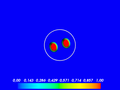
We display the results obtained for $\alpha=1$ , and $c_{m}=1.5,1.6$ in figure 2.

Here the box $\Omega$ in which all functions are supported (see subsection 5.1) has been chosen to be a square of diagonal length $\pi$ (and is represented by white lines). We emphasize that this box is needed to get the right minimizers, both theoretically and numerically. Theoretically, the condition that functions are supported in a fixed bounded set is needed for the compactness property (C) (again see subsection 5.1) to be satisfied, both in step one and in step two, as we let the size of the domain $T$ go to infinity. Numerically, without this box, for $c_{m}=1.5$ , simulations yield two balls (instead of one as shown on figure 1a) that get further and further away from each other as $T$ increases. But this configuration does not converge to an admissible candidate, so it definitely doesn’t converge to a minimizer.

We observe that for $c_{m}=1.6$ , we get two balls in opposite corners of the square $\Omega$ : it is consistent with the expected repulsive behaviour of the non-local term $\mathcal{V}_{\alpha}$ . Moreover, using (5.8) and (5.9), we find that, if conjecture 5.5 is true, there must be a minimizer up to $c_{m}\simeq 1.67$ . Numerically, we find that there is a minimizer up to a constant $c_{m}\in(1.5,1.6)$ , which is relatively close to $1.67$ . We also observe similar results for different values of $\alpha$ , including in the near field-dominated regime $\alpha<1$ .

For $\Omega$ a disk of diameter $\pi$ , if one increases further $c_{m}$ , we get three balls located near the boundary of $\Omega$ , as shown in figure 2a for $c_{m}=3.0$ . This is consistent with the conjecture that the energy is minimized by balls of the same volume. To illustrate the effect of the confining potential, we display in figure 2b the minimizer for $c_{m}=3.0$ , $A=1$ and $\beta=16$ .

Finally, let us mention that the number of discretization points is $N=2^{11}$ in each direction. Numerical minimization is made using the solver IPOPT [14]. The computation time on a standard computer is about an hour.

Appendix A Appendix: Study of the sets $\widetilde{S}_{}$ and $S_{}$ from the proof of proposition 3.3

In this appendix, we give explicit forms of the sets $\widetilde{S}_{*}$ and $S_{*}$ , needed in the proof of proposition 3.3. Let us define, for all $k\geq 2$ , a function $f_{k}:(0,\infty)\to\mathbb{R}$ by

f_{k}(\gamma)=1-\gamma^{1+\alpha}\frac{\mu_{k}^{\alpha}-\mu_{1}^{\alpha}}{\lambda_{k}-\lambda_{1}}+\gamma^{1+\beta}\frac{A\beta}{\lambda_{k}-\lambda_{1}}.

Then the sets $\widetilde{S}_{*}$ and $S_{*}$ from the proof of proposition 3.3 are defined by

\widetilde{S}_{*}=\{\forall k\geq 2,f_{k}>0\}\quad\text{and}\quad S_{*}=\{\forall k\geq 2,f_{k}\geq 0\}.

As stated in [6, equations (7.4), (7.5) and (7.6)], we have

\displaystyle\mu_{k}^{\alpha}=\begin{cases}\frac{2^{1+\alpha}\pi^{\frac{n-1}{2}}}{1-\alpha}\frac{\Gamma(\frac{1+\alpha}{2})}{\Gamma(\frac{n-\alpha}{2})}\left(\frac{\Gamma(k+\frac{n-\alpha}{2})}{\Gamma(k+\frac{n-2+\alpha}{2})}-\frac{\Gamma(\frac{n-\alpha}{2})}{\Gamma(\frac{n-2+\alpha}{2})}\right)&\text{if }\alpha\in(0,1),\\ 2^{\alpha}\pi^{\frac{n-1}{2}}\frac{\Gamma(\frac{\alpha-1}{2})}{\Gamma(\frac{n-\alpha}{2})}\left(\frac{\Gamma(\frac{n-\alpha}{2})}{\Gamma(\frac{n-2+\alpha}{2})}-\frac{\Gamma(k+\frac{n-\alpha}{2})}{\Gamma(k+\frac{n-2+\alpha}{2})}\right)&\text{if }\alpha\in(1,n),\\ \frac{4\pi^{\frac{n-1}{2}}}{\Gamma(\frac{n-1}{2})}\left(\frac{\Gamma^{\prime}(k+\frac{n-1}{2})}{\Gamma(k+\frac{n-1}{2})}-\frac{\Gamma^{\prime}(\frac{n-1}{2})}{\Gamma(\frac{n-1}{2})}\right)&\text{if }\alpha=1.\\ \end{cases}

(A.1)

Recall also that for any $k\geq 0$ , $\lambda_{k}=k(n+k-2)$ . Now let us treat each case enumerated in proposition 3.3 separately.

Case (i): $\alpha>\beta$ . A simple study of the sign of $f_{k}^{\prime}$ shows that each $f_{k}$ is increasing from $0$ to a point $\gamma_{k}$ , then decreasing from $\gamma_{k}$ to $+\infty$ . What is more $f_{k}(0)=1$ and $\lim_{+\infty}f_{k}=-\infty$ , so each $f_{k}$ has exactly one zero and is positive left of this zero and negative right of it. At last, for any constant $K>0$ , $f_{k}(\gamma)\displaystyle\mathop{\longrightarrow}_{k\rightarrow\infty}1$ uniformly in $\gamma\leq K$ . Putting these facts together shows that the sets $\widetilde{S}_{*}$ and $S_{*}$ have the forms:

\widetilde{S}_{*}=(0,m_{*})\quad\text{and}\quad S_{*}=(0,m_{*}],

for some critical mass $m_{*}>0$ (depending on $n$ , $\alpha$ , $\beta$ and $A$ ).

Case (ii): $\alpha=\beta$ . For any $k$ , $f_{k}$ is either decreasing or increasing or constant (depending on the size of $A$ ). If none of them is decreasing, then for any $k$ , $f_{k}\geq f_{k}(0)=1$ , so

\widetilde{S}_{*}=S_{*}=(0,+\infty).

Otherwise the same arguments as in case one shows again that

\widetilde{S}_{*}=(0,m_{*})\quad\text{and}\quad S_{*}=(0,m_{*}],

for some critical mass $m_{*}>0$ (depending on $n$ , $\alpha$ , $\beta$ and $A$ ).

Cases (iii), (iv) and (v): $\alpha<\beta$ . A simple study of the sign of $f_{k}^{\prime}$ shows that each $f_{k}$ is decreasing from $0$ to a point $\gamma_{k}$ , then increasing from $\gamma_{k}$ to $+\infty$ , and we have:

\gamma_{k}=\left(\frac{1+\alpha}{A\beta(1+\beta)}(\mu_{k}^{\alpha}-\mu_{1}^{\alpha})\right)^{\frac{1}{\beta-\alpha}}.

(A.2)

Another simple computation shows that

\min f_{k}=f_{k}(\gamma_{k})=1-\left(\frac{1+\alpha}{A\beta(1+\beta)}\right)^{\frac{1+\alpha}{\beta-\alpha}}\frac{\beta-\alpha}{1+\beta}\frac{(\mu_{k}^{\alpha}-\mu_{1}^{\alpha})^{\frac{1+\beta}{\beta-\alpha}}}{\lambda_{k}-\lambda_{1}}.

(A.3)

We must treat the subcases $\alpha>1$ , $\alpha=1$ and $\alpha<1$ separately.
Subcase one: $\alpha>1$ . We use the following classical Stirling formula:

\Gamma(x)\underset{x\to+\infty}{\sim}\sqrt{{\frac{2\pi}{x}}}\left(\frac{x}{e}\right)^{x},

to find that

\frac{\Gamma(k+\frac{n-\alpha}{2})}{\Gamma(k+\frac{n-2+\alpha}{2})}\underset{k\to\infty}{\sim}k^{1-\alpha}.

With (A.1), this means that the sequence $(\mu_{k}^{\alpha})$ is bounded. As $\lambda_{k}\displaystyle\mathop{\longrightarrow}_{k\rightarrow\infty}\infty$ , we get from (A.3)

\min f_{k}\displaystyle\mathop{\longrightarrow}_{k\rightarrow\infty}1.

Thus there exists an index $k_{0}$ such that

\widetilde{S}_{*}=\bigcap_{k=2}^{k_{0}}\{f_{k}>0\}\quad\text{and}\quad S_{*}=\bigcap_{k=2}^{k_{0}}\{f_{k}\geq 0\}.

(A.4)

As for any $k$ , $\lim_{+\infty}f_{k}=+\infty$ , we get that $\widetilde{S}_{*}$ and $S_{*}$ both contain an unbounded interval, which is what we wanted.
Subcase two: $\alpha=1$ . We use the classical asymptotics of the digamma function $\frac{\Gamma^{\prime}}{\Gamma}$ :

\frac{\Gamma^{\prime}}{\Gamma}(x)\underset{x\to+\infty}{\sim}\ln(x),

to find that, according to (A.3),

\min f_{k}\displaystyle\mathop{\longrightarrow}_{k\rightarrow+\infty}1.

We conclude as above.
Subcase three: $\alpha<1$ . Once again we use the asymptotics

\frac{\Gamma(k+\frac{n-\alpha}{2})}{\Gamma(k+\frac{n-2+\alpha}{2})}\underset{k\to\infty}{\sim}k^{1-\alpha},

to find that

\frac{(\mu_{k}^{\alpha}-\mu_{1}^{\alpha})^{\frac{1+\beta}{\beta-\alpha}}}{\lambda_{k}-\lambda_{1}}\underset{k\to\infty}{\sim}\frac{(k^{1-\alpha})^{\frac{1+\beta}{\beta-\alpha}}}{k^{2}}=k^{\frac{(1-\beta)(1+\alpha)}{\beta-\alpha}}.

(A.5)

If $\beta>1$ , once again we have

\min f_{k}\displaystyle\mathop{\longrightarrow}_{k\rightarrow+\infty}1,

and we conclude as above. If $\beta<1$ , then we have

\min f_{k}\displaystyle\mathop{\longrightarrow}_{k\rightarrow+\infty}-\infty

(A.6)

Also, by definition we have

f_{k+1}(\gamma_{k})-1=-\gamma_{k}^{1+\alpha}\frac{\mu_{k+1}^{\alpha}-\mu_{1}^{\alpha}}{\lambda_{k+1}-\lambda_{1}}+\gamma_{k}^{1+\beta}\frac{A\beta}{\lambda_{k+1}-\lambda_{1}}.

As the sequence $(\mu_{k}^{\alpha})$ is increasing we get

$\displaystyle f_{k+1}(\gamma_{k})-1$	$\displaystyle\leq-\gamma_{k}^{1+\alpha}\frac{\mu_{k}^{\alpha}-\mu_{1}^{\alpha}}{\lambda_{k+1}-\lambda_{1}}+\gamma_{k}^{1+\beta}\frac{A\beta}{\lambda_{k+1}-\lambda_{1}}$
	$\displaystyle=(f_{k}(\gamma_{k})-1)\frac{\lambda_{k}-\lambda_{1}}{\lambda_{k+1}-\lambda_{1}}$
	$\displaystyle\displaystyle\mathop{\longrightarrow}_{k\rightarrow\infty}-\infty.$	(A.7)

With (A.6), this means that

[\gamma_{k},\gamma_{k+1}]\subset(\widetilde{S}_{*})^{\mathsf{c}}\cap(S_{*})^{\mathsf{c}}.

What is more, from (A.2), we have $\gamma_{k}\displaystyle\mathop{\longrightarrow}_{k\rightarrow+\infty}+\infty$ , so $\widetilde{S}_{*}$ and $S_{*}$ are both bounded, which is what we wanted. At last, if $\beta=1$ we find using (A.5) that there exists a constant $C_{\alpha}$ such that

\min f_{k}\displaystyle\mathop{\longrightarrow}_{k\rightarrow\infty}1-\frac{C_{\alpha}}{A^{\frac{1+\alpha}{\beta-\alpha}}}.

For $A^{\frac{1+\alpha}{\beta-\alpha}}>C_{\alpha}$ , we conclude as in case one. For $A^{\frac{1+\alpha}{\beta-\alpha}}<C_{\alpha}$ , we conclude as above that $\widetilde{S}_{*}$ and $S_{*}$ are both bounded. For $A^{\frac{1+\alpha}{\beta-\alpha}}<C_{\alpha}$ , we have to use the following more precise form of Stirling’s approximation:

\Gamma(x)\underset{x\to+\infty}{\sim}\sqrt{{\frac{2\pi}{x}}}\left(\frac{x}{e}\right)^{x}(1+O(\frac{1}{x})).

Proceeding to simple asymptotic expansions, we find that for $k$ large enough we have

\min f_{k}>0.

We conclude as in case one.

Appendix B Computation of $\mathcal{V}_{\alpha}(B[1])$

Here we explain how we compute $\mathcal{V}_{\alpha}(B[1])$ numerically, as needed in subsection 5.2 to choose the value of $T$ . In order to compute numerically the improper integral

\mathcal{V}_{\alpha}(B[1])=\int_{B[1]\times B[1]}\frac{\mathrm{d}x\mathrm{d}y}{\left|x-y\right|^{2-\alpha}},

we add a small term $\epsilon>0$ to the denominator of the integrand. So we compute

\mathcal{V}_{\alpha,\epsilon}(B[1])=\int_{B[1]\times B[1]}\frac{\mathrm{d}x\mathrm{d}y}{\left|x-y\right|^{2-\alpha}+\epsilon}.

To control the error introduced by the parameter $\epsilon$ , we need to estimate the difference $\Delta_{\epsilon}:=\mathcal{V}_{\alpha}(B[1])-\mathcal{V}_{\alpha,\epsilon}(B[1])$ . We have

	$\displaystyle\Delta_{\epsilon}$	$\displaystyle=\int_{B[1]\times B[1]}\frac{\mathrm{d}x\mathrm{d}y}{\left\|x-y\right\|^{2-\alpha}}-\int_{B[1]\times B[1]}\frac{\mathrm{d}x\mathrm{d}y}{\left\|x-y\right\|^{2-\alpha}+\epsilon}$
		$\displaystyle=\int_{B[1]\times B[1]}\frac{\epsilon\mathrm{d}x\mathrm{d}y}{\left\|x-y\right\|^{2-\alpha}(\left\|x-y\right\|^{2-\alpha}+\epsilon)}$
		$\displaystyle\leq\int_{B[1]\times B[1]}\mathds{1}_{\left\|x-y\right\|<r}\frac{\mathrm{d}x\mathrm{d}y}{\left\|x-y\right\|^{2-\alpha}}+\int_{B[1]\times B[1]}\mathds{1}_{\left\|x-y\right\|\geq r}\frac{\epsilon\mathrm{d}x\mathrm{d}y}{\left\|x-y\right\|^{2-\alpha}r^{2-\alpha}}$
		$\displaystyle\leq\int_{B[1]\times\mathbb{R}^{2}}\mathds{1}_{\left\|x-y\right\|<r}\frac{\mathrm{d}x\mathrm{d}y}{\left\|x-y\right\|^{2-\alpha}}+\frac{\epsilon}{r^{2-\alpha}}\int_{B[1]\times B[1]}\frac{\mathrm{d}x\mathrm{d}y}{\left\|x-y\right\|^{2-\alpha}}$
		$\displaystyle\leq\int_{B[1]\times\mathbb{R}^{2}}\mathds{1}_{\left\|y\right\|<r}\frac{\mathrm{d}x\mathrm{d}y}{\left\|y\right\|^{2-\alpha}}+\frac{\epsilon}{r^{2-\alpha}}\int_{B[1]}\int_{B[1]}\frac{\mathrm{d}x\mathrm{d}y}{\left\|y\right\|^{2-\alpha}}$
		$\displaystyle=\int_{\left\|y\right\|<r}\frac{\mathrm{d}y}{\left\|y\right\|^{2-\alpha}}+\frac{\epsilon}{r^{2-\alpha}}\int_{B[1]}\frac{\mathrm{d}y}{\left\|y\right\|^{2-\alpha}}$
		$\displaystyle=2\pi\int_{0}^{r}\frac{r^{2-1}\mathrm{d}r}{r^{2-\alpha}}+\frac{\epsilon}{r^{2-\alpha}}2\pi\int_{0}^{\frac{1}{\sqrt{\pi}}}\frac{r^{2-1}\mathrm{d}r}{r^{2-\alpha}}$
		$\displaystyle=\frac{2\pi}{\alpha}(r^{\alpha}+\frac{\epsilon}{r^{2-\alpha}\pi^{\frac{\alpha}{2}}}),$

for some $r>0$ . This last bound attains its minimum for $r=\left(\frac{(2-\alpha)\epsilon}{\alpha\pi^{\frac{\alpha}{2}}}\right)^{\frac{1}{2}}$ . From there we deduce

\Delta_{\epsilon}\leq\frac{2\pi}{\alpha}\frac{2}{2-\alpha}\left(\frac{2-\alpha}{\alpha}\right)^{\frac{\alpha}{2}}\left(\frac{\epsilon}{\pi^{\frac{\alpha}{2}}}\right)^{\frac{\alpha}{2}}.

With $\alpha=1$ , we get

\Delta_{\epsilon}\leq 4\pi^{\frac{3}{4}}\sqrt{\epsilon}.

Now the proper integral $\mathcal{V}_{\alpha,\epsilon}(B[1])$ can be expressed in polar coordinates, and computed with arbitrary precision in the Julia language, using the HCubature package.

References

[1] Stan Alama, Lia Bronsard, Rustum Choksi, and Ihsan Topaloglu. Droplet breakup in the liquid drop model with background potential. arXiv preprint arXiv:1708.04292, 2017.
[2] Stan Alama, Lia Bronsard, Rustum Choksi, and Ihsan Topaloglu. Ground-states for the liquid drop and tfdw models with long-range attraction. Journal of Mathematical Physics, 58(10):103503, 2017.
[3] Marco Bonacini and Riccardo Cristoferi. Local and global minimality results for a nonlocal isoperimetric problem on $\mathbb{R}^{N}$ . SIAM Journal on Mathematical Analysis, 46(4):2310–2349, 2014.
[4] Andrea Braides. Gamma-convergence for Beginners, volume 22. Clarendon Press, 2002.
[5] Rustum Choksi and Mark A Peletier. Small volume-fraction limit of the diblock copolymer problem: Ii. diffuse-interface functional. SIAM Journal on Mathematical Analysis, 43(2):739–763, 2011.
[6] Alessio Figalli, Nicola Fusco, Francesco Maggi, Vincent Millot, and Massimiliano Morini. Isoperimetry and stability properties of balls with respect to nonlocal energies. Communications in Mathematical Physics, 336(1):441–507, 2015.
[7] Rupert L Frank, Rowan Killip, and Phan Thành Nam. Nonexistence of large nuclei in the liquid drop model. Letters in Mathematical Physics, 106(8):1033–1036, 2016.
[8] Enrico Giusti. Minimal surfaces and functions of bounded variation, volume 80. Birkhauser Verlag, 1984.
[9] Hans Knüpfer and Cyrill B Muratov. On an isoperimetric problem with a competing nonlocal term i: The planar case. Communications on Pure and Applied Mathematics, 66(7):1129–1162, 2013.
[10] Elliott H Lieb and Michael Loss. Analysis, volume 14 of graduate studies in mathematics. American Mathematical Society, Providence, RI,, 4, 2001.
[11] Jianfeng Lu and Felix Otto. Nonexistence of a minimizer for thomas–fermi–dirac–von weizsäcker model. Communications on pure and applied mathematics, 67(10):1605–1617, 2014.
[12] Cyrill Muratov and Hans Knüpfer. On an isoperimetric problem with a competing nonlocal term ii: The general case. Communications on Pure and Applied Mathematics, 67(12):1974–1994, 2014.
[13] Elias M Stein. Singular integrals and differentiability properties of functions (PMS-30), volume 30. Princeton university press, 2016.
[14] A. Wächter and L. T. Biegler. On the implementation of a primal-dual interior point filter line search algorithm for large-scale nonlinear programming. Mathematical Programming, 106(1):25–27, 2006.

François Générau: Laboratoire Jean Kuntzmann (LJK), Université Joseph Fourier
Bâtiment IMAG, 700 avenue centrale, 38041 Grenoble Cedex 9 - FRANCE
francois.generau@univ-grenoble-alpes.fr

Edouard Oudet: Laboratoire Jean Kuntzmann (LJK), Université Joseph Fourier
Bâtiment IMAG, 700 avenue centrale, 38041 Grenoble Cedex 9 - FRANCE
edouard.oudet@univ-grenoble-alpes.fr
http://www-ljk.imag.fr/membres/Edouard.Oudet/

	$\displaystyle\mathcal{U}_{\beta,A}(E)-\mathcal{U}_{\beta,A}(B)$	$\displaystyle=\int_{E\setminus B}A\left\|x\right\|^{\beta}\mathrm{d}x-\int_{B\setminus E}A\left\|x\right\|^{\beta}\mathrm{d}x$
		$\displaystyle\geq\int_{\{x\in\mathbb{R}^{n}\colon 1\leq\left\|x\right\|\leq r_{2}\}}A\left\|x\right\|^{\beta}\mathrm{d}x-\int_{\{x\in\mathbb{R}^{n}\colon r_{1}\leq\left\|x\right\|\leq 1\}}A\left\|x\right\|^{\beta}\mathrm{d}x$
(for $x\to\left\|x\right\|^{\beta}$ is symmetric non-decreasing),
		$\displaystyle=AP(B)\left(\int_{1}^{r_{2}}r^{\beta}r^{n-1}\mathrm{d}r-\int_{r_{1}}^{1}r^{\beta}r^{n-1}\mathrm{d}r\right)$
		$\displaystyle=\frac{AP(B)}{n+\beta}\left(r_{2}^{n+\beta}-1-\left(1-r_{1}^{n+\beta}\right)\right)$
		$\displaystyle=\frac{AP(B)}{n+\beta}\left(\left(1+n\frac{\left\|E\setminus B\right\|}{P(B)}\right)^{\frac{n+\beta}{n}}-1\right.$
		$\displaystyle\qquad\left.{}-\left(1-\left(1-n\frac{\left\|E\setminus B\right\|}{P(B)}\right)^{\frac{n+\beta}{n}}\right)\right).$	(4.3)

	$\displaystyle[u]^{2}_{\frac{1-\alpha}{2}}$	$\displaystyle\leq\int_{\partial B\times\partial B}\frac{2(\left\|u(x)\right\|^{2}+\left\|u(y)\right\|)^{2}}{\left\|x-y\right\|^{n-\alpha}}\mathrm{d}\mathcal{H}^{n-1}(x)\mathrm{d}\mathcal{H}^{n-1}(y)$
		$\displaystyle=4\int_{\partial B\times\partial B}\frac{\left\|u(x)\right\|^{2}}{\left\|x-y\right\|^{n-\alpha}}\mathrm{d}\mathcal{H}^{n-1}(x)\mathrm{d}\mathcal{H}^{n-1}(y)$
		$\displaystyle=4\int_{\partial B}\left(\int_{\partial B}\frac{\mathrm{d}\mathcal{H}^{n-1}(y)}{\left\|x-y\right\|^{n-\alpha}}\right)\left\|u(x)\right\|^{2}\mathrm{d}\mathcal{H}^{n-1}(x)$
		$\displaystyle=C(n,\alpha)\int_{\partial B}\left\|u(x)\right\|^{2}\mathrm{d}\mathcal{H}^{n-1}(x)$
		$\displaystyle=C(n,\alpha)\\|u\\|_{L^{2}(\partial B)}^{2},$

	$\displaystyle\Delta_{\epsilon}$	$\displaystyle=\int_{B[1]\times B[1]}\frac{\mathrm{d}x\mathrm{d}y}{\left\|x-y\right\|^{2-\alpha}}-\int_{B[1]\times B[1]}\frac{\mathrm{d}x\mathrm{d}y}{\left\|x-y\right\|^{2-\alpha}+\epsilon}$
		$\displaystyle=\int_{B[1]\times B[1]}\frac{\epsilon\mathrm{d}x\mathrm{d}y}{\left\|x-y\right\|^{2-\alpha}(\left\|x-y\right\|^{2-\alpha}+\epsilon)}$
		$\displaystyle\leq\int_{B[1]\times B[1]}\mathds{1}_{\left\|x-y\right\|<r}\frac{\mathrm{d}x\mathrm{d}y}{\left\|x-y\right\|^{2-\alpha}}+\int_{B[1]\times B[1]}\mathds{1}_{\left\|x-y\right\|\geq r}\frac{\epsilon\mathrm{d}x\mathrm{d}y}{\left\|x-y\right\|^{2-\alpha}r^{2-\alpha}}$
		$\displaystyle\leq\int_{B[1]\times\mathbb{R}^{2}}\mathds{1}_{\left\|x-y\right\|<r}\frac{\mathrm{d}x\mathrm{d}y}{\left\|x-y\right\|^{2-\alpha}}+\frac{\epsilon}{r^{2-\alpha}}\int_{B[1]\times B[1]}\frac{\mathrm{d}x\mathrm{d}y}{\left\|x-y\right\|^{2-\alpha}}$
		$\displaystyle\leq\int_{B[1]\times\mathbb{R}^{2}}\mathds{1}_{\left\|y\right\|<r}\frac{\mathrm{d}x\mathrm{d}y}{\left\|y\right\|^{2-\alpha}}+\frac{\epsilon}{r^{2-\alpha}}\int_{B[1]}\int_{B[1]}\frac{\mathrm{d}x\mathrm{d}y}{\left\|y\right\|^{2-\alpha}}$
		$\displaystyle=\int_{\left\|y\right\|<r}\frac{\mathrm{d}y}{\left\|y\right\|^{2-\alpha}}+\frac{\epsilon}{r^{2-\alpha}}\int_{B[1]}\frac{\mathrm{d}y}{\left\|y\right\|^{2-\alpha}}$
		$\displaystyle=2\pi\int_{0}^{r}\frac{r^{2-1}\mathrm{d}r}{r^{2-\alpha}}+\frac{\epsilon}{r^{2-\alpha}}2\pi\int_{0}^{\frac{1}{\sqrt{\pi}}}\frac{r^{2-1}\mathrm{d}r}{r^{2-\alpha}}$
		$\displaystyle=\frac{2\pi}{\alpha}(r^{\alpha}+\frac{\epsilon}{r^{2-\alpha}\pi^{\frac{\alpha}{2}}}),$

Large volume minimizers of a non-local isoperimetric problem: theoretical and numerical approaches

Abstract

1 Introduction

Theorem 1.1.

Theorem 1.2.

2 Existence of a minimizer in (1.2)

Proposition 2.1.

Notation.

Proof.

Remark 2.2.

3 Extension of some known results

Proposition 3.1.

Terminology 3.2.

Proposition 3.3.

Remark 3.4.

Ideas of the proof.

4 Large volume minimizers for α<β\alpha<\beta

4.1 Hausdorff convergence of large volume minimizers for α<β{\alpha<\beta}

Lemma 4.1.

Lemma 4.2.

Proof.

Proof of lemma 4.1.

Proof of theorem 1.1.

Remark 4.3.

Lemma 4.4.

Proof.

4.2 Large volume minimizers = balls for α<β\alpha<\beta and β>1\beta>1

Lemma 4.5.

Proof of theorem 1.2.

Lemma 4.6.

Lemma 4.7.

Proof of lemma 4.7.

5 Numerical minimization

5.1 Method of the numerical minimization

Terminology 5.1.

Remark 5.2.

Lemma 5.3.

Proof of (5.7).

5.2 Numerical results

Conjecture 5.4.

Conjecture 5.5.

Appendix A Appendix: Study of the sets S~∗\widetilde{S}_{*} and S∗S_{*} from the proof of proposition 3.3

Appendix B Computation of 𝒱α​(B​[1])\mathcal{V}_{\alpha}(B[1])

References

4 Large volume minimizers for $\alpha<\beta$

4.1 Hausdorff convergence of large volume minimizers for ${\alpha<\beta}$

4.2 Large volume minimizers = balls for $\alpha<\beta$ and $\beta>1$

Appendix A Appendix: Study of the sets $\widetilde{S}_{}$ and $S_{}$ from the proof of proposition 3.3

Appendix B Computation of $\mathcal{V}_{\alpha}(B[1])$