Single-atom transistor as a precise magnetic field sensor
Abstract
Feshbach resonances, which allow for tuning the interactions of ultracold atoms with an external magnetic field, have been widely used to control the properties of quantum gases. We propose a scheme for using scattering resonances as a probe for external fields, showing that by carefully tuning the parameters it is possible to reach a G (or nT) level of precision with a single pair of atoms. We show that for our collisional setup it is possible to saturate the quantum precision bound with a simple measurement protocol.
Introduction. Quantum technologies hold the promise for significant advancement in various fields such as communication and sensing due to the potential to utilize quantum coherence or entanglement to improve the performance of devices. In recent years, great progress has been made in bringing quantum-enhanced sensing towards practical and industrial applications [1, 2]. Here the goal is to construct specific quantum systems for the precise measurement of external parameters such as electromagnetic fields. This is crucial in a range of domains from fundamental [3, 4, 5, 6, 7, 8, 9] to technological applications e.g. in medicine or materials science, where detection of fields produced by single spins is often desired [10].
The state-of-the-art magnetic field sensing techniques exploit field-dependent effects in a number of different systems. Outstanding sensitivity to ac signals is obtained by the superconducting quantum interference devices (SQUID) [11, 12]. Other systems that reach high performance are based on nitrogen-vacancy centres in diamonds [13, 14, 15], thermal atomic vapors [16, 17], internal states of trapped ions [18, 19], and the cold or ultracold atomic samples [20, 21, 22, 23, 24, 25, 26, 27]. Ultracold atoms are a natural candidate for implementing quantum sensing protocols, since they offer the possibility of working with large ensembles of particles prepared in a very well defined initial quantum state. Due to low (sub-K) temperatures, cold atoms can be trapped using external electromagnetic fields such as optical lattices [28]. Interestingly, interatomic interactions can also be tuned in an experiment if a Feshbach resonance is available [29, 30]. The resonance mechanism originates from the coupling of the free atomic pair to a bound state. Typically the different scattering channels are associated with the hyperfine structure of the atoms, which allows to tune the position of the bound state via magnetic field by means of the differential Zeeman shift.
The interplay of controlled interactions and external confinement has been the subject of intense studies, both experimental [31, 32, 33] and theoretical [34, 35, 36, 37, 38, 39, 40, 41, 42, 43, 44, 45, 46, 47]. Confinement-induced resonances, which result from the modification of scattering properties by the external trap, allowed for controlling atomic interactions of ultracold bosons in low dimensions, leading to the experimental realization of the long-sought Tonks-Girardeau gas [48, 49].
In this Letter, we propose to look at the resonances from a different angle. Instead of tuning the collisional properties of atoms with external fields, we treat the collisions as a probe of the field itself. We consider a simple scheme in which the atoms are colliding in quasi-one-dimensional (1D) waveguides created e.g. by an optical lattice. In the vicinity of a Feshbach resonance, the collisional phase shift strongly depends on the external magnetic field. Information about the field strength can be extracted e.g. by measuring the transmission of atoms through the waveguides. The performance of this measurement can be assessed by means of the Quantum Cramér-Rao lower bound (QCRLB), which provides the ultimate limit on the uncertainty of the inferred magnetic field [50].
Sensor construction. The sensor we have in mind is schematically illustrated in Fig. 1. An ensemble of noninteracting atoms is injected into a set of quasi-one-dimensional waveguides realized by using a deep 3D optical lattice relaxed in the longitudinal direction. In the center of every waveguide there is a tightly confined impurity atom, either from a different hyperfine state or different species, tightly trapped by an optical potential using a magic wavelength transparent for the incoming atoms [51]. The sensitivity to magnetic fields is provided by the Feshbach resonance, which controls the interaction between the atom and the impurity characterized by the 3D scattering length . The transverse width of the waveguides is chosen in such a way that the probability of reflecting the colliding atom back from the impurity strongly depends on the value of the magnetic field, which is explained in detail further. The efficient detection of the transmitted single atoms at the end of the waveguides can be accomplished in several ways, for example by ionization or absorption imaging. From the counting statistics it is then possible to infer the strength of the magnetic field with the precision attaining the classical Cramér-Rao bound. As shown in Fig. 1, the spatial separation of the tubes typically of the order of 500 nm naturally provides high spatial resolution. Systems with desired properties can be realized with state-of-the-art techniques used in ultracold atomic quantum gas experiments (see e.g. [52, 53]).
Atomic scattering in quasi-one-dimensional geometry. Let us now briefly review the relevant two-body physics taking place in a single tube. We assume the impurity atoms are pinned by the trap [54]. The stationary Schrödinger equation for the incoming atom then reads
| (1) |
Here is the transverse trap which we assume to be harmonic (), and is the trap frequency. The parameters can be combined into a characteristic lengthscale . Finally, is the interparticle interaction with characteristic range much smaller than and it can be described by the pseudopotential [28, 54]
| (2) |
Here is the reduced mass of the pair of atoms, and the energy-dependent scattering length is defined as , where denotes the phase shift in the partial wave . The scattering length depends on the magnetic field due to a Feshbach resonance and in the zero energy limit can be described by the simple relation [30]
| (3) |
where is the background scattering length away from the resonance, denotes the resonance width, and is the resonance position. In order to work in the incoming atoms reference frame we rewrite eq. (2) as with . Here is the total energy of the relative motion , where is the one-dimensional wavenumber.
In the presence of a strong transverse confinement one can assume that the asymptotic wave function is well described by the lowest mode of the transverse harmonic oscillator. The transmission coefficient, which describes the part of the flux that goes through the tube, can then be defined as [34], with being the one-dimensional phase shift given by [38]
| (4) |
Here and is the Hurwitz zeta function.
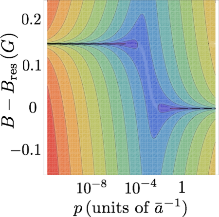
In Fig. 2 we show the dependence of the transmission coefficient on the magnetic field computed for two exemplary Feshbach resonances generated numerically using a two-channel model with van der Waals interactions in a quasi-1D harmonic trap. For the length unit we use defined as the mean characteristic length of the van der Waals potential [55], which is typically of the order of . Optical lattice confinement leads to values of of around [32] while we choose . At the position of the so-called confinement-induced resonance (CIR) given by , diverges and the transmission reaches zero. One can also observe the opposite case of unit transmission, where the atoms are effectively noninteracting near the zero crossing of the 3D scattering length. Both features can in principle be used for magnetic field measurement. We note that while the CIR feature becomes sharper as the collision energy increases, the unit transmission peak becomes less pronounced. This is because the background transmission grows with energy.
Sensor performance. We proceed with the analysis of the achievable sensor performance. The classical Cramér-Rao lower bound (CRLB) is a general theorem from estimation theory that provides a lower bound on the uncertainty of the inferred value of an unknown parameter [50, 56, 57]. In our case, this bound can be expressed in the form of the inequality for the estimation uncertainty : , where is the classical Fisher information [56] which quantifies the usefulness of the metrological protocol and is the number of atoms. The Fisher information is expressed in terms of the probability distribution of different outcomes
| (5) |
where the transmission probability is , and the probability of reflecting the atom is . The CRLB is saturated asymptotically by the maximum likelihood estimator in the limit of a large number of atoms used in the estimation procedure.
Expressing the probability distributions in terms of the transmission coefficient , the Fisher information takes the form
| (6) |
The structure of this formula is intuitively clear, as the most favourable conditions are attained when the transmission strongly depends on the magnetic field. The uncertainty is further reduced by the statistical enhancement factor , where denotes the number of repetitions (or atoms per tube). Hence, with a limited experimental effort, one can easily improve the sensor sensitivity by several orders of magnitude.
Choice of resonance parameters. Figure 3 displays the precision by means of Eq. (6) for the same parameters as in Fig. 2. Quite strikingly, depending on the background scattering length, the precision has a different dependence on the collision energy and it can take the highest values either at the CIR or at the unit transmission peak. This can be explained by extracting the leading order behavior of Eq. (6). Neglecting finite energy corrections, we obtain that
| (7) |
at the CIR and
| (8) |
at the unit transmission peak. In both cases scales linearly with the resonance width , which gives a natural scale for the detection uncertainty. However, at the CIR a low background scattering length and a certain finite is preferred, while at the unit transmission peak a high and a very low energy gives better results. These simple bounds are in good agreement with the general formula (6) and are summarized in Fig. 4.


Let us now discuss the realistic conditions for the implementation of the sensor. For measuring at the unit transmission peak, it is preferred to work with high background scattering length which is typically expected e.g. in ion-atom mixtures or between Cs atoms. However, in order to achieve the highest precision for this case, it is required to reduce the collision energy to sub-nK regime. To be able to work at more reasonable temperatures it is better to switch to the CIR and low . Here the most promising systems are the ones involving lanthanide atoms such as dysprosium and erbium, which can feature tens of narrow resonances per Gauss along with a few broad resonances that set the local background [58, 59, 60]. This ensures that one can find at least a few resonances with the desired properties. Scattering of lanthanide atoms includes sizeable dipolar contribution [54] and represents a challenge for a full theoretical description and is the subject of intense investigations [61, 62]. Finding a resonance with G in the region where leads to a precision of the order of G (single nanotesla) with a single atom at reasonable energies nK.
Discussion. We proceed with discussing the main potential error sources. The first limiting factor is the finite width of the longitudinal momentum distribution. In the case of measuring at unit transmission, this can impose stringent limits as one has to reduce the energy as much as possible. However, as can be seen from the right panel of Fig. 4, for measuring at the CIR has a rather broad minimum. In addition, one has to consider fluctuations of the resonance position due to finite energy corrections given by the differential magnetic moment , which typically is of the order of several MHz per Gauss [30]. This results in uncertainty of the order of G for energy distribution width of 1 nK. This estimation shows that the momentum has to be quite precisely controlled.
Furthermore, the details of the trapping potentials and interatomic interactions can lead to emergence of additional narrow resonances along with a shift of the -wave CIR position. These system-specific effects have to be included, but do not affect the precision bounds [54].
In addition, the uncertainty of the estimated magnetic field strength depends on the efficiency of the detector, denoted by . Let us assume first that we measure whether the atom injected into the tube was transmitted or reflected. Then, the probability of detecting the transmitted (reflected) atom is given by . In such a case, the Fisher information is simply given by , where is the Fisher information for the perfect detectors given by Eq. (5) and the attainable uncertainty is rescaled by a factor .
In another scenario one can measure only the transmitted atoms and the reflected atoms are not monitored. In this case, the fact that we do not detect an atom can be due either to reflection or to the detector inefficiency. Therefore, the probability of registering the transmitted atom is , whereas the probability of not detecting this atom is . Consequently, the Fisher information is given by . In the limit we recover the result for two perfect detectors.
In the proposed scheme we measure only the number of atoms that were transmitted through the impurity. It is natural to ask about the maximal attainable precision utilizing a different measurement. To answer this question we refer to the QCRLB, which provides the lower bound for the precision of any measurement allowed by quantum mechanics. In [54], we show that the measurement we propose yields a precision of the magnetic field that saturates this bound. As a consequence, a different measurement strategy, preceded optionally by any operation on the state of the system after the collision, will not improve the precision further. This result can be understood as follows. After the collision the particle is in a superposition of being transmitted or reflected with respective probability amplitudes. The modulus and phase of these amplitudes depend on the magnetic field. The measurement we propose is only capable of determining the moduli of the amplitudes, but the information about the field encoded in the phases is lost. However, the phases of the amplitudes are equal and form a common phase factor. As a consequence, in our situation, the full information about the magnetic field is contained in the moduli of the amplitudes, and, thus, the measurement is optimal [63].
Finally, let us compare the performance of our collisional sensor to other available magnetic field sensing methods. At this point it is convenient to take into account that accumulation of the data improves the sensitivity. The scaling with the number of repetitions improves the precision by a factor . Denoting the time for detecting a single collision event by , during the total time of the experiment repetitions are made. For reasonable times of the order of a few tens of miliseconds, the achievable precision scales with as . The sensor we propose is sensitive to static (dc) magnetic fields, and thus works in a different regime than SQUIDs, trapped ions or NV centers. Its small radial size of the order of a few tens of nanometers makes it especially useful for probing the local magnetic field directly in the experiments based on cold atoms. Furthermore, with the optical lattice forming the waveguides, the sensor can work as a parallel, multipoint scanning probe capable of measuring local magnetic fields with a sub-micron resolution limited by the lattice spacing. This configuration can be valuable for measuring the field gradients. The combination of high resolution with nanotesla precision is unique compared to other methods of dc field sensing (see Fig. 4 in [25] for a detailed comparison).
Conclusions. We have demonstrated that Feshbach and confinement-induced resonances can make cold collisions useful from a quantum sensing point of view. We identified an optimal measurement scheme in which both reflected and transmitted atoms are monitored after the scattering event. We proved that in this approach the sensitivity of the magnetic field is maximal and we saturate the Quantum Cramér-Rao lower bound. This approach can allow for ultraprecise characterization of Feshbach resonances, overcoming the three-body loss measurements which are sensitive to temperature effects and detailed structure of the three-body bound states. It might find application in precise determination of the residual magnetic fields for improved precision of optical lattice clocks. It would also be interesting to extend the scheme beyond magnetic field measurements. It is well known that Feshbach resonances can be controlled with external laser and rf fields, making cold collisions a possibly versatile sensor.
This work was supported by the Alexander von Humboldt Foundation, the Polish National Science Center project 2014/14/M/ST2/00015, the cluster of excellence The Hamburg Centre for Ultrafast Imaging of the Deutsche Forschungsgemeinschaft, and the European Union FP7 FET Proactive project DIADEMS (grant N. 611143).
References
- [1] V. Giovannetti, S. Lloyd, and L. Maccone, Phys. Rev. Lett. 96, 010401 (2006).
- [2] C. L. Degen, F. Reinhard, and P. Cappellaro, Rev. Mod. Phys. 89, 035002 (2017).
- [3] J. K. Webb, V. V. Flambaum, C. W. Churchill, M. J. Drinkwater, and J. D. Barrow, Phys. Rev. Lett. 82, 884 (1999).
- [4] C. Chin and V. V. Flambaum, Phys. Rev. Lett. 96, 230801 (2006).
- [5] T. Zelevinsky, S. Kotochigova, and J. Ye, Phys. Rev. Lett. 100, 043201 (2008).
- [6] S. Blatt, A. Ludlow, G. Campbell, J. W. Thomsen, T. Zelevinsky, M. Boyd, J. Ye, X. Baillard, M. Fouché, R. Le Targat, et al., Phys. Rev. Lett. 100, 140801 (2008).
- [7] R. Schnabel, N. Mavalvala, D. E. McClelland, and P. K. Lam, Nat. Comm. 1, 121 (2010).
- [8] J. J. Hudson, D. M. Kara, I. Smallman, B. E. Sauer, M. R. Tarbutt, and E. A. Hinds, Nature 473, 493 (2011).
- [9] J. Baron, W. C. Campbell, D. DeMille, J. M. Doyle, G. Gabrielse, Y. V. Gurevich, P. W. Hess, N. R. Hutzler, E. Kirilov, I. Kozyryev, et al., Science 343, 269 (2014).
- [10] G. Balasubramanian, I. Chan, R. Kolesov, M. Al-Hmoud, J. Tisler, C. Shin, C. Kim, A. Wojcik, P. R. Hemmer, A. Krueger, et al., Nature 455, 648 (2008).
- [11] R. C. Jaklevic, J. Lambe, A. H. Silver, and J. E. Mercereau, Phys. Rev. Lett. 12, 159 (1964).
- [12] D. Vasyukov, Y. Anahory, L. Embon, D. Halbertal, J. Cuppens, L. Neeman, A. Finkler, Y. Segev, Y. Myasoedov, M. L. Rappaport, et al., Nature Nanotechnology 8, 639 (2013).
- [13] J. Maze, P. Stanwix, J. Hodges, S. Hong, J. Taylor, P. Cappellaro, L. Jiang, M. G. Dutt, E. Togan, A. Zibrov, et al., Nature 455, 644 (2008).
- [14] T. Wolf, P. Neumann, K. Nakamura, H. Sumiya, T. Ohshima, J. Isoya, and J. Wrachtrup, Phys. Rev. X 5, 041001 (2015).
- [15] S. Zaiser, T. Rendler, I. Jakobi, T. Wolf, S.-Y. Lee, S. Wagner, V. Bergholm, T. Schulte-Herbrüggen, P. Neumann, and J. Wrachtrup, Nat. Comm. 7 (2016).
- [16] V. G. Lucivero, P. Anielski, W. Gawlik, and M. W. Mitchell, Rev. Sci. Instrum. 85, 113108 (2014).
- [17] W. Wasilewski, K. Jensen, H. Krauter, J. J. Renema, M. V. Balabas, and E. S. Polzik, Phys. Rev. Lett. 104, 133601 (2010).
- [18] I. Baumgart, J. Can, A. Retzker, M. Plenio, and C. Wunderlich, Phys. Rev. Lett. 116, 240801 (2016).
- [19] S. Kotler, N. Akerman, Y. Glickman, A. Keselman, and R. Ozeri, Nature 473, 61â65 (2011).
- [20] I. K. Kominis, T. W. Kornack, J. C. Allred, and M. V. Romalis, Nature 422, 596 (2003).
- [21] S. Wildermuth, S. Hofferberth, I. Lesanovsky, E. Haller, L. M. Andersson, S. Groth, I. Bar-Joseph, P. Krüger, and J. Schmiedmayer, Nature 435, 440 (2005).
- [22] M. Vengalattore, J. M. Higbie, S. R. Leslie, J. Guzman, L. E. Sadler, and D. M. Stamper-Kurn, Phys. Rev. Lett. 98, 200801 (2007).
- [23] M. Koschorreck, M. Napolitano, B. Dubost, and M. Mitchell, Appl. Phys. Lett. 98, 074101 (2011).
- [24] N. Behbood, F. Martin Ciurana, G. Colangelo, M. Napolitano, M. W. Mitchell, and R. J. Sewell, Appli. Phys. Lett. 102, 173504 (2013).
- [25] F. Yang, A. J. Kollár, S. F. Taylor, R. W. Turner, and B. L. Lev, Phys. Rev. Applied 7, 034026 (2017).
- [26] F. Martin Ciurana, G. Colangelo, L. Slodička, R. J. Sewell, and M. W. Mitchell, Phys. Rev. Lett. 119, 043603 (2017).
- [27] Q.-Q. Hu, C. Freier, B. Leykauf, V. Schkolnik, J. Yang, M. Krutzik, and A. Peters, Phys. Rev. A 96, 033414 (2017).
- [28] I. Bloch, J. Dalibard, and W. Zwerger, Rev. Mod. Phys. 80, 885 (2008).
- [29] J. Weiner, V. S. Bagnato, S. Zilio, and P. S. Julienne, Rev. Mod. Phys. 71, 1 (1999).
- [30] C. Chin, R. Grimm, P. Julienne, and E. Tiesinga, Rev. Mod. Phys. 82, 1225 (2010).
- [31] H. Moritz, T. Stöferle, K. Günter, M. Köhl, and T. Esslinger, Phys. Rev. Lett. 94, 210401 (2005).
- [32] E. Haller, M. J. Mark, R. Hart, J. G. Danzl, L. Reichsöllner, V. Melezhik, P. Schmelcher, and H.-C. Nägerl, Phys. Rev. Lett. 104, 153203 (2010).
- [33] S. Sala, G. Zürn, T. Lompe, A. N. Wenz, S. Murmann, F. Serwane, S. Jochim, and A. Saenz, Phys. Rev. Lett. 110, 203202 (2013).
- [34] M. Olshanii, Phys. Rev. Lett. 81, 938 (1998).
- [35] E. Tiesinga, C. J. Williams, F. H. Mies, and P. S. Julienne, Phys. Rev. A 61, 063416 (2000).
- [36] D. Petrov and G. Shlyapnikov, Physical Review A 64, 012706 (2001).
- [37] E. L. Bolda, E. Tiesinga, and P. S. Julienne, Phys. Rev. A 68, 032702 (2003).
- [38] T. Bergeman, M. Moore, and M. Olshanii, Phys. Rev. Lett. 91, 163201 (2003).
- [39] B. E. Granger and D. Blume, Phys. Rev. Lett. 92, 133202 (2004).
- [40] Z. Idziaszek and T. Calarco, Phys. Rev. A 74, 022712 (2006).
- [41] P. Naidon, E. Tiesinga, W. F. Mitchell, and P. S. Julienne, New Journal of Physics 9, 19 (2007).
- [42] V. A. Yurovsky and Y. B. Band, Phys. Rev. A 75, 012717 (2007).
- [43] S. Sala, P.-I. Schneider, and A. Saenz, Phys. Rev. Lett. 109, 073201 (2012).
- [44] P. Giannakeas, V. S. Melezhik, and P. Schmelcher, Phys. Rev. Lett. 111, 183201 (2013).
- [45] V. S. Melezhik and A. Negretti, Phys. Rev. A 94, 022704 (2016).
- [46] K. Jachymski, F. Meinert, H. Veksler, P. S. Julienne, and S. Fishman, Phys. Rev. A 95, 052703 (2017).
- [47] C. H. Greene, P. Giannakeas, and J. Perez-Rios, arXiv preprint arXiv:1704.02029 (2017).
- [48] B. Paredes, A. Widera, V. Murg, O. Mandel, S. Fölling, I. Cirac, G. V. Shlyapnikov, T. W. Hänsch, and I. Bloch, Nature 429, 277 (2004).
- [49] T. Kinoshita, T. Wenger, and D. S. Weiss, Science 305, 1125 (2004).
- [50] S. L. Braunstein and C. M. Caves, Phys. Rev. Lett. 72, 3439 (1994).
- [51] L. W. Clark, L.-C. Ha, C.-Y. Xu, and C. Chin, Phys. Rev. Lett. 115, 155301 (2015).
- [52] F. Meinert, M. Knap, E. Kirilov, K. Jag-Lauber, M. B. Zvonarev, E. Demler, and H.-C. Nägerl, Science 356, 945 (2017).
- [53] C. Robens, J. Zopes, W. Alt, S. Brakhane, D. Meschede, and A. Alberti, Phys. Rev. Lett. 118, 065302 (2017).
- [54] See Supplementary Material, which contains additional references [64, 65, 66, 67, 68, 69, 70, 71], for detailed discussion of the effects of the impurity motion, anharmonic trapping potential, higher partial wave interactions, and the optimality of our measurements scheme.
- [55] G. F. Gribakin and V. V. Flambaum, Phys. Rev. A 48, 546 (1993).
- [56] P. Réfrégier, Noise theory and application to physics: from fluctuations to information (Springer Science & Business Media, 2012).
- [57] H. Cramér, Mathematical Methods of Statistics (PMS-9), Vol. 9 (Princeton university press, 2016).
- [58] A. Frisch, M. Mark, K. Aikawa, F. Ferlaino, J. L. Bohn, C. Makrides, A. Petrov, and S. Kotochigova, Nature 507, 475 (2014).
- [59] T. Maier, I. Ferrier-Barbut, H. Kadau, M. Schmitt, M. Wenzel, C. Wink, T. Pfau, K. Jachymski, and P. S. Julienne, Phys. Rev. A 92, 060702 (2015a).
- [60] M. L. González-Martínez and P. S. Żuchowski, Phys. Rev. A 92, 022708 (2015).
- [61] A. Petrov, E. Tiesinga, and S. Kotochigova, Phys. Rev. Lett. 109, 103002 (2012).
- [62] T. Maier, H. Kadau, M. Schmitt, M. Wenzel, I. Ferrier-Barbut, T. Pfau, A. Frisch, S. Baier, K. Aikawa, L. Chomaz, M. J. Mark, F. Ferlaino, C. Makrides, E. Tiesinga, A. Petrov, and S. Kotochigova, Phys. Rev. X 5, 041029 (2015b).
- [63] T. Wasak, A. Smerzi, L. Pezzé, and J. Chwedeńczuk, Quantum information processing 15, 2231 (2016).
- [64] F. Werner, L. Tarruell, and Y. Castin, The European Physical Journal B 68, 401 (2009).
- [65] S. Sala and A. Saenz, Phys. Rev. A 94, 022713 (2016).
- [66] P. Massignan and Y. Castin, Phys. Rev. A 74, 013616 (2006).
- [67] M. Wouters and G. Orso, Phys. Rev. A 73, 012707 (2006).
- [68] V. S. Melezhik, J. I. Kim, and P. Schmelcher, Phys. Rev. A 76, 053611 (2007).
- [69] H. Sadeghpour, J. Bohn, M. Cavagnero, B. Esry, I. Fabrikant, J. Macek, and A. Rau, Journal of Physics B: Atomic, Molecular and Optical Physics 33 (2000).
- [70] B. Heß, P. Giannakeas, and P. Schmelcher, Phys. Rev. A 92, 022706 (2015).
- [71] B. Schulz, S. Sala, and A. Saenz, New Journal of Physics 17, 065002 (2015).