跳到论文正文
W Papers独立论文阅读器 arXiv:1707.05742 论文正文 计算阅读时间 · 0%
引用这篇论文根据当前论文元数据生成,正式投稿前建议核对。


License: arXiv.org perpetual non-exclusive license
arXiv:1707.05742v1 [math.AP] 18 Jul 2017

On the structure of radial solutions for some quasilinear elliptic equations

Andrea Sfecci ††thanks: Dipartimento di Ingegneria Industriale e Scienze Matematiche, Università Politecnica delle Marche, Via Brecce Bianche 12, 60131 Ancona - Italy. Partially supported by G.N.A.M.P.A.
Abstract

In this paper we study entire radial solutions for the quasilinear pp-Laplace equation Δp​u+k⁡(x)​f​(u)=0\Delta_{p}u+k(x)f(u)=0 where kk is a radial positive weight and the nonlinearity behaves e.g. as f⁡(u)=u​|u|q−2−u​|u|Q−2f(u)=u|u|^{q-2}-u|u|^{Q-2} with q<Qq<Q. In particular we focus our attention on solutions (positive and sign changing) which are infinitesimal at infinity, thus providing an extension of a previous result by Tang (2001).

Key Words: supercritical equations, radial solution, ground states, Fowler transformation, invariant manifold.
MR Subject Classification: 35J70, 35J10, 37J10.

1 Introduction

In this paper we are going to discuss the structure of radial solutions of the following quasilinear elliptic equation

Δp​u​(𝐱)+k⁡(|𝐱|)​f​(u⁡(𝐱))=0,\Delta_{p}u({\bf x})+k(|{\bf x}|)f(u({\bf x}))=0\,, (1.1)

where Δpu=div(|∇u|p−2∇u)\Delta_{p}u=\diver(|\nabla u|^{p-2}\nabla u) is the so-called pp-Laplace operator, 𝐱∈ℝn{\bf x}\in\mathbb{R}^{n} with n>p>1n>p>1, k:(0,+∞)→ℝk:(0,+\infty)\to\mathbb{R} and f:ℝ→ℝf:\mathbb{R}\to\mathbb{R} are C1C^{1}-functions. Therefore, we will consider the following ordinary differential equation

(rn−1​u′​|u′|p−2)′+rn−1​k​(r)​f​(u)=0,(r^{n-1}u^{\prime}|u^{\prime}|^{p-2})^{\prime}+r^{n-1}k(r)f(u)=0\,, (1.2)

where, with a little abuse of notation, we have set u⁡(r)=u⁡(𝐱)u(r)=u({\bf x}), with r=|𝐱|r=|{\bf x}|, and ′ denotes the derivative with respect to rr.

We assume the following hypotheses on the function ff:

f⁡(u)=u​|u|q−2​b​(u), with ​{q>2,b∈C1(ℝ),b⁡(u)>0​ in ​(−d−,d+),d±>0,b⁡(−d−)=b⁡(d+)=0.f(u)=u|u|^{q-2}b(u)\,,\text{ with }\begin{cases}q>2\,,b\in C^{1}(\mathbb{R})\,,\\ b(u)>0\text{ in }(-d^{-},d^{+})\,,&d^{\pm}>0\,,\\ b(-d^{-})=b(d^{+})=0\,.\end{cases} (F)

Notice that if f⁡(u)=u​|u|q−2−u​|u|Q−2f(u)=u|u|^{q-2}-u|u|^{Q-2}, with Q>q>2Q>q>2, then (F) is fulfilled.

The following conditions on the weight kk are required:

k(r)=h(r)rδ>0, with {h>0,δ>−p,h0:=limr→0h⁡(r)∈(0,+∞),h∞:=limr→∞h⁡(r)∈(0,+∞),lim supr→0h′​(r)​r<+∞,limr→∞h′(r)r1+ϖ=0,ϖ>0.k(r)=h(r)r^{\delta}>0\,,\text{ with }\begin{cases}h>0\,,\delta>-p\,,\\ h_{0}:=\lim_{r\to 0}h(r)\in(0,+\infty)\,,\\ h_{\infty}:=\lim_{r\to\infty}h(r)\in(0,+\infty)\,,\\ \limsup_{r\to 0}h^{\prime}(r)r<+\infty\,,\\ \lim_{r\to\infty}h^{\prime}(r)r^{1+\varpi}=0\,,\quad\varpi>0\,.\end{cases} (K)

The structure of radial solutions of (1.1) in the case of power-type nonlinearities f⁡(u)=u​|u|q−2f(u)=u|u|^{q-2} and k≡1k\equiv 1 is strictly related to the following constants

p∗=p​n−1n−p,p∗=n​pn−p,p_{*}=p\frac{n-1}{n-p}\,,\qquad p^{*}=\frac{np}{n-p}\,,

which are respectively known as the Serrin and the Sobolev critical exponents. Such values change when we consider a non-constant weight of the type k⁡(r)=rδk(r)=r^{\delta}, i.e. in the case of Hénon equation (see e.g. [4, 6, 25]). In this paper we will discuss the existence of solutions of (1.2) vanishing at infinity. In particular we classify solutions in two classes depending on their behaviour at infinity: fast decay solutions which satisfy limr→∞u′​(r)​rn−1p−1=L~∈ℝ\lim_{r\to\infty}u^{\prime}(r)r^{\frac{n-1}{p-1}}=\widetilde{L}\in\mathbb{R}, and slow decay solutions satisfying limr→∞u′​(r)​rn−1p−1=∞\lim_{r\to\infty}u^{\prime}(r)r^{\frac{n-1}{p-1}}=\infty. Notice that, setting L=−L~​n−pp−1L=-\widetilde{L}\frac{n-p}{p-1}, the formers satisfy also limr→∞u⁡(r)​rn−pp−1=L∈ℝ\lim_{r\to\infty}u(r)r^{\frac{n-p}{p-1}}=L\in\mathbb{R}. We will denote fast decay solutions by v⁡(r,L)v(r,L). Moreover, we call regular solutions of (1.2), the ones satisfying u⁡(0)=d∈ℝu(0)=d\in\mathbb{R}, and we denote them by u⁡(r,d)u(r,d).

The problem of existence of radial solutions for equation (1.1) presents a wide literature and different approaches. We address the interested reader to the following papers and the references therein. In [2, 13, 14, 23, 27, 28], different situations with f⁡(u)=u​|u|q−2f(u)=u|u|^{q-2} are considered, while the case of a sign-changing nonlinearity as f⁡(u)=u​|u|Q−2−u​|u|q−2f(u)=u|u|^{Q-2}-u|u|^{q-2}, with Q>qQ>q, is treated in [1, 8, 9, 10, 26]. In [12, 24, 27, 28] nonlinearities of the type f⁡(u)=u​|u|q−2−u​|u|Q−2f(u)=u|u|^{q-2}-u|u|^{Q-2}, with Q>qQ>q, are considered. The present paper will focus on this kind of nonlinearities providing a generalizations of [28]. We will enter in such details below.

If we introduce the following change of variable, which reminds a Fowler-type transformation borrowed from [5] (see also [3, 15, 17]),

{xl​(t)=u⁡(r)​rαlyl​(t)=u′​(r)​|u′​(r)|p−2​rβlr=et\begin{cases}x_{l}(t)=u(r)r^{\alpha_{l}}\\ y_{l}(t)=u^{\prime}(r)|u^{\prime}(r)|^{p-2}r^{\beta_{l}}\\ \end{cases}\qquad r=e^{t} (1.3)

with l>p∗l>p_{*}, where

αl=pl−p>0,βl=(αl+1)​(p−1),γl=βl−(n−1)<0,\alpha_{l}=\frac{p}{l-p}>0,\qquad\beta_{l}=(\alpha_{l}+1)(p-1),\qquad\gamma_{l}=\beta_{l}-(n-1)<0,

then equation (1.2) can be written in the form of a dynamical system which is not anymore singular:

(xl˙yl˙)=(αl00γl)​(xlyl)+(yl​|yl|2−pp−1−gl​(xl,t))\left(\begin{array}[]{c}\dot{x_{l}}\\ \dot{y_{l}}\end{array}\right)=\left(\begin{array}[]{cc}\alpha_{l}&0\\ 0&\gamma_{l}\end{array}\right)\left(\begin{array}[]{c}x_{l}\\ y_{l}\end{array}\right)+\left(\begin{array}[]{c}y_{l}|y_{l}|^{\frac{2-p}{p-1}}\\ -g_{l}(x_{l},t)\end{array}\right) (Sl{\rm S}_{l})

where gl​(xl,t)=k⁡(et)​f​(xl​e−αl​t)​eαl​(l−1)​tg_{l}(x_{l},t)=k({\rm e}^{t})\,f(x_{l}{\rm e}^{-\alpha_{l}t})\,{\rm e}^{\alpha_{l}(l-1)t}. In order to ensure uniqueness of the solutions, we will assume in the whole paper p∈(1,2]p\in(1,2]. Such a restriction is just technical, we assume it to avoid cumbersome technicalities (cf. [16, 17]). We will see how the research of regular fast decay solutions of (1.2) corresponds to the research of homoclinic trajectories of system ( S l ), see Remark 2.2 below.

Here is the main result of this paper. In the statement, we present the result for regular solutions which are positive near zero (+) and the symmetric situation for solutions which are negative near zero (–).

1.1 Theorem.

Consider the differential equation (1.1). Assume (K), (F). If l:=p​q+δp+δ>p∗l:=p\frac{q+\delta}{p+\delta}>p^{*}, then

(+)

there exists an increasing sequence (Ak)k≥0(A_{k})_{k\geq 0} of positive numbers, such that u⁡(r,Ak)u(r,A_{k}) is a regular fast decay solution with kk non degenerate zeros. In particular u⁡(r,A0)u(r,A_{0}) is a regular positive fast decay solution. Moreover, u⁡(r,d)u(r,d) is a regular positive slow decay solution for any 0<d<A00<d<A_{0}, and there is Ak∗∈[Ak−1,Ak)A^{*}_{k}\in[A_{k-1},A_{k}) such that u⁡(r,d)u(r,d) is a regular slow decay solution with kk nondegenerate zeros whenever Ak∗<d<AkA^{*}_{k}<d<A_{k}, for any k≥1k\geq 1.

(–)

there exists an increasing sequence (Bk)k≥0(B_{k})_{k\geq 0} of positive numbers, such that u⁡(r,−Bk)u(r,-B_{k}) is a regular fast decay solution with kk non degenerate zeros. In particular u⁡(r,−B0)u(r,-B_{0}) is a regular negative fast decay solution. Moreover, u⁡(r,−d)u(r,-d) is a regular negative slow decay solution for any 0<d<B00<d<B_{0}, and there is Bk∗∈[Bk−1,Bk)B^{*}_{k}\in[B_{k-1},B_{k}) such that u⁡(r,−d)u(r,-d) is a regular slow decay solution with kk nondegenerate zeros whenever Bk∗<d<BkB^{*}_{k}<d<B_{k}, for any k≥1k\geq 1.

Our main theorem partially extends a result obtained by Tang in [28, Theorem 1], where the author considers equation Δp​u+f⁡(u)=0\Delta_{p}u+f(u)=0, i.e. (1.1) with k⁡(r)≡1k(r)\equiv 1. There, existence of radial ground states is obtained assuming f⁡(0)=0f(0)=0, f⁡(u)>0f(u)>0 in an interval (0,d+)(0,d^{+}) and Φ⁡(u)=u​f′​(u)/f⁡(u)\Phi(u)=uf^{\prime}(u)/f(u) non-increasing in the interval of positivity of ff. The solutions provided by Tang in [28] correspond to regular solutions u⁡(r,d)u(r,d) with d∈(0,A0]d\in(0,A_{0}] in the statement of our main theorem above. In this paper we extend the discussion to nodal solutions, also introducing the weight kk. Notice that we do not require the monotonicity assumption on the function Φ\Phi, so that we can consider, e.g., the case f⁡(u)=uq1+uq2−uq3f(u)=u^{q_{1}}+u^{q_{2}}-u^{q_{3}} with q1<q2<q3q_{1}<q_{2}<q_{3}, but we can have A1∗>A0A_{1}^{*}>A_{0} in the statement of Theorem 1.1, which means that we can loose the uniqueness of the positive fast decay solution ensured by the assumption on Φ\Phi, cf. [28, Theorem 2]. We underline that, in order to prove our result, the adopted techniques are completely different.

As a final remark, we recall that the case of equation (1.1), where (F) and(K) hold with δ=0\delta=0, has been investigated in [12] in the case l=q<p∗l=q<p^{*}. Notice that, in Theorem 1.1 we can consider also an apparently subcritical situation with q<p∗q<p^{*} and δ<0\delta<0 such that l=p​q+δp+δ>p∗l=p\frac{q+\delta}{p+\delta}>p^{*}.

The paper is organized as follows. In the next section we are going to introduce the main tools needed in order to prove our main theorem. The proof is based on the study of the invariant manifolds associated to the saddle-type equilibrium (x,y)=(0,0)(x,y)=(0,0) in ( S l ). In particular, in Section 2.1 we draw the phase portrait of some systems ( S l ) which are autonomous, then in Section 2.2, using invariant manifold theory, we provide the needed background in the non-autonomous case. Section 3 contains the proof of the main theorem. The proof is divided in five steps: in Section 3.1 we introduce a truncated problem, then in Sections 3.2 and 3.3 we prove respectively the existence of fast and slow decay solutions for this problem; in Section 3.4 we provide the estimates on the number of zeroes of such solutions, finally in Section 3.5 we prove that the solutions we have found are indeed solutions of the original problem.

2 Introduction of invariant manifolds

In the following subsections we will introduce the main tools we need in order to prove our main result.

In this paper, we will denote by 𝒙𝒍​(t,τ,𝑸)=(xl​(t,τ,𝑸),yl​(t,τ,𝑸))\boldsymbol{x_{l}}(t,\tau,{\boldsymbol{Q}})=(x_{l}(t,\tau,{\boldsymbol{Q}}),y_{l}(t,\tau,{\boldsymbol{Q}})) the trajectory of ( S l ) which is in 𝑸{\boldsymbol{Q}} for t=τt=\tau, i.e. such that 𝒙𝒍​(τ,τ,𝑸)=𝑸\boldsymbol{x_{l}}(\tau,\tau,{\boldsymbol{Q}})={\boldsymbol{Q}}.

Moreover, it is easy to verify that applying (1.3) with different values l≠Ll\neq L we get the following identities

𝒙𝑳​(t)=𝒙𝒍​(t)​e(αL−αl)​t,\displaystyle\boldsymbol{x_{L}}(t)=\boldsymbol{x_{l}}(t){\rm e}^{(\alpha_{L}-\alpha_{l})t}\,, (2.1)
gL​(x,t)=gl​(x​e−(αL−αl)​t,t)​e[αL​(L−1)−αl​(l−1)]​t,\displaystyle g_{L}(x,t)=g_{l}(x{\rm e}^{-(\alpha_{L}-\alpha_{l})t},t){\rm e}^{[\alpha_{L}(L-1)-\alpha_{l}(l-1)]t}\,, (2.2)
GL​(x,t)=Gl​(x​e−(αL−αl)​t,t)​ep⁡(αL−αl)​t.\displaystyle G_{L}(x,t)=G_{l}(x{\rm e}^{-(\alpha_{L}-\alpha_{l})t},t){\rm e}^{p(\alpha_{L}-\alpha_{l})t}\,. (2.3)

where Gl​(x,t)=∫0xgl​(ξ,t)​𝑑ξG_{l}(x,t)=\int_{0}^{x}g_{l}(\xi,t)\,d\xi.

2.1 The autonomous superlinear case

In this section we focus our attention on systems ( S l ) which are autonomous, i.e. such that gl​(x,t)=gl​(x)g_{l}(x,t)=g_{l}(x). In particular we recall some of the results contained in [17]. We refer also to [11, 19] for the picture in the classical case p=2p=2. We assume the following hypotheses on the nonlinearity glg_{l}.

𝑯𝟎\boldsymbol{H_{0}} 

There is l>p∗l>p_{*} such that gl​(x,t)≡gl​(x)g_{l}(x,t)\equiv g_{l}(x) is tt-independent, satisfying

limx→0gl​(x)x=0andlim|x|→+∞gl​(x)x=+∞.\lim_{x\to 0}\frac{g_{l}(x)}{x}=0\qquad\text{and}\qquad\lim_{|x|\to+\infty}\frac{g_{l}(x)}{x}=+\infty\,.

Moreover gl​(x)/|x|p−1g_{l}(x)/|x|^{p-1} is an increasing function, positive for x>0x>0.

2.1 Remark.

It can be verified, with a short computation, that if k⁡(r)=k0​rδk(r)=k_{0}r^{\delta}, with k0∈ℝk_{0}\in\mathbb{R} and f⁡(u)=u​|u|q−2f(u)=u|u|^{q-2} then, setting l=p​q+δp+δl=p\,\frac{q+\delta}{p+\delta}, we obtain gl​(x,t)=x​|x|q−2g_{l}(x,t)=x|x|^{q-2} which satisfies 𝐇𝟎\boldsymbol{H_{0}} . In the case of a constant function k⁡(r)=k0k(r)=k_{0} we get l=ql=q.

Assume 𝑯𝟎\boldsymbol{H_{0}} and fix the corresponding l>p∗l>p_{*} in ( S l ). The origin 𝑶=(0,0){\boldsymbol{O}}=(0,0) is a saddle and admits a 11-dimensional unstable manifold MuM^{u} and a 11-dimensional stable manifold MsM^{s}. Moreover, by 𝑯𝟎\boldsymbol{H_{0}} , which implicitly gives

limx→0gl​(x)x​|x|p−2=0andlim|x|→+∞gl​(x)x​|x|p−2=+∞,\lim_{x\to 0}\frac{g_{l}(x)}{x|x|^{p-2}}=0\qquad\text{and}\qquad\lim_{|x|\to+\infty}\frac{g_{l}(x)}{x|x|^{p-2}}=+\infty\,,

we have two non-trivial critical points 𝑷+=(Px+,Py+)\boldsymbol{P^{+}}=(P_{x}^{+},P_{y}^{+}) with Px+>0>Py+P_{x}^{+}>0>P_{y}^{+} and 𝑷−=(Px−,Py−)\boldsymbol{P^{-}}=(P_{x}^{-},P_{y}^{-}) with Px−<0<Py−P_{x}^{-}<0<P_{y}^{-}. In particular Px±P_{x}^{\pm} solves gl​(x)=x​|x|p−2​αlp−1​|γl|g_{l}(x)=x|x|^{p-2}\alpha_{l}^{p-1}|\gamma_{l}| and Py±=∓(αl​|Px±|)p−1P_{y}^{\pm}=\mp\left(\alpha_{l}|P_{x}^{\pm}|\right)^{p-1}.

They are stable for l>p∗l>p^{*}, centers for l=p∗l=p^{*} and unstable for p∗<l<p∗p_{*}<l<p^{*}. In particular,

αl+γl{>0 if ​p∗<l<p∗,=0 if ​l=p∗,<0 if ​l>p∗.\alpha_{l}+\gamma_{l}\quad\begin{cases}>0&\text{ if }p_{*}<l<p^{*}\,,\\ =0&\text{ if }l=p^{*}\,,\\ <0&\text{ if }l>p^{*}\,.\end{cases} (2.4)

We define the following energy function

Hl​(x,y)=n−pp​x​y+p−1p​|y|pp−1+Gl​(t,x),H_{l}(x,y)=\frac{n-p}{p}\,xy+\frac{p-1}{p}\,|y|^{\frac{p}{p-1}}+G_{l}(t,x)\,,

which is strictly related to the Pohozaev function

𝒫⁡(u,u′,r)=rn​[n−pp​u​u′​|u′|p−2r+p−1p​|u′|p+F⁡(u,r)],\mathcal{P}(u,u^{\prime},r)=r^{n}\left[\frac{n-p}{p}\,\frac{u\,u^{\prime}\,|u^{\prime}|^{p-2}}{r}+\frac{p-1}{p}\,|u^{\prime}|^{p}+F(u,r)\right],

where F⁡(u,r)=∫0uf⁡(υ,r)​𝑑υF(u,r)=\int_{0}^{u}f(\upsilon,r)\,d\upsilon. In fact we have

𝒫⁡(u⁡(r),u′​(r),r)=Hp∗​(xp∗​(t),yp∗​(t),t)=Hl​(xl​(t),yl​(t),t)​e−(αl+γl)​t.\mathcal{P}(u(r),u^{\prime}(r),r)=H_{p^{*}}(x_{p^{*}}(t),y_{p^{*}}(t),t)=H_{l}(x_{l}(t),y_{l}(t),t){\rm e}^{-(\alpha_{l}+\gamma_{l})t}\,. (2.5)

A computation gives

dd​t​Hp∗​(xp∗​(t),yp∗​(t))=∂∂t​Gp∗​(t,xp∗​(t)),\frac{d}{dt}H_{p^{*}}(x_{p^{*}}(t),y_{p^{*}}(t))=\frac{\partial}{\partial t}G_{p^{*}}(t,x_{p^{*}}(t))\,,

If 𝑯𝟎\boldsymbol{H_{0}} holds with l=p∗l=p^{*}, then Gp∗G_{p^{*}} is independent of tt, so that (Sp∗{\rm S}_{p^{*}}) is a Hamiltonian system and the unstable and the stable manifolds coincide: we have the existence of two homoclinc trajectories (see Figure 1 for the phase portrait in this case). Moreover we can compute Hp∗​(𝑶)=0H_{p^{*}}({\boldsymbol{O}})=0 and Hp∗​(𝑷±)<0H_{p^{*}}(\boldsymbol{P^{\pm}})<0.

Refer to caption

Figure 1: If system (Sp∗{\rm S}_{p^{*}}) is autonomous, then it is Hamiltonian. It presents periodic solutions and two homoclinic trajectories, contained in the curve Hp∗=0H_{p^{*}}=0. Isoclines x˙l=0\dot{x}_{l}=0 and y˙l=0\dot{y}_{l}=0 are also drawn.

Now, let us assume 𝑯𝟎\boldsymbol{H_{0}} with l≠p∗l\neq p^{*}. By (2.5), we obtain

dd​t​Hl​(xl​(t),yl​(t))=dd​t​[e(αl+γl)​t​Hp∗​(xp∗​(t),yp∗​(t))]=(αl+γl)​Hl​(xl​(t),yl​(t),t)+e(αl+γl)​t​∂∂t​Gp∗​(t,xp∗​(t)).\frac{d}{dt}H_{l}(x_{l}(t),y_{l}(t))=\frac{d}{dt}\left[{\rm e}^{(\alpha_{l}+\gamma_{l})t}\,H_{p^{*}}(x_{p^{*}}(t),y_{p^{*}}(t))\right]\\ =(\alpha_{l}+\gamma_{l})H_{l}(x_{l}(t),y_{l}(t),t)+{\rm e}^{(\alpha_{l}+\gamma_{l})t}\frac{\partial}{\partial t}\,G_{p^{*}}(t,x_{p^{*}}(t))\,. (2.6)

We stress that, in this case, (Sp∗{\rm S}_{p^{*}}) is non-autonomous. We introduce the function 𝒢l​(x)=Gl​(x)/x​|x|p−1\mathcal{G}_{l}(x)=G_{l}(x)/x|x|^{p-1}. Since gl​(x)/|x|p−1g_{l}(x)/|x|^{p-1} is increasing, then 𝒢l\mathcal{G}_{l} is increasing too: indeed, one has 𝒢l′​(x)=1|x|p+1​[x​gl​(x)−p​Gl​(x)]\mathcal{G}_{l}^{\prime}(x)=\frac{1}{|x|^{p+1}}\left[xg_{l}(x)-p\,G_{l}(x)\right] which is non-negative, since

Gl​(x)=∫0xgl​(s)|s|p−1​|s|p−1​𝑑s≤gl​(x)|x|p−1​∫0x|s|p−1​𝑑s=x​gl​(x)p.G_{l}(x)=\int_{0}^{x}\frac{g_{l}(s)}{|s|^{p-1}}|s|^{p-1}\,ds\leq\frac{g_{l}(x)}{|x|^{p-1}}\int_{0}^{x}|s|^{p-1}\,ds=\frac{x\,g_{l}(x)}{p}\,.

By (2.3), we obtain

∂∂t​Gp∗​(t,x)\displaystyle\frac{\partial}{\partial t}G_{p^{*}}(t,x) =\displaystyle= ∂∂t​(Gl​(x​e−(αp∗−αl)​t)​ep⁡(αp∗−αl)​t)\displaystyle\frac{\partial}{\partial t}\left(G_{l}(x{\rm e}^{-(\alpha_{p^{*}}-\alpha_{l})t}){\rm e}^{p(\alpha_{p^{*}}-\alpha_{l})t}\right)
=\displaystyle= ∂∂t​(𝒢l​(x​e−(αp∗−αl)​t)​x​|x|p−1),\displaystyle\frac{\partial}{\partial t}\left(\mathcal{G}_{l}(x{\rm e}^{-(\alpha_{p^{*}}-\alpha_{l})t})x|x|^{p-1}\right)\,,

which has the sign of αl−αp∗\alpha_{l}-\alpha_{p^{*}}:

αl−αp∗​{>0 if ​p∗<l<p∗,<0 if ​l>p∗.\alpha_{l}-\alpha_{p^{*}}\ \begin{cases}>0&\text{ if }p_{*}<l<p^{*}\,,\\ <0&\text{ if }l>p^{*}\,.\end{cases}

Hence, by (2.4) and (2.6),

dd​t​Hl​(𝒙𝒍​(t))​{>0 if ​p∗<l<p∗<0 if ​l>p∗ when ​Hl​(𝒙𝒍​(t))≥0.\frac{d}{dt}H_{l}(\boldsymbol{x_{l}}(t))\ \begin{cases}>0&\text{ if }p_{*}<l<p^{*}\\ <0&\text{ if }l>p^{*}\end{cases}\qquad\text{ when }H_{l}(\boldsymbol{x_{l}}(t))\geq 0\,.

Let us consider the case l>p∗l>p^{*} and fix 𝑸∈ℝ2∖{𝑶}{\boldsymbol{Q}}\in\mathbb{R}^{2}\setminus\{{\boldsymbol{O}}\}. Suppose that limt→−∞𝒙𝒍​(t,0,𝑸)=𝑶\lim_{t\to-\infty}\boldsymbol{x_{l}}(t,0,{\boldsymbol{Q}})={\boldsymbol{O}} (in particular limt→−∞Hl​(𝒙𝒍​(t,0,𝑸))=0\lim_{t\to-\infty}H_{l}(\boldsymbol{x_{l}}(t,0,{\boldsymbol{Q}}))=0) then, by the previous computation, Hl​(𝒙𝒍​(t,0,𝑸))<0H_{l}(\boldsymbol{x_{l}}(t,0,{\boldsymbol{Q}}))<0 for every t∈ℝt\in\mathbb{R} so that limt→+∞𝒙𝒍​(t,0,𝑸)=𝑷±\lim_{t\to+\infty}\boldsymbol{x_{l}}(t,0,{\boldsymbol{Q}})=\boldsymbol{P^{\pm}}. Conversely, if limt→+∞𝒙𝒍​(t,0,𝑸)=𝑶\lim_{t\to+\infty}\boldsymbol{x_{l}}(t,0,{\boldsymbol{Q}})={\boldsymbol{O}}, since αl+γl≠0\alpha_{l}+\gamma_{l}\neq 0, thanks to the Poincaré-Bendixson criterion, 𝒙𝒍\boldsymbol{x_{l}} is not a homoclinic and there are not heteroclinic cycles. Therefore, limt→−∞|𝒙𝒍​(t,0,𝑸)|=+∞\lim_{t\to-\infty}|\boldsymbol{x_{l}}(t,0,{\boldsymbol{Q}})|=+\infty.

Arguing similarly, in the case p∗<l<p∗p_{*}<l<p^{*}, if limt→+∞𝒙𝒍​(t,0,𝑸)=𝑶\lim_{t\to+\infty}\boldsymbol{x_{l}}(t,0,{\boldsymbol{Q}})={\boldsymbol{O}} then limt→−∞𝒙𝒍​(t,0,𝑸)=𝑷±\lim_{t\to-\infty}\boldsymbol{x_{l}}(t,0,{\boldsymbol{Q}})=\boldsymbol{P^{\pm}}, while if we assume limt→−∞𝒙𝒍​(t,0,𝑸)=𝑶\lim_{t\to-\infty}\boldsymbol{x_{l}}(t,0,{\boldsymbol{Q}})={\boldsymbol{O}} then limt→+∞|𝒙𝒍​(t,0,𝑸)|=+∞\lim_{t\to+\infty}|\boldsymbol{x_{l}}(t,0,{\boldsymbol{Q}})|=+\infty.

Finally, introducing polar coordinates, it is immediately verified that the angular velocity of the solutions is unbounded as |𝒙𝒍|→+∞|\boldsymbol{x_{l}}|\to+\infty, so that, if |𝒙𝒍​(t,0,𝑸)|→+∞|\boldsymbol{x_{l}}(t,0,{\boldsymbol{Q}})|\to+\infty then the trajectory draws an infinite number of rotations around the origin having the shape of a spiral.

Hence we can draw the stable and unstable manifolds for the autonomous system ( S l ), when 𝑯𝟎\boldsymbol{H_{0}} is satisfied with l≠p∗l\neq p^{*}, as in Figure 2. In particular, when l>p∗l>p^{*}, the stable manifold has the shape of an unbounded double spiral.

Refer to caption

Figure 2: The unstable manifold and the stable manifold for autonomous system ( S l ) with l≠p∗l\neq p^{*}.

The next remark underlines the correspondence between solutions of ( S l ) converging to the origin and solutions of (1.2).

2.2 Remark.

Assume 𝐇𝟎\boldsymbol{H_{0}} . Consider the trajectory 𝐱𝐥​(t,τ,𝐐)\boldsymbol{x_{l}}(t,\tau,{\boldsymbol{Q}}) of ( S l ) and let u⁡(r)u(r) be the corresponding solution of (1.2); then u⁡(r)u(r) is a regular solution if and only if 𝐐∈Mu{\boldsymbol{Q}}\in M^{u}, while it has fast decay if and only if 𝐐∈Ms{\boldsymbol{Q}}\in M^{s}.

Such a result can be proved by standard arguments of invariant manifold theory, see e.g. [11, 19, 20]. In fact xl​(t)∝eαl​tx_{l}(t)\propto{\rm e}^{\alpha_{l}t}, for t∼−∞t\sim-\infty, implies u⁡(r)∝1u(r)\propto 1 for r∼0r\sim 0 and yl​(t)∝eγl​ty_{l}(t)\propto{\rm e}^{\gamma_{l}t}, for t∼+∞t\sim+\infty, implies u′​(r)∝r−n−1p−1u^{\prime}(r)\propto r^{-\frac{n-1}{p-1}} for r∼∞r\sim\infty. Moreover, the next remark gives the corresponding result for the non-trivial critical points 𝑷±\boldsymbol{P^{\pm}}.

2.3 Remark.

Assume 𝐇𝟎\boldsymbol{H_{0}} , with l≠p∗l\neq p^{*}. Consider the trajectory 𝐱𝐥​(t,τ,𝐐)\boldsymbol{x_{l}}(t,\tau,{\boldsymbol{Q}}) of ( S l ) and let u⁡(r)u(r) be the corresponding solution of (1.2). Then, u⁡(r)u(r) is a slow decay solution if and only if limt→+∞𝐱𝐥​(t,τ,𝐐)=𝐏±\lim_{t\to+\infty}\boldsymbol{x_{l}}(t,\tau,{\boldsymbol{Q}})=\boldsymbol{P^{\pm}}. Analogously, u⁡(r)u(r) is a singular solution if and only if limt→−∞𝐱𝐥​(t,τ,𝐐)=𝐏±\lim_{t\to-\infty}\boldsymbol{x_{l}}(t,\tau,{\boldsymbol{Q}})=\boldsymbol{P^{\pm}}.

2.2 The non-autonomous case

In this section we provide the construction of invariant manifolds in the non-autonomous case.

The contents of this section collect only the hypotheses we need in the present paper, we refer to [18, 20] for an overview on this topic. In order to simplify the exposition we will treat the case p≠2p\neq 2 without further mentioning. The approach for the classical case p=2p=2 gives a slightly different picture of the phase portrait since, in system ( S l ), the term y​|y|2−pp−1=yy|y|^{\frac{2-p}{p-1}}=y is linear when p=2p=2 (cf. [11, 18, 19]).

The following hypotheses on the function glg_{l} permit us to introduce stable manifolds for non-autonomous systems ( S l ).

𝑯𝒔\boldsymbol{H^{s}} 

Assume that there is l>p∗l>p_{*} such that

gl​(0,t)=∂xgl​(0,t)=0, for any t∈ℝ,\displaystyle g_{l}(0,t)=\partial_{x}g_{l}(0,t)=0\,,\qquad\text{ for any $t\in\mathbb{R}$,}
limt→+∞gl​(x,t)=gl+∞​(x)andlimt→+∞eϖ​t​∂tgl​(x,t)=0,\displaystyle\displaystyle\lim_{t\to+\infty}g_{l}(x,t)=g^{+\infty}_{l}(x)\quad\text{and}\quad\lim_{t\to+\infty}{\rm e}^{\varpi t}\,{\partial_{t}}\,g_{l}(x,t)=0\,,

uniformly on compact sets, where the function gl+∞g^{+\infty}_{l} is a non-trivial C1C^{1} function satisfying 𝑯𝟎\boldsymbol{H_{0}} and ϖ\varpi is a suitable positive constant.

Introducing a time-type variable z=e−ϖ​tz={\rm e}^{-\varpi t}, we obtain a 33-dimensional autonomous system:

(x˙ly˙lz˙)=(αl000γl000−ϖ)​(xlylz)+(yl​|yl|2−pp−1−gl(xl,−ln(z)/ϖ)0).\left(\begin{array}[]{c}\dot{x}_{l}\\ \dot{y}_{l}\\ \dot{z}\end{array}\right)=\left(\begin{array}[]{ccc}\alpha_{l}&0&0\\ 0&\gamma_{l}&0\\ 0&0&-\varpi\end{array}\right)\left(\begin{array}[]{c}x_{l}\\ y_{l}\\ z\end{array}\right)+\left(\begin{array}[]{c}y_{l}|y_{l}|^{\frac{2-p}{p-1}}\\ -g_{l}(x_{l},-\ln(z)/\varpi)\\ 0\end{array}\right). (2.7)

We have thus obtained an autonomous system in ℝ3\mathbb{R}^{3} such that all its trajectories converge to the z=0z=0 plane as t→+∞t\to+\infty. Hence, (2.7) is useful to investigate the asymptotic behavior of the solutions of ( S l ) in the future. Assume 𝑯𝒔\boldsymbol{H^{s}} . The origin admits a 22-dimensional stable manifold: we denote it by 𝑾𝒍𝒔\boldsymbol{W^{s}_{l}}. From standard arguments of dynamical system theory, we see that the set Wls(τ)=𝑾𝒍𝒔∩{z=e−ϖ​τ}W^{s}_{l}(\tau)=\boldsymbol{W^{s}_{l}}\cap\{z={\rm e}^{-\varpi\tau}\} is a curve, for any τ∈ℝ\tau\in\mathbb{R}, see e.g. [3, 18, 20, 22].

Let us denote by Wls​(+∞)W^{s}_{l}(+\infty) the stable manifold MsM^{s} of the autonomous system ( S l ) where gl​(x,t)≡gl+∞​(x)g_{l}(x,t)\equiv g_{l}^{+\infty}(x). Then we have the following, cf. [18, 22].

2.4 Remark.

Assume 𝐇𝐬\boldsymbol{H^{s}} ; then Wls​(τ)W^{s}_{l}(\tau) approaches Wls​(+∞)W^{s}_{l}(+\infty) as τ→+∞\tau\to+\infty. More precisely, if Wls​(τ0)W^{s}_{l}(\tau_{0}) intersects transversally a certain line LL in a point 𝐐⁡(τ0){\boldsymbol{Q}}(\tau_{0}) for τ0∈(−∞,+∞]\tau_{0}\in(-\infty,+\infty], then there is a neighborhood II of τ0\tau_{0} such that Wls​(τ)W^{s}_{l}(\tau) intersects LL in a point 𝐐⁡(τ){\boldsymbol{Q}}(\tau) for any τ∈I\tau\in I, and 𝐐⁡(τ){\boldsymbol{Q}}(\tau) is continuous (in particular it is as smooth as glg_{l}).

The proof is a consequence of standard facts in dynamical system theory (see e.g. [7, §13] or [21]). As a consequence we have the following characterization.

Wls​(τ):={𝑸∈ℝ2∣limt→+∞𝒙𝒍​(t,τ,𝑸)=(0,0)}.W^{s}_{l}(\tau):=\left\{{\boldsymbol{Q}}\in\mathbb{R}^{2}\mid\lim_{t\to+\infty}\boldsymbol{x_{l}}(t,\tau,{\boldsymbol{Q}})=(0,0)\right\}\,. (2.8)

Arguing similarly it is possible to introduce unstable manifolds. For our purposes, we need to require a different behaviour for glg_{l} as t→−∞t\to-\infty.

𝑯𝒖\boldsymbol{H^{u}} 

Assume that there is l>p∗l>p_{*} such that

gl​(0,t)=∂xgl​(0,t)=0, for any t∈ℝ,\displaystyle g_{l}(0,t)=\partial_{x}g_{l}(0,t)=0\,,\qquad\text{ for any $t\in\mathbb{R}$,}
limt→−∞gl​(x,t)=0andlimt→−∞e−ϖ​t​∂tgl​(x,t)=0,\displaystyle\displaystyle\lim_{t\to-\infty}g_{l}(x,t)=0\quad\text{and}\quad\lim_{t\to-\infty}{\rm e}^{-\varpi t}\,{\partial_{t}}\,g_{l}(x,t)=0\,,

uniformly on compact sets, where ϖ\varpi is a suitable positive constant.

Arguing as above, denoting by Wlu​(−∞)W^{u}_{l}(-\infty) the unstable manifold MuM^{u} of the autonomous system ( S l ) where gl​(x,t)≡0g_{l}(x,t)\equiv 0, we have the corresponding properties for the unstable manifold 𝑾𝒍𝒖\boldsymbol{W^{u}_{l}} and the curves Wlu(τ)=𝑾𝒍𝒖∩{z=eϖ​τ}W^{u}_{l}(\tau)=\boldsymbol{W^{u}_{l}}\cap\{z={\rm e}^{\varpi\tau}\}. Notice that, in this case, MuM^{u} consists of the xx axis.

2.5 Remark.

Assume 𝐇𝐮\boldsymbol{H^{u}} ; then Wlu​(τ)W^{u}_{l}(\tau) approaches Wlu​(−∞)W^{u}_{l}(-\infty), i.e. the xx axis, as τ→−∞\tau\to-\infty. More precisely, if Wlu​(τ0)W^{u}_{l}(\tau_{0}) intersects transversally a certain line LL in a point 𝐐⁡(τ0){\boldsymbol{Q}}(\tau_{0}) for τ0∈[−∞,+∞)\tau_{0}\in[-\infty,+\infty), then there is a neighborhood II of τ0\tau_{0} such that Wlu​(τ)W^{u}_{l}(\tau) intersects LL in a point 𝐐⁡(τ){\boldsymbol{Q}}(\tau) for any τ∈I\tau\in I, and 𝐐⁡(τ){\boldsymbol{Q}}(\tau) is continuous (in particular it is as smooth as glg_{l}).

As above, we can characterize the curves Wlu​(τ)W^{u}_{l}(\tau) as follows:

Wlu​(τ):={𝑸∈ℝ2∣limt→−∞𝒙𝒍​(t,τ,𝑸)=(0,0)}.W^{u}_{l}(\tau):=\left\{{\boldsymbol{Q}}\in\mathbb{R}^{2}\mid\lim_{t\to-\infty}\boldsymbol{x_{l}}(t,\tau,{\boldsymbol{Q}})=(0,0)\right\}\,.\\ (2.9)

Let us list some properties of the manifolds we have introduced. See [17, 18, 20] for more details.

As in the autonomous case, we have the following correspondence between solutions of (1.2) and ( S l ).

2.6 Remark.

Assume l>p∗l>p_{*}. If u⁡(r,d)u(r,d) is a regular solution of (1.2), then the corresponding trajectory 𝐱𝐥​(t)\boldsymbol{x_{l}}(t) of ( S l ) satisfies 𝐱𝐥​(t)∈Wlu​(t)\boldsymbol{x_{l}}(t)\in W^{u}_{l}(t) for every t∈ℝt\in\mathbb{R}. Correspondingly, if v⁡(r,L)v(r,L) is a fast decay solution, then the corresponding trajectory satisfies 𝐱𝐥​(t)∈Wls​(t)\boldsymbol{x_{l}}(t)\in W^{s}_{l}(t) for every t∈ℝt\in\mathbb{R}. Hence 𝐱𝐥​(t,τ,𝐐)\boldsymbol{x_{l}}(t,\tau,{\boldsymbol{Q}}) is a regular fast decay solution of (1.2) if and only if 𝐐∈Wlu​(τ)∩Wls​(τ){\boldsymbol{Q}}\in W^{u}_{l}(\tau)\cap W^{s}_{l}(\tau).

Moreover, if a trajectory 𝐱𝐥​(t)\boldsymbol{x_{l}}(t) of ( S l ) satisfies limt→+∞𝐱𝐥​(t)=𝐏±\lim_{t\to+\infty}\boldsymbol{x_{l}}(t)=\boldsymbol{P^{\pm}}, then the corresponding solution u⁡(r)u(r) of (1.2) is a slow decay solution.

The set Wlu​(τ)W^{u}_{l}(\tau) is tangent to the xx-axis at the origin, while Wls​(τ)W^{s}_{l}(\tau) is tangent to the yy-axis at the origin (notice that, in the classical case p=2p=2, the latter is tangent to the line y+(n−2)​x=0y+(n-2)x=0).

The set Wlu​(τ)W^{u}_{l}(\tau) is split by the origin into two connected components, we will denote by Wlu,+​(τ)W^{u,+}_{l}(\tau) the one which leaves the origin and enters the x>0x>0 semi-plane (corresponding to regular solutions which are positive for rr small), and by Wlu,−​(τ)W^{u,-}_{l}(\tau) the other which enters the x<0x<0 semi-plane (corresponding to regular solutions which are negative for rr small). Similarly Wls​(τ)W^{s}_{l}(\tau) is split by the origin into Wls,+​(τ)W^{s,+}_{l}(\tau) and Wls,−​(τ)W^{s,-}_{l}(\tau), which leave the origin and enter respectively in x>0x>0 and in x<0x<0 (corresponding to fast decay solutions which are definitively positive and definitively negative respectively).

Following e.g. [20, Lemma 4.2], we introduce now some parametrizations of the manifolds. Fix τ∈ℝ\tau\in\mathbb{R} and consider the branch Wlu,+​(τ)W^{u,+}_{l}(\tau). For every d>0d>0, there exists a point 𝑸⁡(d,τ)∈Wlu,+​(τ){\boldsymbol{Q}}(d,\tau)\in W^{u,+}_{l}(\tau) corresponding to the regular solution u⁡(r,d)u(r,d) at r=eτr={\rm e}^{\tau}, i.e. 𝑸⁡(d,τ)=(u⁡(r,d)​rαl,u′​(r,d)​|u′​(r,d)|p−2​rβl){\boldsymbol{Q}}(d,\tau)=(u(r,d)r^{\alpha_{l}},u^{\prime}(r,d)|u^{\prime}(r,d)|^{p-2}r^{\beta_{l}}). Hence, we can find a parametrization Σlu,+​(⋅,τ):(0,+∞)→ℝ2\Sigma_{l}^{u,+}(\cdot,\tau):(0,+\infty)\to\mathbb{R}^{2} such that Σlu,+​(d,τ)=𝑸⁡(d,τ)∈Wlu,+​(τ)\Sigma_{l}^{u,+}(d,\tau)={\boldsymbol{Q}}(d,\tau)\in W^{u,+}_{l}(\tau). In particular, we have by construction that Σlu,+:(0,+∞)×ℝ→ℝ2\Sigma_{l}^{u,+}:(0,+\infty)\times\mathbb{R}\to\mathbb{R}^{2} is continuous. Similarly, we can introduce a continuous parametrization of Wls,+​(τ)W^{s,+}_{l}(\tau), through the parameter LL associated to every fast decay solution v⁡(r,L)v(r,L), thus obtaining Σls,+:(0,+∞)×ℝ→ℝ2\Sigma_{l}^{s,+}:(0,+\infty)\times\mathbb{R}\to\mathbb{R}^{2} such that Σls,+​(L,τ)∈Wls,+​(τ)\Sigma_{l}^{s,+}(L,\tau)\in W^{s,+}_{l}(\tau) for every L>0L>0 and τ∈ℝ\tau\in\mathbb{R}. Again, Σlu,−\Sigma_{l}^{u,-} and Σls,−\Sigma_{l}^{s,-} parametrize Wlu,−​(⋅)W^{u,-}_{l}(\cdot) and Wls,−​(⋅)W^{s,-}_{l}(\cdot) respectively, considering the regular solutions u⁡(r,−d)u(r,-d) for every d>0d>0 and the fast decay solutions v⁡(r,−L)v(r,-L) for every L>0L>0.

Moreover, we will consider the polar coordinates, associated to the sets Wlu,±​(τ)W^{u,\pm}_{l}(\tau) and Wls,±​(τ)W^{s,\pm}_{l}(\tau) as follows:

Σlu,±​(d,τ)=ρlu,±​(d,τ)​(cos⁡(θlu,±​(d,τ)),sin⁡(θlu,±​(d,τ))),d>0,τ∈ℝ,Σls,±​(L,τ)=ρls,±​(L,τ)​(cos⁡(θls,±​(L,τ)),sin⁡(θls,±​(L,τ))),L>0,τ∈ℝ.\begin{array}[]{lll}\Sigma^{u,\pm}_{l}(d,\tau)&\!\!\!\!=\rho^{u,\pm}_{l}(d,\tau)\big(\cos(\theta^{u,\pm}_{l}(d,\tau)),\sin(\theta^{u,\pm}_{l}(d,\tau))\big)\,,&d>0,\,\tau\in\mathbb{R},\\ \Sigma^{s,\pm}_{l}(L,\tau)&\!\!\!\!=\rho^{s,\pm}_{l}(L,\tau)\big(\cos(\theta^{s,\pm}_{l}(L,\tau)),\sin(\theta^{s,\pm}_{l}(L,\tau))\big)\,,&L>0,\,\tau\in\mathbb{R}.\end{array} (2.10)

In particular we set for definiteness

θlu,+​(0,τ)=0,θlu,−​(0,τ)=−π,θs,+l(0,τ)=−π/2,θs,−l(0,τ)=−3π/2.\begin{array}[]{ll}\theta^{u,+}_{l}(0,\tau)=0\,,&\theta^{u,-}_{l}(0,\tau)=-\pi\,,\\ \theta^{s,+}_{l}(0,\tau)=-\pi/2\,,&\theta^{s,-}_{l}(0,\tau)=-3\pi/2\,.\end{array} (2.11)

Similarly we introduce polar coordinates associated to the solutions of ( S l ):

𝒙𝒍​(t,τ,𝑸)=ρl​(t,τ,𝑸)​(cos⁡(ϕl​(t,τ,𝑸)),sin⁡(ϕl​(t,τ,𝑸))).\boldsymbol{x_{l}}(t,\tau,{\boldsymbol{Q}})=\rho_{l}(t,\tau,{\boldsymbol{Q}})\big(\cos(\phi_{l}(t,\tau,{\boldsymbol{Q}})),\sin(\phi_{l}(t,\tau,{\boldsymbol{Q}}))\big)\,. (2.12)

3 Proof of the main result

The proof is divided in five parts. At first we introduce a truncation of the nonlinearity ff, and we prove the theorem for the truncated problem, introducing invariant manifolds and studying their shape. We show the existence of regular fast decay solutions looking for intersections between the unstable manifold and the stable one. The existence of regular slow decay solutions follows by topological arguments. Then, we discuss their nodal properties. Finally, we prove that all the solutions of the truncated equation are solutions of the original one, too.

3.1 The truncated problem

In order to ensure the continuability of the solutions of (1.2) we introduce the following truncation of the nonlinearity ff:

f¯​(u)={f⁡(u)u∈(−d−,d+),0u∈(−∞,−d−−1)∪(d++1,+∞),smooth and non-positive elsewhere.\bar{f}(u)=\begin{cases}f(u)&u\in(-d^{-},d^{+})\,,\\ 0&u\in(-\infty,-d^{-}-1)\cup(d^{+}+1,+\infty)\,,\\ &\text{smooth and non-positive elsewhere}\,.\end{cases} (3.1)

We will prove our main theorem for the truncated nonlinearity f¯\bar{f}. Then, providing some a priori estimates, we will show that such solutions solve the original equation (1.1), too. Without loss of generality we assume

maxℝ⁡|f¯​(u)|=f∞:=maxu∈[−d−,d+]⁡|f⁡(u)|,\max_{\mathbb{R}}|\bar{f}(u)|=f_{\infty}:=\max_{u\in[-d^{-},d^{+}]}|f(u)|\,, (3.2)

When we consider the truncation of ff introduced in (3.1), applying the Fowler transformation (1.3) with l=p​q+δp+δ>p∗l=p\frac{q+\delta}{p+\delta}>p^{*}, we obtain system ( S l ) with

gl​(x,t)={0 if ​x​e−αl​t≤−d−−1,k⁡(et)​f¯​(x​e−αl​t)​eαl​(l−1)​t if −d−−1<x​e−αl​t<d++1,0 if ​x​e−αl​t≥d++1,g_{l}(x,t)=\begin{cases}0&\text{ if }x{\rm e}^{-\alpha_{l}t}\leq-d^{-}\!-\!1\,,\\ k({\rm e}^{t})\,\bar{f}(x{\rm e}^{-\alpha_{l}t})\,{\rm e}^{\alpha_{l}(l-1)t}&\text{ if }-d^{-}\!-\!1<x{\rm e}^{-\alpha_{l}t}<d^{+}\!+\!1\,,\\ 0&\text{ if }x{\rm e}^{-\alpha_{l}t}\geq d^{+}+1\,,\end{cases} (3.3)
3.1 Lemma.

Assume the hypotheses of Theorem 1.1. The function glg_{l} in (3.3) satisfies both 𝐇𝐮\boldsymbol{H^{u}} and 𝐇𝐬\boldsymbol{H^{s}} with l=p​q+δp+δl=p\frac{q+\delta}{p+\delta}.

Proof.

Clearly, gl​(0,t)=∂xgl​(0,t)=0g_{l}(0,t)=\partial_{x}g_{l}(0,t)=0 for every t∈ℝt\in\mathbb{R}. Let us first prove that 𝑯𝒖\boldsymbol{H^{u}} holds. Concerning the behavior of glg_{l} as t→−∞t\to-\infty, we can find a constant C>0C>0 such that

gl​(x,t)≤C​eαl​(q−1)​tand|∂tgl​(x,t)|≤C​eαl​(q−2)​t,g_{l}(x,t)\leq C{\rm e}^{\alpha_{l}(q-1)t}\quad\text{and}\quad|\partial_{t}g_{l}(x,t)|\leq C{\rm e}^{\alpha_{l}(q-2)t}\,,

for every t∈ℝt\in\mathbb{R} and x∈ℝx\in\mathbb{R}. Indeed

|gl​(x,t)|=h⁡(et)​eδ​t​f¯​(x​e−αl​t)​eαl​(l−1)​t=h⁡(et)​f¯​(x​e−αl​t)​eαl​(q−1)​t|g_{l}(x,t)|=h({\rm e}^{t}){\rm e}^{\delta t}\bar{f}(x{\rm e}^{-\alpha_{l}t}){\rm e}^{\alpha_{l}(l-1)t}=h({\rm e}^{t})\bar{f}(x{\rm e}^{-\alpha_{l}t}){\rm e}^{\alpha_{l}(q-1)t}

and

∂tgl​(x,t)=[h′​(et)​et+αl​(q−1)​h​(et)]​f¯​(x​e−αl​t)​eαl​(q−1)​t+h⁡(et)​x​f¯′​(x​e−αl​t)​eαl​(q−2)​t\partial_{t}g_{l}(x,t)=[h^{\prime}({\rm e}^{t}){\rm e}^{t}+\alpha_{l}(q-1)h({\rm e}^{t})]\bar{f}(x{\rm e}^{-\alpha_{l}t}){\rm e}^{\alpha_{l}(q-1)t}\\ +h({\rm e}^{t})x\bar{f}^{\prime}(x{\rm e}^{-\alpha_{l}t}){\rm e}^{\alpha_{l}(q-2)t}

hold when gl​(x,t)≠0g_{l}(x,t)\neq 0. Hence, using (3.2), we see that 𝑯𝒖\boldsymbol{H^{u}} holds and we get the existence of the unstable manifold Wlu​(τ)W^{u}_{l}(\tau) for every τ∈ℝ\tau\in\mathbb{R}.

In order to prove the validity of 𝑯𝒔\boldsymbol{H^{s}} , let us now consider the limit as t→+∞t\to+\infty. We have

gl​(x,t)=h⁡(et)​x​|x|q−2​b¯​(x​e−αl​t),when ​gl​(x,t)≠0,g_{l}(x,t)=h({\rm e}^{t})x|x|^{q-2}\bar{b}(x{\rm e}^{-\alpha_{l}t})\,,\qquad\text{when }g_{l}(x,t)\neq 0\,,

where f¯​(u)=u​|u|q−2​b¯​(u)\bar{f}(u)=u|u|^{q-2}\bar{b}(u). One has limt→+∞gl​(x,t)=h∞​x​|x|q−2​b​(0)\lim_{t\to+\infty}g_{l}(x,t)=h_{\infty}x|x|^{q-2}b(0), uniformly on compact set. Moreover,

eϖ​t​∂tgl​(x,t)=h′​(et)​e(1+ϖ)​t​x​|x|q−2​b​(x​e−αl​t)−αl​h​(et)​x​|x|q−2​b′​(x​e−αl​t)​x​e(ϖ−αl)​t,when ​gl​(x,t)≠0{\rm e}^{\varpi t}\partial_{t}g_{l}(x,t)=h^{\prime}({\rm e}^{t}){\rm e}^{(1+\varpi)t}x|x|^{q-2}b(x{\rm e}^{-\alpha_{l}t})\\ -\alpha_{l}h({\rm e}^{t})x|x|^{q-2}b^{\prime}(x{\rm e}^{-\alpha_{l}t})x{\rm e}^{(\varpi-\alpha_{l})t}\,,\qquad\text{when }g_{l}(x,t)\neq 0

where ϖ\varpi is given by (K), suitably reduced in order to guarantee that ϖ<αl\varpi<\alpha_{l}. Then 𝑯𝒔\boldsymbol{H^{s}} follows. ∎

Being f⁡(−d−)=f⁡(d+)=0f(-d^{-})=f(d^{+})=0, we have the existence of the constant solutions u≡d+u\equiv d^{+} and u≡−d−u\equiv-d^{-} which correspond respectively to the trajectories 𝑺+​(t)=𝒙𝒍​(t,0,𝑺𝟎+)=(d+​eαl​t,0)\boldsymbol{S^{+}}(t)=\boldsymbol{x_{l}}(t,0,\boldsymbol{S_{0}^{+}})=(d^{+}\,{\rm e}^{\alpha_{l}t},0) and 𝑺−​(t)=𝒙𝒍​(t,0,𝑺𝟎−)=(−d−​eαl​t,0)\boldsymbol{S^{-}}(t)=\boldsymbol{x_{l}}(t,0,\boldsymbol{S_{0}^{-}})=(-d^{-}\,{\rm e}^{\alpha_{l}t},0). In particular 𝑺+​(t)∈Wlu,+​(t)\boldsymbol{S^{+}}(t)\in W^{u,+}_{l}(t) and 𝑺−​(t)∈Wlu,−​(t)\boldsymbol{S^{-}}(t)\in W^{u,-}_{l}(t) for every t∈ℝt\in\mathbb{R}.

By (F), we have

u′​(r,d)<0​ for r small if ​d∈(0,d+),u′​(r,−d)>0​ for r small if ​d∈(0,d−).\begin{array}[]{l}u^{\prime}(r,d)<0\text{ for $r$ small if }d\in(0,d^{+})\,,\\ u^{\prime}(r,-d)>0\text{ for $r$ small if }d\in(0,d^{-})\,.\end{array} (3.4)

We consider the switched polar coordinates Ωlu,±​(d,τ)=(θlu,±​(d,τ),ρlu,±​(d,τ))\Omega^{u,\pm}_{l}(d,\tau)=(\theta^{u,\pm}_{l}(d,\tau),\rho^{u,\pm}_{l}(d,\tau)) of Wlu,+​(τ)W^{u,+}_{l}(\tau), introduced as in (2.10), defined in the stripe 𝒮=ℝ×[0,+∞)\mathcal{S}=\mathbb{R}\times[0,+\infty). We introduce the sets

F+​(τ)={Ωlu,+​(d,τ):d≥0},F−​(τ)={Ωlu,−​(d,τ):d≥0},\displaystyle F^{+}(\tau)=\left\{\Omega^{u,+}_{l}(d,\tau)\,:\,d\geq 0\right\}\,,\qquad F^{-}(\tau)=\left\{\Omega^{u,-}_{l}(d,\tau)\,:\,d\geq 0\right\}\,,

which are paths in the stripe 𝒮\mathcal{S}. Moreover

xl​(t)​y˙l​(t)<0​ whenever ​xl​(t)∈(−d−​eαl​t,d+​eαl​t)∖{0}​ and ​yl​(t)=0,x_{l}(t)\dot{y}_{l}(t)<0\text{ whenever }x_{l}(t)\in(-d^{-}{\rm e}^{\alpha_{l}t},d^{+}{\rm e}^{\alpha_{l}t})\setminus\{0\}\text{ and }y_{l}(t)=0\,, (3.5)

so that by (3.4) we necessarily have

θlu,+​(d,τ)≤0​ and ​θlu,−​(d,τ)≤−π​ for every ​d>0​ and ​τ∈ℝ.\theta^{u,+}_{l}(d,\tau)\leq 0\text{ and }\theta^{u,-}_{l}(d,\tau)\leq-\pi\text{ for every }d>0\text{ and }\tau\in\mathbb{R}\,. (3.6)

Using (2.11), we can draw the sets corresponding to Wlu​(τ)W^{u}_{l}(\tau) for every τ∈ℝ\tau\in\mathbb{R} as follows.

3.2 Proposition.

For every τ∈ℝ\tau\in\mathbb{R}, F+​(τ)F^{+}(\tau) connects the point (0,0)(0,0) to 𝐃+​(τ)=(0,d+​eαl​t)\boldsymbol{D^{+}}(\tau)=(0,d^{+}\,{\rm e}^{\alpha_{l}t}), respectively F−​(τ)F^{-}(\tau) connects (−π,0)(-\pi,0) to 𝐃−​(τ)=(−π,d−​eαl​t)\boldsymbol{D^{-}}(\tau)=(-\pi,d^{-}\,{\rm e}^{\alpha_{l}t}) (see Figure 3).

Arguing as above we can consider some curves associated to the sets Wls,+​(τ)W^{s,+}_{l}(\tau) and Wls,−​(τ)W^{s,-}_{l}(\tau). So, we denote by

Ωl,2​js​(L,τ)=(θls,+​(L,τ)−2​π​j,ρls,+​(L,τ)),\displaystyle\Omega^{s}_{l,2j}(L,\tau)=\big(\theta^{s,+}_{l}(L,\tau)-2\pi j,\rho^{s,+}_{l}(L,\tau)\big)\,,
Ωl,2​j+1s​(L,τ)=(θls,−​(L,τ)−2​π​j,ρls,−​(L,τ)),\displaystyle\Omega^{s}_{l,2j+1}(L,\tau)=\big(\theta^{s,-}_{l}(L,\tau)-2\pi j,\rho^{s,-}_{l}(L,\tau)\big)\,,

where Ωl,0s​(⋅,τ)\Omega^{s}_{l,0}(\cdot,\tau) and Ωl,1s​(⋅,τ)\Omega^{s}_{l,1}(\cdot,\tau) are respectively the natural representation of Wls,+​(τ)W^{s,+}_{l}(\tau) and Wls,−​(τ)W^{s,-}_{l}(\tau) on the stripe 𝒮\mathcal{S}, by the choice (2.11). The others are simply their traslations of an angle Δ​θ=−2​j​π\Delta\theta=-2j\pi.

By 𝑯𝒔\boldsymbol{H^{s}} with l>p∗l>p^{*}, Wls​(+∞)W^{s}_{l}(+\infty) has the shape of a double spiral. Therefore, for every N∈ℕN\in\mathbb{N}, there exists a compact set ℰ⊂Wls​(+∞)\mathcal{E}\subset W^{s}_{l}(+\infty), containing the origin, such that both the branches ℰ∩Wls,+​(+∞)\mathcal{E}\cap W^{s,+}_{l}(+\infty) and ℰ∩Wls,−​(+∞)\mathcal{E}\cap W^{s,-}_{l}(+\infty) perform more than N+1N+1 complete rotations in the plane. By Remark 2.4, the unstable manifold Wls​(τ)W^{s}_{l}(\tau) exists for any τ∈ℝ\tau\in\mathbb{R} and converges to Wls​(+∞)W^{s}_{l}(+\infty), as τ→+∞\tau\to+\infty. Therefore, Wls​(τ)W^{s}_{l}(\tau) perform at least N+1N+1 rotations for τ\tau sufficiently large. As a consequence we have the following remark.

3.3 Remark.

For every integer NN we can find a time τ¯N\bar{\tau}_{N} with the following property:

for every τ>τ¯N there exist L+​(N,τ)>0 and L−​(N,τ)>0such that θls,±​(L±​(N,τ),τ)=2​π​N+π/2\begin{array}[]{l}\text{for every $\tau>\bar{\tau}_{N}$ there exist $L^{+}(N,\tau)>0$ and $L^{-}(N,\tau)>0$}\\ \qquad\text{such that $\theta^{s,\pm}_{l}(L^{\pm}(N,\tau),\tau)=2\pi N+\pi/2$}\end{array} (3.7)

(we assume that L±​(N,τ)L^{\pm}(N,\tau) is the minimum value with such a property). Moreover there exists χN>0\chi_{N}>0 such that

ρls,±​(L,τ)<χN,for every L<L±​(N,τ) and τ>τ¯N.\rho^{s,\pm}_{l}(L,\tau)<\chi_{N}\,,\quad\text{for every $L<L^{\pm}(N,\tau)$ and $\tau>\bar{\tau}_{N}$.}

Further, since

x˙l​(t)​yl​(t)>0​ whenever ​xl​(t)=0​ and ​yl​(t)≠0,\dot{x}_{l}(t)y_{l}(t)>0\text{ whenever }x_{l}(t)=0\text{ and }y_{l}(t)\neq 0\,, (3.8)

we have

θls,+(L,τ)>−π/2 and θls,−(L,τ)>−3π/2 for every L>0 and τ∈ℝ.\theta^{s,+}_{l}(L,\tau)>-{\pi}/{2}\text{ and }\theta^{s,-}_{l}(L,\tau)>-3\pi/2\text{ for every }L>0\text{ and }\tau\in\mathbb{R}\,. (3.9)

Let us choose τN≥τ¯N\tau_{N}\geq\bar{\tau}_{N} large enough to have

d±​eαl​τN>χN.d^{\pm}{\rm e}^{\alpha_{l}\tau_{N}}>\chi_{N}\,. (3.10)

We fix an integer NN and define

E2​j​(τ)={Ωl,2​js​(L,τ): 0≤L≤L+​(N,τ)},E2​j+1​(τ)={Ωl,2​j+1s​(L,τ): 0≤L≤L−​(N,τ)},\begin{array}[]{rl}E_{2j}(\tau)&=\left\{\Omega^{s}_{l,2j}(L,\tau)\,:\,0\leq L\leq L^{+}(N,\tau)\right\}\,,\\[5.69054pt] E_{2j+1}(\tau)&=\left\{\Omega^{s}_{l,2j+1}(L,\tau)\,:\,0\leq L\leq L^{-}(N,\tau)\right\}\,,\end{array}

for every τ>τN\tau>\tau_{N}, corresponding to subsets of Wls​(τ)W_{l}^{s}(\tau). The previous reasoning provide the following conclusion.

3.4 Proposition.

For every integer 0≤j≤N0\leq j\leq N, the paths E2​j​(τ)E_{2j}(\tau) and E2​j+1​(τ)E_{2j+1}(\tau) intersect the line θ=π/2\theta=\pi/2 for every τ>τN\tau>\tau_{N}. Moreover, Ek​(τ)⊂ℝ×[0,χN]E_{k}(\tau)\subset\mathbb{R}\times[0,\chi_{N}] for every integer k∈[0,2​N+1]k\in[0,2N+1] (see Figure 3).

From (3.10), we have 𝑫±​(τ)∉ℝ×[0,χN]\boldsymbol{D^{\pm}}(\tau)\notin\mathbb{R}\times[0,\chi_{N}], for every τ>τN\tau>\tau_{N}. Hence, from Propositions 3.2 and 3.4, we expect to find intersections between F±​(τ)F^{\pm}(\tau) and Ek​(τ)E_{k}(\tau), cf. Figure 3: the next section enters in such details.

Refer to caption

Figure 3: The figure shows, in the case N=2N=2, the intersections 𝑹𝒌±\boldsymbol{R^{\pm}_{k}} between F±​(τ)F^{\pm}(\tau) and Ek​(τ)E_{k}(\tau), when τ>τN=2\tau>\tau_{N=2}. The regions Γ1​(τ)\Gamma_{1}(\tau) and Γ4​(τ)∖Γ3​(τ)\Gamma_{4}(\tau)\setminus\Gamma_{3}(\tau) have been colored. We have dropped the “(τ)(\tau)” for major clarity.

3.2 The existence of regular fast decay solutions

Let us fix a positive integer NN and consider a time τ>τN\tau>\tau_{N}, where τN\tau_{N} is given by (3.10). We are going to prove, the existence of intersections between F±​(τ)F^{\pm}(\tau) and Ek​(τ)E_{k}(\tau) for 0≤k≤2​N+10\leq k\leq 2N+1.

For every integer k∈[0,2​N+1]k\in[0,2N+1], denote by Γk​(τ)\Gamma_{k}(\tau) the region enclosed between Ek​(τ)E_{k}(\tau), θ=π/2\theta=\pi/2 and ρ=0\rho=0 (see Figure 3). Being Wls,+​(τ)∩Wls,−​(τ)={𝑶}W^{s,+}_{l}(\tau)\cap W^{s,-}_{l}(\tau)=\{{\boldsymbol{O}}\}, the paths Ek​(τ)E_{k}(\tau) do not intersect each other. In particular, we have

Γ0​(τ)⊂Γ1​(τ)⊂⋯⊂Γk−1​(τ)⊂Γk​(τ)⊂⋯.\Gamma_{0}(\tau)\subset\Gamma_{1}(\tau)\subset\cdots\subset\Gamma_{k-1}(\tau)\subset\Gamma_{k}(\tau)\subset\cdots\,. (3.11)

Notice that the first part of the path F+​(τ)F^{+}(\tau) is contained in Γk​(τ)\Gamma_{k}(\tau). Since 𝑫+​(τ)∉Γk​(τ)\boldsymbol{D^{+}}(\tau)\notin\Gamma_{k}(\tau), F+​(τ)F^{+}(\tau) must leave Γk​(τ)\Gamma_{k}(\tau) at a certain point. A similar reasoning can be done for F−​(τ)F^{-}(\tau): indeed, it starts inside Γk​(τ)\Gamma_{k}(\tau) (except the case F−​(τ)∩Γ0​(τ)=∅F^{-}(\tau)\cap\Gamma_{0}(\tau)=\varnothing) and 𝑫−​(τ)∈F−​(τ)\boldsymbol{D^{-}}(\tau)\in F^{-}(\tau) is such that 𝑫−​(τ)∉Γk​(τ)\boldsymbol{D^{-}}(\tau)\notin\Gamma_{k}(\tau) (see Figure 3). We denote by 𝑹𝒌±​(τ)\boldsymbol{R_{k}^{\pm}}(\tau) the first intersection (in the sense of the parameter dd) between the paths F±​(τ)F^{\pm}(\tau) and Ek​(τ)E_{k}(\tau). More precisely, we get the following lemma.

3.5 Lemma.

For every integer NN, we can find constants A0,A1,…,A2​N+1A_{0},A_{1},\ldots,A_{2N+1} and B0,B1,…,B2​NB_{0},B_{1},\ldots,B_{2N} such that, for every τ>τN\tau>\tau_{N},

𝑹𝒌+​(τ)=Ωlu,+​(Ak,τ)∈F+​(τ)∩Ek​(τ),𝑹𝒌−​(τ)=Ωlu,−​(Bk,τ)∈F−​(τ)∩Ek+1​(τ),\begin{array}[]{l}\boldsymbol{R_{k}^{+}}(\tau)=\Omega^{u,+}_{l}(A_{k},\tau)\in F^{+}(\tau)\cap E_{k}(\tau)\,,\\ \boldsymbol{R_{k}^{-}}(\tau)=\Omega^{u,-}_{l}(B_{k},\tau)\in F^{-}(\tau)\cap E_{k+1}(\tau)\,,\end{array}

(see Figure 3). We assume without loss of generality that they are the smallest positive constants with such a property (i.e. F±​(τ)F^{\pm}(\tau) exits from Γk​(τ)\Gamma_{k}(\tau) for the first time at these points). Correspondingly, u⁡(r,Ak)u(r,A_{k}) and u⁡(r,−Bk)u(r,-B_{k}) are regular fast decay solutions.

The last assertion follows as an immediate consequence of Remark 2.6. Indeed, we can define also the corresponding points in the plane (xl,yl)(x_{l},y_{l}): 𝑸𝒌+​(τ)=Σlu,+​(Ak,τ)\boldsymbol{Q_{k}^{+}}(\tau)=\Sigma^{u,+}_{l}(A_{k},\tau) and 𝑸𝒌−​(τ)=Σlu,−​(Bk,τ)\boldsymbol{Q_{k}^{-}}(\tau)=\Sigma^{u,-}_{l}(B_{k},\tau). In particular 𝑸𝒌+​(τ)∈Wlu,+​(τ)∩Wls​(τ)\boldsymbol{Q_{k}^{+}}(\tau)\in W^{u,+}_{l}(\tau)\cap W^{s}_{l}(\tau) and 𝑸𝒌−​(τ)∈Wlu,−​(τ)∩Wls​(τ)\boldsymbol{Q_{k}^{-}}(\tau)\in W^{u,-}_{l}(\tau)\cap W^{s}_{l}(\tau) for every τ>τN\tau>\tau_{N}, so that they correspond to homoclinic orbit for system ( S l ).

We have proved, for every positive integer NN, the existence of intersections between F±​(τ)F^{\pm}(\tau) and Ek​(τ)E_{k}(\tau), for 0≤k≤2​N+10\leq k\leq 2N+1, when τ>τN\tau>\tau_{N}. We stress that the integer NN can be chosen arbitrarily large (thus enlarging τN\tau_{N} correspondingly), so that the previous constants AkA_{k} and BkB_{k} can be found for every choice of the integer kk as required by Theorem 1.1. The correct estimate on the number of nondegenerate zeroes will be provided in Section 3.4.
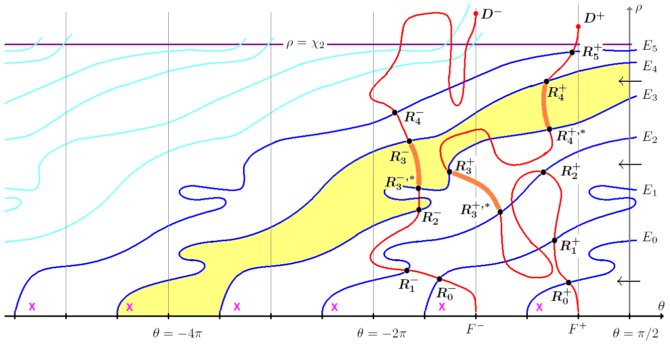
Refer to caption

Figure 4: The figure shows, in the case N=2N=2, the intersections 𝑹𝒌±\boldsymbol{R^{\pm}_{k}} and 𝑹𝒌±,∗\boldsymbol{R^{\pm,*}_{k}} between F±​(τ)F^{\pm}(\tau) and Ek​(τ)E_{k}(\tau), when τ>τN=2\tau>\tau_{N=2}. Some of the 𝑹𝒌±,∗\boldsymbol{R^{\pm,*}_{k}} coincide with 𝑹𝒌−𝟏±\boldsymbol{R^{\pm}_{k-1}}. When 𝑹𝒌±,∗≠𝑹𝒌−𝟏±\boldsymbol{R^{\pm,*}_{k}}\neq\boldsymbol{R^{\pm}_{k-1}} we have thickened the paths ak±​(τ)a_{k}^{\pm}(\tau) corresponding to slow decay solution. Condition (3.8) provides a control on the corresponding trajectories Ω⁡(t,τ,Ω¯)\Omega(t,\tau,\bar{\Omega}) which cannot pass the line θ=π/2\theta=\pi/2 from the left to the right. Moreover such solutions remain in Γk​(t)∖Γk−1​(t)\Gamma_{k}(t)\setminus\Gamma_{k-1}(t) for every t>τt>\tau, and converge to the switched polar coordinates of 𝑷±\boldsymbol{P^{\pm}} denoted in the figure by x. We have dropped the “(τ)(\tau)” for major clarity.

3.3 The existence of regular slow decay solutions

We focus now our attention on the existence of slow decay solutions following the arguments presented in [11, 20].

In the previous section, we have proved that F±​(τ)F^{\pm}(\tau) leaves Γk​(τ)\Gamma_{k}(\tau) in some points 𝑹𝒌±​(τ)\boldsymbol{R_{k}^{\pm}}(\tau). In Figure 3, a simple situation is pictured: the intersections F±​(τ)∩Ek​(τ)F^{\pm}(\tau)\cap E_{k}(\tau) consist of a unique point. Unfortunately, we cannot prove in general such a uniqueness property. Indeed, a more complex situation can arise: the intersections F±​(τ)∩Γk​(τ)F^{\pm}(\tau)\cap\Gamma_{k}(\tau) can consist of many disconnected paths, as in Figure 4. However, from (3.11), there exists necessarily at least one sub-path of F±​(τ)F^{\pm}(\tau) linking Ek−1​(τ)E_{k-1}(\tau) to Ek​(τ)E_{k}(\tau).

Hence, once fixed an integer NN and τ>τN\tau>\tau_{N} as above, for every integer k∈(0,2N+1]k\in(0,2N+1], we can find Ak∗∈[Ak−1,Ak)A_{k}^{*}\in[A_{k-1},A_{k}) such that

Ak∗:=max⁡{d∈[0,Ak):exists ​L>0​ such that ​Ωlu,+​(d,τ)=Ωl,k−1s​(L,τ)}.A_{k}^{*}:=\max\{d\in[0,A_{k})\,:\,\text{exists }L>0\text{ such that }\Omega^{u,+}_{l}(d,\tau)=\Omega^{s}_{l,k-1}(L,\tau)\}\,.

Set 𝑹𝒌+,∗:=Ωlu,+​(Ak∗,τ)\boldsymbol{R^{+,*}_{k}}:=\Omega^{u,+}_{l}(A_{k}^{*},\tau) and ak+​(τ):={Ωlu,+​(d,τ):d∈(Ak∗,Ak)}a_{k}^{+}(\tau):=\{\Omega^{u,+}_{l}(d,\tau)\,:\,d\in(A_{k}^{*},A_{k})\}. Then ak+​(τ)⊂Γk​(τ)∖Γk−1​(τ)a_{k}^{+}(\tau)\subset\Gamma_{k}(\tau)\setminus\Gamma_{k-1}(\tau) (see Figure 4). Similarly, for every integer k∈(0,2​N]k\in(0,2N], we can find Bk∗∈[Bk−1,Bk)B_{k}^{*}\in[B_{k-1},B_{k}) such that

Bk∗:=max⁡{d∈[0,Bk):exists ​L>0​ such that ​Ωlu,−​(d,τ)=Ωl,ks​(L,τ)}.B_{k}^{*}:=\max\{d\in[0,B_{k})\,:\,\text{exists }L>0\text{ such that }\Omega^{u,-}_{l}(d,\tau)=\Omega^{s}_{l,k}(L,\tau)\}\,.

Correspondingly, define 𝑹𝒌−,∗:=Ωlu,−​(Bk∗,τ)\boldsymbol{R^{-,*}_{k}}:=\Omega^{u,-}_{l}(B_{k}^{*},\tau) and ak−​(τ):={Ωlu,−​(d,τ):d∈(Bk∗,Bk)}⊂Γk+1​(τ)∖Γk​(τ)a_{k}^{-}(\tau):=\{\Omega^{u,-}_{l}(d,\tau)\,:\,d\in(B_{k}^{*},B_{k})\}\subset\Gamma_{k+1}(\tau)\setminus\Gamma_{k}(\tau).

Possibly we can have Ak∗=Ak−1A_{k}^{*}=A_{k-1} or Bk∗=Bk−1B_{k}^{*}=B_{k-1} for some kk’s (in the simple situation presented in Figure 3, they hold for every kk).

3.6 Lemma.

For every d∈(Ak∗,Ak)d\in(A_{k}^{*},A_{k}), u⁡(r,d)u(r,d) is a regular slow decay solution. Similarly, for every d∈(Bk∗,Bk)d\in(B_{k}^{*},B_{k}), u⁡(r,−d)u(r,-d) is a regular slow decay solution.

Proof.

By Lemma 2.6, we need to prove that 𝒙𝒍​(t,τ,𝑸)→𝑷+\boldsymbol{x_{l}}(t,\tau,{\boldsymbol{Q}})\to\boldsymbol{P^{+}} or 𝒙𝒍​(t,τ,𝑸)→𝑷−\boldsymbol{x_{l}}(t,\tau,{\boldsymbol{Q}})\to\boldsymbol{P^{-}} as t→+∞t\to+\infty, where 𝑸=Σlu,+​(d,τ){\boldsymbol{Q}}=\Sigma^{u,+}_{l}(d,\tau).

For every 𝑸∈ℝ2{\boldsymbol{Q}}\in\mathbb{R}^{2}, let us denote by Ω⁡(t,τ,Ω𝑸)\Omega(t,\tau,\Omega_{\boldsymbol{Q}}) the trajectory of 𝒙𝒍​(t,τ,𝑸)\boldsymbol{x_{l}}(t,\tau,{\boldsymbol{Q}}) in the stripe 𝒮\mathcal{S}, where Ω𝑸=(ϕ𝑸,ρ𝑸)∈𝒮\Omega_{\boldsymbol{Q}}=(\phi_{\boldsymbol{Q}},\rho_{\boldsymbol{Q}})\in\mathcal{S} corresponds to the switched polar coordinates of 𝑸{\boldsymbol{Q}}, i.e. 𝑸=ρ𝑸​(cos⁡ϕ𝑸,sin⁡ϕ𝑸){\boldsymbol{Q}}=\rho_{\boldsymbol{Q}}(\cos\phi_{\boldsymbol{Q}},\sin\phi_{\boldsymbol{Q}}). Notice that

Ω𝑸∈Ek​(τ)⇒Ω⁡(t,τ,Ω𝑸)∈Ek​(t)​∀t∈ℝ,Ω𝑸∉Ek​(τ)⇒Ω⁡(t,τ,Ω𝑸)∉Ek​(t)​∀t∈ℝ,Ω𝑸∈F±​(τ)⇒Ω⁡(t,τ,Ω𝑸)∈F±​(t)​∀t∈ℝ,Ω𝑸∉F±​(τ)⇒Ω⁡(t,τ,Ω𝑸)∉F±​(t)​∀t∈ℝ.\begin{array}[]{l}\Omega_{\boldsymbol{Q}}\in E_{k}(\tau)\Rightarrow\Omega(t,\tau,\Omega_{\boldsymbol{Q}})\in E_{k}(t)\ \forall t\in\mathbb{R}\,,\\ \Omega_{\boldsymbol{Q}}\notin E_{k}(\tau)\Rightarrow\Omega(t,\tau,\Omega_{\boldsymbol{Q}})\notin E_{k}(t)\ \forall t\in\mathbb{R}\,,\\ \Omega_{\boldsymbol{Q}}\in F^{\pm}(\tau)\Rightarrow\Omega(t,\tau,\Omega_{\boldsymbol{Q}})\in F^{\pm}(t)\ \forall t\in\mathbb{R}\,,\\ \Omega_{\boldsymbol{Q}}\notin F^{\pm}(\tau)\Rightarrow\Omega(t,\tau,\Omega_{\boldsymbol{Q}})\notin F^{\pm}(t)\ \forall t\in\mathbb{R}\,.\\ \end{array} (3.12)

Indeed, they correspond to the sets Wls,±​(τ)W^{s,\pm}_{l}(\tau) and Wlu,±​(τ)W^{u,\pm}_{l}(\tau), which satisfy the same property, cf. (2.8) and (2.9).

By (3.8), the flow on {θ=π/2}⊂𝒮\{\theta=\pi/2\}\subset\mathcal{S} points towards {θ<π/2}\{\theta<\pi/2\}. Hence, using also (3.12), we see that if Ω𝑸∈Γk​(τ)∖Γk−1​(τ)\Omega_{\boldsymbol{Q}}\in\Gamma_{k}(\tau)\setminus\Gamma_{k-1}(\tau) then Ω⁡(t,τ,Ω𝑸)∈Γk​(t)∖Γk−1​(t)\Omega(t,\tau,\Omega_{\boldsymbol{Q}})\in\Gamma_{k}(t)\setminus\Gamma_{k-1}(t) for every t>τt>\tau. Moreover, since Wls​(t)→Wls​(+∞)W_{l}^{s}(t)\to W_{l}^{s}(+\infty), we have that Ek​(t)→Ek​(+∞)E_{k}(t)\to E_{k}(+\infty), where Ek​(+∞)E_{k}(+\infty) corresponds to a polar representation of a subset of Ws​(+∞)W^{s}(+\infty). In particular Γk​(t)∖Γk−1​(t)\Gamma_{k}(t)\setminus\Gamma_{k-1}(t) remains bounded and Γk​(t)∖Γk−1​(t)→Γk​(+∞)∖Γk−1​(+∞)\Gamma_{k}(t)\setminus\Gamma_{k-1}(t)\to\Gamma_{k}(+\infty)\setminus\Gamma_{k-1}(+\infty), where Γj​(+∞)\Gamma_{j}(+\infty) is the region enclosed by Ej​(+∞)E_{j}(+\infty), θ=π/2\theta=\pi/2 and ρ=0\rho=0.

We introduce the polar coordinates of the non-trivial critical points 𝑷±=ρ±​(cos⁡ϕ±,sin⁡ϕ±)\boldsymbol{P^{\pm}}=\rho_{\pm}(\cos\phi_{\pm},\sin\phi_{\pm}) and the corresponding points Ω𝑷,2​j=(ϕ+−2​π​j,ρ+)\Omega_{\boldsymbol{P},2j}=(\phi_{+}-2\pi j,\rho_{+}) and Ω𝑷,2​j+1=(ϕ−−2​π​j,ρ−)\Omega_{\boldsymbol{P},2j+1}=(\phi_{-}-2\pi j,\rho_{-}) on the stripe 𝒮\mathcal{S}. The unique attractor of Γk​(+∞)∖Γk−1​(+∞)\Gamma_{k}(+\infty)\setminus\Gamma_{k-1}(+\infty) is Ω𝑷,k\Omega_{\boldsymbol{P},k}, so we have Ω⁡(t,τ,Ω𝑸)→Ω𝑷,k\Omega(t,\tau,\Omega_{\boldsymbol{Q}})\to\Omega_{\boldsymbol{P},k} as t→+∞t\to+\infty for every Ω𝑸∈Γk​(τ)∖Γk−1​(τ)\Omega_{\boldsymbol{Q}}\in\Gamma_{k}(\tau)\setminus\Gamma_{k-1}(\tau). The previous limits corresponds to 𝒙𝒍​(t,τ,𝑸)→𝑷+\boldsymbol{x_{l}}(t,\tau,{\boldsymbol{Q}})\to\boldsymbol{P^{+}} for kk even and to 𝒙𝒍​(t,τ,𝑸)→𝑷−\boldsymbol{x_{l}}(t,\tau,{\boldsymbol{Q}})\to\boldsymbol{P^{-}} for kk odd. Hence, the corresponding solution has a slow decay, cf. Remark 2.6. Choosing Ω𝑸=Ωlu,±​(d,τ)∈ak±​(τ)\Omega_{\boldsymbol{Q}}=\Omega^{u,\pm}_{l}(d,\tau)\in a_{k}^{\pm}(\tau) we find a regular slow decay solution u⁡(r,±d)u(r,\pm d). ∎

As a consequence of the previous argument, we also have the following lemma.

3.7 Lemma.

For every d∈(Ak∗,Ak]d\in(A_{k}^{*},A_{k}], u⁡(r,d)u(r,d) satisfies −d−<u⁡(r,d)<d+-d^{-}<u(r,d)<d^{+} for every r>eτNr>{\rm e}^{\tau_{N}}. Similarly, for every d∈(Bk∗,Bk]d\in(B_{k}^{*},B_{k}], u⁡(r,−d)u(r,-d) satisfies −d−<u⁡(r,−d)<d+-d^{-}<u(r,-d)<d^{+} for every r>eτNr>{\rm e}^{\tau_{N}}.

Proof.

For every τ>τN\tau>\tau_{N} we have F±​(τ)⊂ℝ×[0,χN]F^{\pm}(\tau)\subset\mathbb{R}\times[0,\chi_{N}]. So, by (3.10), we have ρlu,±​(d,τ)<d±​eαl​τ\rho_{l}^{u,\pm}(d,\tau)<d^{\pm}\,{\rm e}^{\alpha_{l}\tau}. Consequently, −d−<xl​(t,τ,Σlu,±​(d,τ))​e−αl​t<d+-d^{-}<x_{l}(t,\tau,\Sigma_{l}^{u,\pm}(d,\tau)){\rm e}^{-\alpha_{l}t}<d^{+} for every τ>τN\tau>\tau_{N} and the assertion follows. ∎

3.4 The number of non-degenerate zeros

The correct estimates on the number of nondegenerate zeros of the fast decay solutions is given by the following lemma, see e.g. [11, Lemma 3.3] (see also [3, 18, 20] for a full fledged proof).

3.8 Lemma.

Let us consider system ( S l ) and assume 𝐇𝐮\boldsymbol{H^{u}} . Consider the trajectory 𝐱𝐥​(⋅,τ,𝐐)\boldsymbol{x_{l}}(\cdot,\tau,{\boldsymbol{Q}}) with 𝐐=Σlu,+​(d,τ){\boldsymbol{Q}}=\Sigma^{u,+}_{l}(d,\tau) and its polar coordinates (2.12). Then, the angle ϑ:=θlu,+​(d,τ)−θlu,+​(0,τ)=θlu,+​(d,τ)\vartheta:=\theta^{u,+}_{l}(d,\tau)-\theta^{u,+}_{l}(0,\tau)=\theta^{u,+}_{l}(d,\tau) performed by the unstable manifold Wlu,+​(τ)W_{l}^{u,+}(\tau) equals the angle ϕ:=ϕl​(t,τ,𝐐)−ϕl​(−∞,τ,𝐐)\phi:=\phi_{l}(t,\tau,{\boldsymbol{Q}})-\phi_{l}(-\infty,\tau,{\boldsymbol{Q}}) performed by the trajectory 𝐱𝐥​(t,τ,𝐐)\boldsymbol{x_{l}}(t,\tau,{\boldsymbol{Q}}) in the interval (−∞,τ](-\infty,\tau].

Similarly, assume 𝐇𝐬\boldsymbol{H^{s}} and consider 𝐱𝐥​(⋅,τ,𝐐)\boldsymbol{x_{l}}(\cdot,\tau,{\boldsymbol{Q}}) with 𝐐=Σls,+​(L,τ){\boldsymbol{Q}}=\Sigma^{s,+}_{l}(L,\tau). Then, the angle ϑ:=θls,+​(L,τ)−θls,+​(0,τ)=θls,+​(L,τ)+π/2\vartheta:=\theta^{s,+}_{l}(L,\tau)-\theta^{s,+}_{l}(0,\tau)=\theta^{s,+}_{l}(L,\tau)+\pi/2 performed by the stable manifold Wls,+​(τ)W_{l}^{s,+}(\tau) equals, but with reversed sign, the angle φ:=ϕl​(+∞,τ,𝐐)−ϕl​(τ,τ,𝐐)\varphi:=\phi_{l}(+\infty,\tau,{\boldsymbol{Q}})-\phi_{l}(\tau,\tau,{\boldsymbol{Q}}) performed by the trajectory 𝐱𝐥​(t,τ,𝐐)\boldsymbol{x_{l}}(t,\tau,{\boldsymbol{Q}}) in the interval [τ,+∞)[\tau,+\infty).

A similar reasoning holds for 𝐐=Σlu,−​(d,τ){\boldsymbol{Q}}=\Sigma^{u,-}_{l}(d,\tau) and 𝐐=Σls,−​(L,τ){\boldsymbol{Q}}=\Sigma^{s,-}_{l}(L,\tau).

The previous lemma is the key point in order to prove the nodal properties of the regular solutions we have found.

Let us start with regular fast decay ones. We consider u⁡(r,Ak)u(r,A_{k}) and the associated points 𝑸𝒌+=Σlu,+​(Ak,τ)∈ℝ2\boldsymbol{Q^{+}_{k}}=\Sigma^{u,+}_{l}(A_{k},\tau)\in\mathbb{R}^{2} and 𝑹𝒌+=Ωlu,+​(Ak,τ)∈𝒮\boldsymbol{R^{+}_{k}}=\Omega^{u,+}_{l}(A_{k},\tau)\in\mathcal{S}. By the previous lemma, in order to obtain the angle performed by 𝒙𝒍​(⋅,τ,𝑸𝒌+)\boldsymbol{x_{l}}(\cdot,\tau,\boldsymbol{Q^{+}_{k}}) in the whole time interval (−∞,+∞)(-\infty,+\infty) we have to consider the angle variation along the path F+​(τ)F^{+}(\tau) between (0,0)∈𝒮(0,0)\in\mathcal{S} and 𝑹𝒌+\boldsymbol{R^{+}_{k}} and then the one along Ek​(τ)E_{k}(\tau) between 𝑹𝒌+\boldsymbol{R^{+}_{k}} and (−π⁡(k+1/2),0)∈𝒮(-\pi(k+1/2),0)\in\mathcal{S}. We easily obtain a tolal angle of −π⁡(k+1/2)-\pi(k+1/2). So, by the flow condition (3.8), the trajectory Ω⁡(⋅,τ,𝑹𝒌+)\Omega(\cdot,\tau,\boldsymbol{R^{+}_{k}}) intersects the vertical lines θ=−π/2−jπ\theta=-\pi/2-j\pi once for every integer j∈{1,…,k}j\in\{1,\ldots,k\}, thus finding exactly kk zeros of 𝒙𝒍​(⋅,τ,𝑸𝒌+)\boldsymbol{x_{l}}(\cdot,\tau,\boldsymbol{Q^{+}_{k}}) which are non-degenerate. A similar reasoning holds for u⁡(r,−Bk)u(r,-B_{k}).

We turn now to consider u⁡(r,d)u(r,d) with d∈(Ak∗,Ak)d\in(A^{*}_{k},A_{k}) and, correspondingly, 𝑸=Σlu,+​(d,τ){\boldsymbol{Q}}=\Sigma^{u,+}_{l}(d,\tau) and 𝑹=Ωlu,+​(d,τ){\boldsymbol{R}}=\Omega^{u,+}_{l}(d,\tau). The total angle performed by the solution 𝒙𝒍​(⋅,τ,𝑸)\boldsymbol{x_{l}}(\cdot,\tau,{\boldsymbol{Q}}) in the time interval (−∞,τ)(-\infty,\tau) is given by the angle variation along the path F+​(τ)F^{+}(\tau). Then, for every t>τt>\tau, Ω⁡(t,τ,𝑹)\Omega(t,\tau,{\boldsymbol{R}}) is forced to remain between the paths Ek−1​(t)E_{k-1}(t) and Ek​(t)E_{k}(t) and to converge to Ω𝑷,k\Omega_{\boldsymbol{P},k} as t→+∞t\to+\infty: thus the total angle variation is −2​j​π+ϕ+∈(−(2​j+1)​π,−2​j​π)-2j\pi+\phi_{+}\in(-(2j+1)\pi,-2j\pi) if k=2​jk=2j, resp −2​j​π+ϕ−∈(−(2​j+2)​π,−(2​j+1)​π)-2j\pi+\phi_{-}\in(-(2j+2)\pi,-(2j+1)\pi) if k=2​j+1k=2j+1. By (3.8), the trajectory Ω⁡(⋅,τ,𝑹)\Omega(\cdot,\tau,\boldsymbol{R}) intersects all the lines θ=−π/2−jπ\theta=-\pi/2-j\pi only once and correspondingly all the zeros are non-degenerate. A similar reasoning holds for u⁡(r,−d)u(r,-d) with d∈(Bk∗,Bk)d\in(B^{*}_{k},B_{k}).

3.5 Back to the orginal problem

We have proved Theorem 1.1 for the differential equation (1.1) with ff replaced by its truncation f¯\bar{f} introduced in (3.1). We are going now to prove that such solutions solve also the original equation (1.1). To this aim we need Lemma 3.9 below.

We underline that it is well-known in literature that, under hypotheses (F) and (K), a positive solution of (1.2) with u⁡(0)<d+u(0)<d^{+} necessarily satisfies u⁡(r)<d+u(r)<d^{+} for every r>0r>0 (and correspondingly negative ones with u⁡(0)>−d−u(0)>-d^{-} satisfy u⁡(r)>−d−u(r)>-d^{-}). The situation is more complicated if we treat nodal solutions. In the case of a decreasing weight kk, we can easily provide the same a priori estimate by introducing an energy function.

For a more general weight kk, such a situation is not ensured and we argue as follows.

3.9 Lemma.

Consider 𝐐=(Qx,Qy)∈ℝ2{\boldsymbol{Q}}=(Q_{x},Q_{y})\in\mathbb{R}^{2} with −d−<Qx​e−αl​σ<d+-d^{-}<Q_{x}{\rm e}^{-\alpha_{l}\sigma}<d^{+} for a certain σ\sigma. Suppose that there exists σ′>σ\sigma^{\prime}>\sigma such that 𝐱𝐥​(σ′,σ,𝐐)\boldsymbol{x_{l}}(\sigma^{\prime},\sigma,{\boldsymbol{Q}}) satisfies −d−<xl​(σ′,σ,𝐐)​e−αl​σ′<d+-d^{-}<x_{l}(\sigma^{\prime},\sigma,{\boldsymbol{Q}}){\rm e}^{-\alpha_{l}\sigma^{\prime}}<d^{+}. Then, the solution 𝐱𝐥​(t,σ,𝐐)\boldsymbol{x_{l}}(t,\sigma,{\boldsymbol{Q}}) of ( S l ), with glg_{l} as in (3.3), satisfies −d−<xl​(t,σ,𝐐)​e−αl​t<d+-d^{-}<x_{l}(t,\sigma,{\boldsymbol{Q}}){\rm e}^{-\alpha_{l}t}<d^{+}, for every t∈(σ,σ′)t\in(\sigma,\sigma^{\prime}).

Proof.

Defining ξl​(t)=xl​(t)−d+​eαl​t\xi_{l}(t)=x_{l}(t)-d^{+}{\rm e}^{\alpha_{l}t} we obtain the system

{ξ˙l=αl​ξl+yl​|yl|2−pp−1y˙l=γl​yl−hl​(t,ξl)\begin{cases}\dot{\xi}_{l}=\alpha_{l}\xi_{l}+y_{l}|y_{l}|^{\frac{2-p}{p-1}}\\ \dot{y}_{l}=\gamma_{l}y_{l}-h_{l}(t,\xi_{l})\end{cases} (3.13)

where hl​(t,ξl)=gl​(t,ξl+d+​eαl​t)h_{l}(t,\xi_{l})=g_{l}(t,\xi_{l}+d^{+}{\rm e}^{\alpha_{l}t}). Notice that, by (3.3), hl​(t,ξl)≤0h_{l}(t,\xi_{l})\leq 0 if ξl>0\xi_{l}>0. Moreover, as in (3.8),

ξ˙l​(t)​y​(t)>0​ whenever ​ξl​(t)=0​ and ​yl​(t)≠0,\dot{\xi}_{l}(t)y(t)>0\text{ whenever }\xi_{l}(t)=0\text{ and }y_{l}(t)\neq 0\,, (3.14)

In particular 𝒬1={(ξ,y):ξ≥0,y≥0}\mathcal{Q}_{1}=\{(\xi,y)\,:\,\xi\geq 0\,,y\geq 0\} and 𝒬2={(ξ,y):ξ≥0,y≤0}\mathcal{Q}_{2}=\{(\xi,y)\,:\,\xi\geq 0\,,y\leq 0\} are respectively positively and negatively invariant sets.

In this setting we have to prove that if a solution (ξl​(t),yl​(t))(\xi_{l}(t),y_{l}(t)) of (3.13) satisfies ξl​(σ)<0\xi_{l}(\sigma)<0 and ξl​(σ′)<0\xi_{l}(\sigma^{\prime})<0 then ξl​(t)<0\xi_{l}(t)<0 for every t∈(σ,σ′)t\in(\sigma,\sigma^{\prime}). Arguing by contradiction, let t0∈(σ,σ′)t_{0}\in(\sigma,\sigma^{\prime}) be such that ξl​(t0)≥0\xi_{l}(t_{0})\geq 0. If yl​(t0)≥0y_{l}(t_{0})\geq 0 then (ξl​(t0),yl​(t0))∈𝒬1(\xi_{l}(t_{0}),y_{l}(t_{0}))\in\mathcal{Q}_{1} which is invariant in the future and we get a contradiction with ξl​(σ′)<0\xi_{l}(\sigma^{\prime})<0. Conversely, if yl​(t0)<0y_{l}(t_{0})<0 then (ξl​(t0),yl​(t0))∈𝒬2(\xi_{l}(t_{0}),y_{l}(t_{0}))\in\mathcal{Q}_{2} which is invariant in the past and we get a contradiction with ξl​(σ)<0\xi_{l}(\sigma)<0.

The estimates with respect d−d^{-} is analogous. ∎

We consider a regular solution u⁡(r,d)u(r,d) of (1.2) with f=f¯f=\bar{f} as in (3.1) and the corresponding solution 𝒙𝒍\boldsymbol{x_{l}} of system ( S l ) (notice that glg_{l} is as in (3.3)).

If d∈(−d−,d+)d\in(-d^{-},d^{+}), by (3.4), we have u⁡(r,d)∈(−d−,d+)u(r,d)\in(-d^{-},d^{+}) for every r∈[0,et1]r\in[0,{\rm e}^{t_{1}}], with et1{\rm e}^{t_{1}} sufficiently small. Hence, we have −d−<xl​(t)​e−αl​t<d+-d^{-}<x_{l}(t){\rm e}^{-\alpha_{l}t}<d^{+} for every t≤t1t\leq t_{1}.

Now, given a regular solution u⁡(r,d)u(r,d) with d∈(Ak∗,Ak]d\in(A_{k}^{*},A_{k}], setting N>k/2N>k/2 and 𝑸=Σlu,+​(d,τ){\boldsymbol{Q}}=\Sigma_{l}^{u,+}(d,\tau), by Lemma 3.7, we have −d−<xl​(t,τ,𝑸)​e−αl​t<d+-d^{-}<x_{l}(t,\tau,{\boldsymbol{Q}}){\rm e}^{-\alpha_{l}t}<d^{+} for every t≥τ>τNt\geq\tau>\tau_{N}.

So, we can apply Lemma 3.9 with σ=t1\sigma=t_{1} and σ′=τ>τN\sigma^{\prime}=\tau>\tau_{N}, thus obtaining −d−<xl​(t,τ,𝑸)​e−αl​t<d+-d^{-}<x_{l}(t,\tau,{\boldsymbol{Q}}){\rm e}^{-\alpha_{l}t}<d^{+} for every t∈[t1,τ]t\in[t_{1},\tau]. Summing up, the previous estimate holds for every t∈ℝt\in\mathbb{R}.

The same reasoning can be adapted to the case of a regular slow decay solution u⁡(r,−d)u(r,-d) with d∈(Bk∗,Bk]d\in(B_{k}^{*},B_{k}].

Hence, the previously found solutions solve indeed the original equation and the proof of Theorem 1.1 is thus completed.

References

  • [1] B. Acciaio and P. Pucci, Existence of radial solutions for quasilinear elliptic equations with singular nonlinearities, Adv. Nonlinear. Stud. 3 (2003), 513–541.
  • [2] S. Alarcón and A. Quaas, Large number of fast decay ground states to Matukuma-type equations, J. Differential Equations 248 (2010), 866–892.
  • [3] R. Bamon, I. Flores and M. del Pino, Ground states of semilinear elliptic equations: a geometric approach, Ann. Inst. H. Poincaré Anal. Non Linéaire 17 (2000), 551–581.
  • [4] V. Barutello, S. Secchi and E. Serra, A note on the radial solutions for the supercritical Hénon equation, J. Math. Anal. Appl. 341 (2008), 720–728.
  • [5] M.F. Bidaut-Vèron, Local and global behavior of solutions of quasilinear equations of Emden-Fowler type, Arch. Ration. Mech. Anal. 107 (1989) 293–324.
  • [6] J. Byeon and Z.-Q- Wang, On the Hénon equation: asymptotic profile of ground states, Ann. Instit. H. Poincaré Anal. Non Linéaire 23 (2006), 803–828.
  • [7] E. Coddington and N. Levinson, Theory of Ordinary Differential Equations, Mc Graw Hill, New York, 1955.
  • [8] C. Cortázar, J. Dolbeault, M. García-Huidobro and R. Manásevich, Existence of sign-changing solutions for an equation with a weighted pp-laplace operator, Nonlinear Analysis 110 (2014), 1–22.
  • [9] C. Cortázar, M. García-Huidobro and P. Herreros, Multiplicity results for sign-changing bound state solutions of a semilinear equation, J. Differential Equations 259 (2015), 7108–7134.
  • [10] C. Cortázar, M. García-Huidobro and C.S. Yarur, On the existence of sign changing bound state solutions of a quasilinear equation, J. Differential Equations 254 (2013), 2603–2625.
  • [11] F. Dalbono and M. Franca, Nodal solutions for supercritical Laplace equations, Comm. Math. Phys. 347 (2016), 875–901.
  • [12] E.N. Dancer and Y. Du, Some remarks on Liouville type results for quasilinear elliptic equations, Proc. Amer. Math. Soc. 131 (2002), 1891–1899.
  • [13] J. Dolbeault and I. Flores, Geometry of phase space and solutions of semilinear elliptic equations in a ball, Trans. Amer. Math. Soc. 359 (2007), 4073–4087.
  • [14] P. Felmer, A. Quaas and M. Tang, On the complex structure of positive solutions to Matukuma-type equations, Ann. I. H. Poincaré 26 (2009), 869–-887.
  • [15] R.H. Fowler, Further studies of Emden’s and similar differential equations, Quart. J. Math. 2 (1931), 259–288.
  • [16] M. Franca, Fowler transformation and radial solutions for quasilinear elliptic equations. Part 2: nonlinearities of mixed type, Ann. Mat. Pura Appl. 189 (2009), 67–94.
  • [17] M. Franca, Radial ground states and singular ground states for a spatial dependent pp-Laplace equation, J. Differential Equations 248 (2010), 2629–2656
  • [18] M. Franca, Positive solutions of semilinear elliptic equations: a dynamical approach, Differential Integral Equations 26 (2013), 505–554.
  • [19] M. Franca and A. Sfecci, On a diffusion model with absorption and production, Nonlinear Anal. Real World Appl. 34 (2017), 41–60.
  • [20] M. Franca and A. Sfecci, Entire solutions of superlinear problems with indefinite weights and Hardy potentials, J. Dynam. Differential Equations (2017), 38 pages, DOI: 10.1007/s10884-017-9589-z.
  • [21] R. Johnson, Concerning a theorem of Sell, J. Differential Equations 30 (1978), 324–339.
  • [22] R. Johnson, X.B. Pan and Y.F. Yi, The Melnikov method and elliptic equation with critical exponent, Indiana Univ. Math. J. 43 (1994), 1045–1077.
  • [23] N. Kawano, E. Yanagida and S. Yotsutani, Structure theorems for positive radial solutions to d​i​v​(|D​u|m−2​D​u)+K⁡(|x|)​uq=0div(|Du|^{m-2}Du)+K(|x|)u^{q}=0 in ℝn\mathbb{R}^{n}, J. Math. Soc. Japan 45 (1993), 719-742.
  • [24] M.K. Kwong, J.B. McLeod, L.A. Peletier and W.C. Troy, On ground state solutions of −Δ​u=up−uq-\Delta u=u^{p}-u^{q}, J. Differential Equations 95 (1992), 218–239.
  • [25] W.-M. Ni, A nonlinear Dirichlet problem on the unit ball and its applications, Indiana Univ. Math. J. 31 (1982), 801–807.
  • [26] J. Serrin and M. Tang, Uniqueness of ground states for quasilinear elliptic equations, Indiana Univ. Math. J. 49 (2000) 897–923.
  • [27] M. Tang, Existence and uniqueness of fast decay entire solutions of quasilinear elliptic equations, J. Differential Equations 164 (2000), 155–179.
  • [28] M. Tang, Uniqueness and global structure of positive radial solutions for quasilinear elliptic equations, Comm. Partial Differential Equations 26 (2001), 909–938.