Analysis of etching at a solid-solid interface
Abstract
We present a method to derive an analytical expression for the roughness of an eroded surface whose dynamics are ruled by cellular automaton. Starting from the automaton, we obtain the time evolution of the height average and height variance (roughness).
We apply this method to the etching model in dimensions, and then we obtain the roughness exponent. Using this in conjunction with the Galilean Invariance we obtain the other exponents, which perfectly match the numerical results obtained from simulations. These exponents are exact and they are the same as those exhibited by the Kardar-Parisi-Zhang (KPZ) model for this dimension. Therefore, our results provide proof for the conjecture that the etching and KPZ models belong to the same universality class. Moreover, the method is general, and it can be applied to other cellular automata models.
Phys. Rev. E 94, 042119 – Published 17 October 2016
DOI: 10.1103/PhysRevE.94.042119
pacs
68.35.Ct, 05.45.Df, 05.40.-a, 05.90.+mI Introduction
The dynamics of growth interfaces has become an interdisciplinary field and has had large success in the unification of concepts in many branches, ranging from applications in materials science [Yin05, Renner06] to fundamental problems in mathematics [Hairer13]. In the last decades two different approaches have been widely used. The first is the use of differential stochastic equations such as the KPZ equation [Kardar86, Hairer13, Sasamoto10]. However, many recent advances are due to the availability of fast and affordable computer clusters. Such development has made it feasible, for instance, to obtain numerical simulations of large particle systems by obeying simple repetitive rules which mimic complex systems and whose emergent information and properties have been obtained through several techniques and approaches. The second method is defined as a cellular automata analysis. It is obvious that there is a need to connect these methods, and considerable effort has been exerted to achieve this goal. In this work we obtain the first exact solution for a growth cellular automaton model, i.e., we obtain the exact exponents for the etching model, and we show that it belongs to the same class of universality as that of the KPZ model.
The surface growth phenomenon, when treated as a stochastic process, encompass a wide field of applications. Some examples of growth systems are corrosion [Mello01, Renner06, Reis03, Rodrigues15], fire propagation [Merikoski03], atomic deposition [Csahok92], evolution of bacterial colonies [Ben-Jacob94, Matsushita90], and spherical models [Henkel15]. Models have been proposed and studied through experiments [Ben-Jacob94, Matsushita90], analytical calculations [Barabasi95] and computational simulations [Mello01, Reis03].
Surfaces with different internal dynamics can lead to distinct profiles, which can be characterized by different measures, the most important being the mean value and the standard deviation of the surface height , . When related to surfaces, the standard deviation is often called the surface width or roughness, and is defined as
| (1) |
wherein the variable ,
| (2) |
measures how high a site is with respect to the mean substrate height
| (3) |
Though the average height increases continuously due to the growth process, the dynamic equilibrium leads to surface width saturation after a period of roughening buildup. The saturated surface width, , is often expresed as a function of the substrate size as the power law , being the roughness exponent. The saturation occurs at times larger than a characteristic time that follows the power law , where is the dynamic exponent. Before saturation (), evolves as a power law with the growth exponent , .
In the literature, we can find good examples of cellular automata models [Katzav04, Predota96, Chua05, Buceta14] whose continuous versions are similar to the KPZ equation. Although many works were dedicated at obtaining the exponents, little effort was directed into obtaining a relation to describe the roughness time evolution. In this work we develop a general method to obtain the roughness evolution for cellular automata models. Then we apply the method to the etching model [Mello01]. We exactly obtain the saturated roughness and the roughness exponent . From this we obtain and , and we show that the etching model belongs to the same class of universality as that of the KPZ model.
II Basic theory
We develop here the basic ideas to obtain the roughness for a cellular automaton model. The details are left to the appendix. Consider the variation of roughness squared for a given time interval as
| (4) |
Here is the variation in one possible event, i.e., we take a large number of experiments and at a time we take a variation that occurs in the next time interval. This process is equivalent to being weighted by the probability distribution , which depends on the configuration at the site , its neighbors , and time. Note that values of are discrete variables. However, when we average over a large number of experiments all possible real values of arise, and we can define the probability and as continuous functions.
Unfortunately, there is no theory which can be used to obtain . In this way we define the auxiliary function
| (5) |
which we will call the evolution factor. Here, is an equiprobability distribution. The integral on the denominator can be solved exactly. With this definition we rewrite Eq. (4) as
| (6) |
We note that Eq. (6) is the same as Eq. (4), and no approximation were applied. The evolution factor contains all information about the dynamics and correlation. It makes it possible to separate the time integral from the integral in the configuration space. In this way the last integral in Eq. (6) can be exactly calculated. The factor will be discussed later for the etching model.
II.1 The equiprobability of the configurations
To make the notation less clumsy, the random site will be chosen to be , implying that only the sites are relevant. Therefore, each step of the cellular automaton changes the value of the squared surface width by .
Before proposing an expression such as we must remember that there is a finite number of substrate configurations allowed by each value of . This finite number is the result of the restrictions on imposed by the definitions of and in Equations (1) and (2),
| (7a) | ||||
| (7b) | ||||
Eq. (7a) defines the surface of a hypersphere centered at the origin and of total radius , and Eq. (7b) defines a hyperplane, which passes at the origin, both in -D, i.e., in a space of dimensions. From the intersection of these two subspaces, a spherical surface results, which is ()-D, and has the same radius .
For each combination of , , and , i.e., fixed values of these variables, the remaining ’s obeys
| (8a) | ||||
| (8b) | ||||
and forms another spherical surface, now with the dimensions . While the ()-D surface corresponds to all possible surface configurations of a given value of , the ()-D surface is the subset of these configurations defined by the triad , , and . Following a common convention for the number of accessible states, these surfaces will be called, respectively, and . Consequently, the probability of a given triad is
| (9) |
It is important to stress that the equiprobability assumption disregards the different probabilities of each configuration generated by the cellular automaton, and even the fact that some configurations are never generated for certain automata. These selections rules are due to the cellular automaton and affect the function . However, one should always bear in mind that all accessible states of a system, as defined by Eq. (7), have equal probabilities as established by Statistical Mechanics. A good test to check if the equiprobability distribution is suitable to describe the dynamics in a certain region is to observe if the behavior of is correct. If it is constant in a given region, then equiprobability is present.
Eq. (9) can be rewritten by substituting the expression for the area of a hypersphere,
| (10) |
where and are the radius of the corresponding hyperspheres and
| (11) |
where is the gamma function.
To obtain the radius we have to diagonalize the reduced hypersphereas shown in the Appendix. The above probability can than be expressed more conveniently using the coordinates
| (12) |
with the variables defined in the intervals
| (13) |
After diagonalizing the small hypersphere (see Appendix), we arrive at
| (14) |
Note that Eq. (23) and the above result are general, and consequently do not depend on of the cellular automaton used. However to obtain an explicit final result we need to select a model. In the next section we obtain this integral for the etching model
III The etching model
The etching model [Mello01] is an automaton that mimics the erosion of a surface by an acid. We randomly choose a site , and we look at its nearest neighbor. If , it is reduced to the same height as , i.e., the height of the surface decreases at each step. We then defined it using the rules:
1. Randomly choose a site .
2. If do .
3. If do .
4. Do
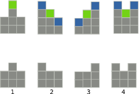
The algorithm implements a cell removal probability that is proportional to the number of the exposed faces of the cell, a reasonable approximation of the etching process. It could also describe a deposition where each exposed face has the same attachment probability. For that reason, it can be referred to as either particle removal, or deposition with . The roughness is invariant to the symmetry operation . In Fig. 1 we show the evolution for the etching model.
| Case | Limits | |||||
|---|---|---|---|---|---|---|
| 1 | 0 | -1 | 0 | -1 | 1 | |
| 2 | -1 | 0 | ||||
| 3 | 0 | -1 | ||||
| 4 | -1 |
Note that the change of the roughness has the term which is identical to the nonlinear term in the KPZ equation. The scaling exponents found by Mello et al [Mello01] in dimensions were and , suggesting that the model is within the KPZ universality class (, ) . Other studies analyzed the model in and dimensions focusing on aspects such as the dynamic behavior of the roughness and comparisons with other models belonging to the KPZ universality class [Mello15, Reis03, Reis04, Reis05, Ghaisas06, Oliveira08, Forgerini09]. Some studies highlighted that the Galilean invariance (GI) breaks down in fractal dimensions [Xun12], while recent work [Rodrigues15] shows that for , integer and , the GI holds. The last work also shows that inside this limit there is no upper critical dimension. It is important to mention that there are some results showing that GI does not seem to play the relevant role usually assumed in defining the KPZ universality class [Wio10a, Wio10b]. Finally some works demonstrate applications in the comprehension of kinetic roughening at metal-electrolyte interfaces [Cordoba07]. Those works are well-performed numerical analyses and are quite precise. However, we aspire to obtain exact solutions for this model. In the appendix we obtain for the etching model. Using those results in Eq. (14), we obtain the Eq. (38) which may be rewritten as
| (15) |
where depends only on . As shown in Eq. (41) for large values of , where
| (16) |
This is the major result of our work to obtain for the exact value for for an automaton cellular model. For the etching model in dimensions it yields . We cannot at present time use our method to obtain or . Furthermore, we cannot obtain the GI . However, numerical studies had been conducted in up to dimensions for the etching model [Rodrigues15]. If we assume the GI, and use the identity we obtain and , which are the KPZ exponents. Consequently, within the GI hypothesis, we have obtained the exact exponents for the etching model, and this adds to the evidence that it belongs to the same universality class as that of KPZ.


IV The limiting behavior
In the last section we have achieved what we proposed for this work, i.e. to obtain the exact exponents for the etching model for dimensions. Nevertheless, we feel that we need to better understand the time evolution of . The evolution factor contains all of the information about the dynamics and correlation and remains to be determined. We shall discuss it in Fig. 1 and Tab. 1. Now, we solve Eq. (15), with , to obtain
| (17) |
where
| (18) |
The constant has been absorbed in the above integral. First note that we can reverse Eq. (17) to obtain
| (19) |
Since is a growing function of , is also a growing function of , which is in agreement with the fact that is always positive.
In Fig. 2 we display as function of . We obtain by averaging over numerical experiments for several values of . In Fig. 1a we show the beginning of the growth process (, and ), i.e. before the correlations become important, is a constant. For that region , which is similar to uncorrelated random walk. This is a general behavior for any growth process.
In Fig. 2b we show for large . Note that the time here is given in units of . For , correlation becomes important, and , which means that no longer grows linearly with time. Finally, for , , i.e., we have left the region where the probability distribution is changing and arrived at the region where that distribution is in the steady state, and, consequently, is constant. The straight line , i.e., the exact value for is displayed for comparison. We note that when is very close to , the fluctuations make some values of larger than and the curve loses clarity and becomes blurred. If we increase the number of experiments, we decrease the uncertainty and the linear region increases.
This shows the importance of the evolution factor and to describe the dynamics. However, they are not necessary to obtain the exponent . This limiting behavior shows that in the beginning of the growth process, where no correlations are present, is constant. Likewise, for large times, when approaches saturation, the configurations have established themselves and no longer change. Again, the equilibrium distribution perfectly describes the phenomenon. This is identical to that which happens in anomalous diffusion [Ferreira12], where we do not have to know all of the stages of the evolution but we can obtain the exact exponents for the asymptotic behavior . In this way we can obtain the exponents , and exactly, without a full knowledge of .
V Conclusions
In this work, we present a method to obtain an equation for the roughness evolution. The definition of an evolution factor allows the separation of the time integral from that of the configuration space. This space is an dimensional space formed by the heights of the eroded surface. The probability of occurrence of a given interface configuration is the ratio between the hypersphere area of that configuration and the total hypersphere area in all possible configurations. In this way the statistical average in the configuration space can be obtained. The hypersphere method has potential for application in cellular automata models which depend only on the nearest neighbors but needs to be built differently for each type of algorithm. The only restriction on the algorithm is the condition that each site affects and is only acted on and affects the nearest neighbors. A limitation of our method is that it provides exact results only at asymptotic times, neither it provide the distribution of height , but the distribution of configurations. Nevertheless, it has the advantage of being a method for cellular automaton, an area which is mainly studied by numerical tools.
We applied the method to the etching model and obtained the roughness exponent which matches exactly with the KPZ exponent. If we consider that the GI is valid, which is supported by numerical calculation [Rodrigues15], we can say that the etching model belongs to the KPZ universality class. Recently, Sasamoto and Spohn [Sasamoto10] have solved the KPZ equation for dimensions. There, they found that the probability distribution function of the height for all . In particular, they showed that on the scale , the statistics are given by the Tracy-Widom distribution [Tracy94, Fortin15]. Moreover, we can say that we have obtained the stationary solution, , of the configuration distribution for the KPZ equation. We hope that investigations of distribution evolution in a lattice[Oliveira10] can be used to obtain at lest one approximated time dependent distribution of configurations. Finally, since our method does not involve renormalization approaches, which fails for , the generalization for is possible; nevertheless, it involves hard calculations.
Acknowledgements
This work was supported by CAPES, CNPq, and FAPDF. FAO would like to thank the kind hospitality of Professor Hyunggyu Park during his visit at the Korean Institute for Advanced Study (KIAS).
Appendix A Appendix
A.1 Evolution of the quadratic roughness
The squared surface width will be affected by the value of before and after each step, for
| (20) |
with
| (21) |
From Eq. (7a) we can write
| (22) |
A convenient expression for it can be found if we substitute the identities and , and remember that for ,
| (23) |
Equation (23) is a general formula (independent of the iterative algorithm) for the increment of the squared surface width at each time step, which must be replaced in Eq. (6). In order to obtain the dynamics of a specific algorithm, it is necessary to know the values of and , which are functions of , , , and .
A.2 Diagonalizing the hypersphere
The plane of Eq. (7b) contains the center of the sphere of Eq. (7a), and therefore, the sphere defined by their intersection also has the same radius. However, the hyper plane (8b) does not cross the origin. Consequently we need to know the radius . Squaring (8b), we obtain
| (24) |
which we rewrite in a matrix form:
| (25) |
The eigenvalues and a set of (non-orthogonal) eigenvectors of the above matrix are
| (26) | ||||||||||
| (27) |
If these vectors are combined and rescaled to form an orthonormal basis, , we can define a linear isometric transformation to the set of variables ,
| (28) |
This transformation eliminates the off-diagonal terms of Eq. (25),
| (29) |
preserving the metrics used when calculating the number of accessible states, and . The transformed variable is equal to
| (30) |
which, thanks to Eq. (8b) may be written as
| (31) |
Appendix B The etching model
We will now calculate the evolution of the mean value of for the etching model. The value of in the integrand of Eq. (14) is given by Eq. (23), and therefore, we must determine and for each step of the etching model. To calculate these terms it is necessary to separate the four possibilities of evolution of the etching model – shown in Figure 1 and Tab. 1.