Positive controllability of networks under relative actuation

Probably since Huygens pointed out the synchronization of two pendulum clocks, it must have been self-evident that the collective behavior of a group of interacting systems should be determined by the connectivity of certain graph(s) representing (in some way) the interconnection between the individual units. What in general is not evident however is how to dig out the graphs whose connectivity determines what need be determined.

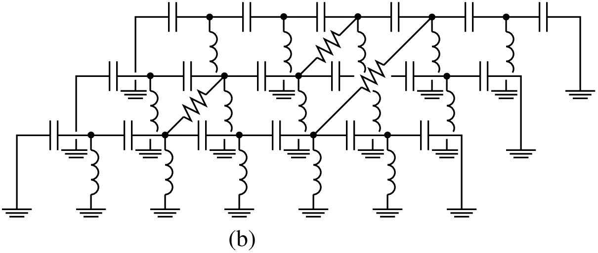
For instance, consider the individual electrical oscillator in Fig. 1, where unit (1H) inductors are connected by unit (1F) capacitors as shown. Let us form two separate arrays, each containing three identical replicas of this oscillator coupled via unit (1$\Omega$) resistors as in Fig. 2a and Fig. 2b, respectively. Although neither array look more connected than the other to the eye, there is a significant qualitative difference in their behaviors: starting from arbitrary initial conditions the oscillators in Fig. 2a always synchronize in the steady state, whereas those in Fig. 2b do not tend to oscillate in unison. This failure to synchronize can be traced back to the lack of connectivity of a certain graph.

Implicit in the above example is the importance of the role connectivity plays in network controllability. In fact, if the resistors in Fig. 2b are replaced by current sources (as our control inputs) the new array cannot be steered toward synchronization. The reason, not surprisingly, is the disconnectivity of the graph that was behind the failure of synchronization in the old array. To see the relation between connectivity and controllability explicitly, let us visit a simpler example where the graph is not hidden. Consider three identical water tanks (integrators) connected via water pumps as shown in Fig. 3.

Letting $x_{i}$ denote the water volume (${\rm m}^{3}$) contained in the $i$th tank and $u_{\sigma}$ the flow rate (${\rm m}^{3}/{\rm h}$) through the $\sigma$th pump we can write the dynamics as

$\displaystyle\left[\begin{array}[]{c}{\dot{x}}_{1}\\ {\dot{x}}_{2}\\ {\dot{x}}_{3}\end{array}\right]=\underbrace{\left[\begin{array}[]{rr}1&0\\ -1&1\\ 0&-1\end{array}\right]}_{\displaystyle B}\left[\begin{array}[]{c}u_{1}\\ u_{2}\end{array}\right]\,.$

The pleasant (zero column sum) structure of the matrix $B$ is shared by the incidence matrix representing the graph $\Gamma$ in Fig. 4. Observe that $\Gamma$ is (weakly) connected¹¹ 1 In this paper by connected we mean weakly connected. yet not strongly connected. This has two apparent implications. First, because the graph $\Gamma$ is connected the array is (relatively) controllable by which we mean that the relative states $x_{i}-x_{j}$ can be adjusted arbitrarily. That is, with bidirectional pumps the relative water levels can be simultaneously steered to any desired values regardless of the initial distribution. Second, because the graph $\Gamma$ is not strongly connected the array is not positively controllable. This translates to that with unidirectional pumps ($u_{\sigma}\geq 0$) the water levels cannot in general be equalized. At least three pumps are needed for that since at least three edges are needed for a 3-node graph to be strongly connected.

The water tanks example clearly illustrates the link between network controllability and graph connectivity. Meanwhile, as the oscillator array example indicates, the graphs whose connectivity determines controllability may not be apparent and therefore revealing them may require some effort. This paper is a report on such effort. Our setup is an array of linear time-invariant (LTI) systems driven by relative actuators. Specifically, the $i$th individual system’s ($n$th order) dynamics reads ${\dot{x}}_{i}=Ax_{i}+\sum_{\sigma}B_{i\sigma}u_{\sigma}$ with $\sum_{i}B_{i\sigma}=0$. For this setup we study, from the connectivity point of view, four problems: controllability, positive controllability, pairwise controllability, and positive pairwise controllability.

Controllability. The literature on network controllability has so far concentrated on a somewhat different problem concerning a different setup than ours given above. The generally adopted node dynamics are first order and there is coupling between nodes even when the inputs are zero. In addition, there is no relative actuation constraint. Namely, ${\dot{x}}_{i}=\sum_{j}a_{ij}x_{j}+\sum_{\sigma}b_{i\sigma}u_{\sigma}$ where $x_{i}\in{\mathbb{R}}$. Since the inputs are not relative, complete controllability is possible and that is what has been thoroughly investigated. Generally speaking, the problem that has received much attention concerns with the question of how to achieve controllability with as few inputs (or driver nodes) as possible; see, for instance, [12, 8, 19, 10]. In this particular direction a wealth of results has accumulated, e.g., [9, 2, 11, 16, 15], starting possibly with Lin’s work [6] on structural controllability. While these work dwell upon the “how?” for networks with first order node dynamics, we focus (in Section 4) on the simpler “yes/no?” for higher order dynamics. Namely, for an array with $q$ systems (nodes) and $p$ (relative) inputs, represented by the pair $[A,\,(B_{i\sigma})_{i,\sigma=1}^{q,p}]$ we present a necessary and sufficient condition for controllability²² 2 As mentioned earlier, when we use the word controllable to indicate an array we mean that all relative states $x_{i}-x_{j}$ (as opposed to actual states $x_{i}$) can be controlled. Since the actuation is relative in our setup, this is the most that can be achieved in terms of controllability. For instance, the total amount of water in the tanks in Fig. 3 is constant and therefore independent of the control inputs driving the array. from the graph connectivity point of view. The result is based on tools from classical control theory. The presented connectivity condition can indeed be seen as a certain reformulation of Popov-Belevitch-Hautus (PBH) test exploiting the special structure of our setup.

Positive controllability. ³³ 3 The term “positive controllability” seems to have been coined by Yoshida and his coauthors in the paper [17]. One of the earliest things we learn in life is how to steer a particular system (our body) with one-way actuators, for our muscles function that way. That is, a muscle can only pull or contract, but cannot (actively) push or extend. Another instance from biology of a one-way actuator is insulin, a key hormone in regulating the sugar level in blood. Insulin cannot undo what it does therefore pancreas employs another one-way agent, glucagon, to achieve proper regulation. Examples are not scarce outside biology; see, for instance, [4] and references therein. The earliest work on controllability of LTI systems with positive controls (one-way actuators) is [14]. Later Brammer provides a general eigenvector test [1] which arguably is the most effective tool we have today on positive controllability of continuous-time LTI systems. Certain refinements/reformulations of Brammer’s test are reported in [5, 18]. Among the very few works on positive controllability of networks is [7], where the authors study first order node dynamics. Here, for arrays with $n$th order node dynamics, we provide in Section 5 a necessary and sufficient strong connectivity condition for the positive controllability of an array. Just as our connectivity condition for controllability can be seen as a reformulation of PBH test, our strong connectivity condition for positive controllability is a natural extension of the refinements [18, 7] of Brammer’s eigenvector test.

Pairwise controllability. For an uncontrollable array, while it is not possible to steer all relative states, it is of interest to determine the subarrays of states that can be controlled relatively. The problem, at least for primitive arrays, is closely related to determining the connected components of an unconnected graph, which can be studied by means of paths connecting pairs of nodes. This motivates us to analyze (from connectivity point of view) the so called pairwise controllability, roughly described as follows. For a given pair $(k,\,\ell)$ of indices, an array is $(k,\,\ell)$-controllable when the difference $x_{k}-x_{\ell}$ can be arbitrarily adjusted. (The actual definition is subtler; see Def. 2.) The outcome of our analysis is presented in Section 6, where we provide necessary and sufficient connectivity conditions for $(k,\,\ell)$-controllability. From the geometric point of view what is done is in effect checking whether a certain subspace (corresponding to $(k,\,\ell)$-controllability of the array) is contained in the overall controllable subspace.

Positive pairwise controllability. Last in our sequence of problems is the characterization of pairwise controllability of an array with positive controls. The off-the-shelf tools (such as controllability matrix, PBH test, Brammer’s test) we use for the previous problems turn out not to be of much help here. Hence the analysis is of slightly different spirit and lengthier than before. However the end results (presented in Section 7) are of the same nature. In particular, positive pairwise controllability is interpreted in terms of strong connectivity of a pair of graph nodes.

To summarize, the contribution of this paper is intended to be in showing that the well-known close relation between controllability and connectivity for arrays with first order node dynamics naturally continue to exist for a class of arrays with higher order node dynamics. To this end, we study the above mentioned four facets of (relative) controllability. In particular, we establish connectivity characterizations of (pairwise) controllability as well as strong connectivity characterizations of positive (pairwise) controllability. With the possible exception of the contents of Section 7, the analysis methods employed in our work are not new; we borrow a great deal from the classical control theory toolbox. However, what we believe is fresh here is the perspective through which we tackle the problems at hand.

A pair $[A,\,(B_{i\sigma})_{i,\sigma=1}^{q,p}]$ is meant to represent an array of $q\geq 2$ LTI systems

$\displaystyle{\dot{x}}_{i}$

$\displaystyle=$

$\displaystyle Ax_{i}+\sum_{\sigma=1}^{p}B_{i\sigma}u_{\sigma}\,,\qquad i=1,\,2,\,\ldots,\,q$

(10)

where $x_{i}\in{\mathbb{R}}^{n}$ is the state of the $i$th system with $A\in{\mathbb{R}}^{n\times n}$. The $\sigma$th (scalar) input is denoted by $u_{\sigma}\in{\mathbb{R}}$. The input matrices $B_{i\sigma}\in{\mathbb{R}}^{n\times 1}$ are assumed to satisfy

$\displaystyle\sum_{i=1}^{q}B_{i\sigma}=0\,,\qquad\sigma=1,\,2,\,\ldots,\,p\,.$

(11)

The constraint (11) means that the actuation is relative. Hence the average of the states $x_{\rm av}=q^{-1}\sum x_{i}$ evolves independently of the inputs driving the array, i.e., we have ${\dot{x}}_{\rm av}=Ax_{\rm av}$. The shorthand notation $(B_{::})$ represents the ordered collection $(B_{i\sigma})_{i,\sigma=1}^{q,p}$. Given some $d\times n$ matrix $M$, we write $(MB_{::})$ to mean the collection $(\tilde{B}_{i\sigma})_{i,\sigma=1}^{q,p}$ with $\tilde{B}_{i\sigma}=MB_{i\sigma}$. For an index set $\mathcal{I}=\{\sigma_{1},\,\sigma_{2},\,\ldots,\,\sigma_{r}\}\subset\{1,\,2,\,\ldots,\,p\}$ the subcollection $(B_{i\sigma})_{i=1,\sigma\in\mathcal{I}}^{q}$ is denoted by $(B_{:\sigma})_{\sigma\in\mathcal{I}}$. The corresponding incidence matrix is constructed as

$\displaystyle{\rm inc}\,(B_{:\sigma})_{\sigma\in\mathcal{I}}=\left[\begin{array}[]{cccc}B_{1\sigma_{1}}&B_{1\sigma_{2}}&\cdots&B_{1\sigma_{r}}\\ B_{2\sigma_{1}}&B_{2\sigma_{2}}&\cdots&B_{2\sigma_{r}}\\ \vdots&\vdots&\ddots&\vdots\\ B_{q\sigma_{1}}&B_{q\sigma_{2}}&\cdots&B_{q\sigma_{r}}\end{array}\right]\,.$

Our goal in this paper is to interpret the above definitions in terms of connectivity properties of certain graphs related to the array (10). In particular, we characterize (positive) controllability and (positive) $(k,\,\ell)$-controllability in terms of (strong) connectivity and (strong) $(k,\,\ell)$-connectivity, respectively. Since our analysis heavily depends on graphs it is worthwhile to recall the relevant basics of graph theory. This we do next.

The next few definitions are borrowed from [3]. The convex cone that is positively spanned by the vectors $g_{1},\,g_{2},\,\ldots,\,g_{p}\in{\mathbb{R}}^{q}$ is defined as

$\displaystyle{\rm cone}\,\{g_{1},\,g_{2},\,\ldots,\,g_{p}\}=\left\{\zeta:\zeta=\sum_{\sigma=1}^{p}\alpha_{\sigma}g_{\sigma},\,\alpha_{\sigma}\in{\mathbb{R}}_{\geq 0}\right\}\,.$

In other words, ${\rm cone}\,\{g_{1},\,g_{2},\,\ldots,\,g_{p}\}$ is the set of all positive combinations of $g_{1},\,g_{2},\,\ldots,\,g_{p}$. For $\alpha\in{\mathbb{R}}^{p}$ we write $\alpha\geq 0$ to mean $\alpha$ has no negative entry. Likewise, $\alpha\leq 0$ means $-\alpha\geq 0$. The convex cone spanned by the columns of a matrix $G$ is denoted by ${\rm cone}\,G$. That is, ${\rm cone}\,G=\{\zeta:\zeta=G\alpha,\,\alpha\geq 0\}$. The range and null spaces of $G$ are denoted by ${\rm range}\,G$ and ${\rm null}\,G$, respectively. The conjugate transpose of $G$ is denoted by $G^{*}$. (If $G$ is real then $G^{*}$ is simply the transpose of $G$.) The synchronization subspace is defined as $\mathcal{S}_{n}={\rm range}\,[{\mathbf{1}}_{q}\otimes I_{n}]$, where ${\mathbf{1}}_{q}$ is the $q$-vector of all ones and $I_{n}$ is the $n\times n$ identity matrix. $\mathcal{S}_{n}^{\perp}$ denotes the orthogonal complement of $\mathcal{S}_{n}$. We say $G$ belongs to class-$\mathcal{G}_{n}$ ($G\in\mathcal{G}_{n}$) if ${\rm range}\,G\subset\mathcal{S}_{n}^{\perp}$. We let $e_{i}$ be the unit $q$-vector with $i$th entry one and the remaining entries zero.

A (directed) graph $\Gamma=(\mathcal{V},\,\mathcal{E},\,g)$ has a set of vertices (or nodes) $\mathcal{V}=\{v_{1},\,v_{2},\,\ldots,\,v_{q}\}$, a set of edges (or arcs) $\mathcal{E}=\{a_{1},\,a_{2},\,\ldots,\,a_{p}\}$, and a function $g:\mathcal{E}\to\mathcal{V}\times\mathcal{V}$ that maps each edge to an ordered pair $g(a_{\sigma})=(v_{i},\,v_{j})$ for some $i\neq j$. We allow parallel edges, i.e., $g$ need not be injective. By slight abuse of notation we sometimes call $(v_{i},\,v_{j})$ an edge and write $(v_{i},\,v_{j})\in\mathcal{E}$ when some $a_{\sigma}\in\mathcal{E}$ exists satisfying $g(a_{\sigma})=(v_{i},\,v_{j})$. Also, we write $-(v_{i},\,v_{j})$ to mean $(v_{j},\,v_{i})$. A directed path from $v_{k}$ to $v_{\ell}$ ($k\neq\ell$) is a sequence of pairs $((v_{i_{1}},\,v_{i_{2}}),\,(v_{i_{2}},\,v_{i_{3}}),\,\ldots,\,(v_{i_{r}},\,v_{i_{r+1}}))$ satisfying $i_{1}=k$, $i_{r+1}=\ell$, and $(v_{i_{j}},\,v_{i_{j+1}})\in\mathcal{E}$ for all $j=1,\,2,\,\ldots,\,r$. An undirected path between $v_{k}$ and $v_{\ell}$ ($k\neq\ell$) is a sequence of pairs $((v_{i_{1}},\,v_{i_{2}}),\,(v_{i_{2}},\,v_{i_{3}}),\,\ldots,\,(v_{i_{r}},\,v_{i_{r+1}}))$ satisfying $i_{1}=k$, $i_{r+1}=\ell$, and for each $j=1,\,2,\,\ldots,\,r$ either $(v_{i_{j}},\,v_{i_{j+1}})$ or $(v_{i_{j+1}},\,v_{i_{j}})$ belongs to $\mathcal{E}$. We adopt the convention that there is a (un)directed path from each vertex to itself despite that we allow no loop edges $(v_{i},\,v_{i})$. For $k\neq\ell$ the graph $\Gamma$ is said to be strongly $(k,\,\ell)$-connected if there exist two directed paths, one from $v_{k}$ to $v_{\ell}$, the other from $v_{\ell}$ to $v_{k}$. It is said to be $(k,\,\ell)$-connected if there exists an undirected path between $v_{k}$ and $v_{\ell}$. It is said to be (strongly) connected if it is (strongly) $(k,\,\ell)$-connected for all $(k,\,\ell)$. The incidence matrix $[g_{i\sigma}]=G\in{\mathbb{R}}^{q\times p}$ of the graph $\Gamma$ is such that the edge $a_{\sigma}$ with $g(a_{\sigma})=(v_{i},\,v_{j})$ is represented by the $\sigma$th column of $G$ in the following way: $g_{i\sigma}=1$, $g_{j\sigma}=-1$, and the remaining entries of the column are zero. I.e., $g(a_{\sigma})=(v_{i},\,v_{j})$ implies $\sigma$th column of $G$ equals $e_{i}-e_{j}$. Note that $G\in\mathcal{G}_{1}$ since ${\mathbf{1}}_{q}^{*}G=0$. We now make the following simple observations.

Let us establish the other direction by contradiction. Suppose there does not exist a directed path from $v_{k}$ to $v_{\ell}$ while ${\rm cone}\,G\supset{\rm range}\,[e_{k}-e_{\ell}]$. Let $\mathcal{V}_{k}\subset\mathcal{V}$ be the set of all vertices to which there is a directed path from $v_{k}$. Similarly, let $\mathcal{V}_{\ell}\subset\mathcal{V}$ be the set of all vertices from which there is a directed path to $v_{\ell}$. (Note that $v_{k}\in\mathcal{V}_{k}$ and $v_{\ell}\in\mathcal{V}_{\ell}$.) Since no directed path exists from $v_{k}$ to $v_{\ell}$, the sets $\mathcal{V}_{k}$ and $\mathcal{V}_{\ell}$ are disjoint. Now define the edge sets $\mathcal{E}_{k}=\{(v_{i},\,v_{j})\in\mathcal{E}:v_{i},\,v_{j}\in\mathcal{V}_{k}\}$ and $\mathcal{E}_{\ell}=\{(v_{i},\,v_{j})\in\mathcal{E}:v_{i},\,v_{j}\in\mathcal{V}_{\ell}\}$, which, too, are disjoint. Let $G_{k}$ and $G_{\ell}$ be the incidence matrices of the subgraphs $\Gamma_{k}=(\mathcal{V}_{k},\,\mathcal{E}_{k},\,g)$ and $\Gamma_{\ell}=(\mathcal{V}_{\ell},\,\mathcal{E}_{\ell},\,g)$, respectively. Since the vertices and edges can be relabeled, we can assume, without loss of generality, $G$ has the following block structure.

$\displaystyle G=\left[\begin{array}[]{c}\!\!\!\!\begin{array}[]{c}G_{k}\\ 0\\ 0\end{array}\vline\begin{array}[]{l}M_{-}\\ M_{*}\\ M_{+}\end{array}\vline\begin{array}[]{c}0\\ 0\\ G_{\ell}\end{array}\end{array}\right]=\left[\begin{array}[]{clc}G_{k}&M_{-}&0\\ \hline\cr\\ 0&M_{*}&0\\ \hline\cr\\ 0&M_{+}&G_{\ell}\end{array}\right]$

For the ease of discussion $G$ is partitioned in various ways as shown above. Observe that the entries of the matrix $M_{-}$ (if exists) are either $0$ or $-1$. To see that suppose otherwise, i.e., $M_{-}$ has an entry $g_{i\sigma}=1$. Let $j$ be such that $g_{j\sigma}=-1$. Since $g_{i\sigma}$ belongs to the center column partition, the edge $a_{\sigma}$ (satisfying $g(a_{\sigma})=(v_{i},\,v_{j})$) can belong neither to $\mathcal{E}_{k}$ nor to $\mathcal{E}_{\ell}$. Moreover, $v_{i}\in\mathcal{V}_{k}$ because $g_{i\sigma}$ belongs to the upper row partition. By definition, $v_{i}\in\mathcal{V}_{k}$ implies there is a directed path from $v_{k}$ to $v_{i}$. The existence of the edge $(v_{i},\,v_{j})$ implies that this path can be extended to $v_{j}$. Consequently $v_{j}\in\mathcal{V}_{k}$. Since both vertices $v_{i},\,v_{j}$ belong to $\mathcal{V}_{k}$ we have to have $a_{\sigma}\in\mathcal{E}_{k}$, but this we already ruled out. Therefore $M_{-}$ can have only nonpositive entries.

Since ${\rm cone}\,G\supset{\rm range}\,[e_{k}-e_{\ell}]$ we can find a $p$-vector $\alpha\geq 0$ satisfying $G\alpha=e_{k}-e_{\ell}$. Let $q_{k}$ be the number of vertices in $\mathcal{V}_{k}$ and $q_{\ell}$ the number of vertices in $\mathcal{V}_{\ell}$. We can write

$\displaystyle G\alpha=\left[\begin{array}[]{clc}G_{k}&M_{-}&0\\ \hline\cr\\ 0&M_{*}&0\\ \hline\cr\\ 0&M_{+}&G_{\ell}\end{array}\right]\alpha=\left[\begin{array}[]{c}f_{+}\\ \hline\cr\\ f_{0}\\ \hline\cr\\ f_{-}\end{array}\right]=e_{k}-e_{\ell}$

where $f_{+}\in{\mathbb{R}}^{q_{k}}$ and $f_{-}\in{\mathbb{R}}^{q_{\ell}}$. Since $k\leq q_{k}$ and $\ell\geq q-q_{\ell}+1>q_{k}$ the vector $f_{+}=[G_{k}\ M_{-}\ 0]\alpha$ contains exactly one $+1$ entry while its other entries are zero. (Likewise, $f_{-}$ contains exactly one $-1$ entry while its other entries are zero and $f_{0}$ (if exists) is a vector of zeros.) In particular, ${\bf 1}_{q_{k}}^{*}f_{+}=1$. Now define $\beta=[G_{k}\ M_{-}\ 0]^{*}{\bf 1}_{q_{k}}$. Using $G_{k}^{*}{\bf 1}_{q_{k}}=0$ (because $G_{k}$ is an incidence matrix) and the fact that $M_{-}$ has no positive entry we can write $\beta=[G_{k}\ M_{-}\ 0]^{*}{\bf 1}_{q_{k}}=[0\ M_{-}\ 0]^{*}{\bf 1}_{q_{k}}\leq 0$. Combining $\beta\leq 0$ with $\alpha\geq 0$ yields $\beta^{*}\alpha\leq 0$. However this results in the following contradiction

$\displaystyle 1={\bf 1}_{q_{k}}^{*}f_{+}={\bf 1}_{q_{k}}^{*}[G_{k}\ M_{-}\ 0]\alpha=\beta^{*}\alpha\leq 0\,.$

2. Given $\Gamma=(\mathcal{V},\,\mathcal{E},\,g)$ with $\mathcal{V}=\{v_{1},\,v_{2},\,\ldots,\,v_{q}\}$ and $\mathcal{E}=\{a_{1},\,a_{2},\,\ldots,\,a_{p}\}$, define the mapping $g_{\rm a}:\mathcal{E}_{\rm a}\to\mathcal{V}\times\mathcal{V}$ for the augmented edge set $\mathcal{E}_{\rm a}=\{a_{1},\,a_{2},\,\ldots,\,a_{2p}\}$ as follows.

$\displaystyle g_{\rm a}(a_{\sigma})=\left\{\begin{array}[]{rcl}g(a_{\sigma})&\mbox{for}&\sigma=1,\,2,\,\ldots,\,p\\ -g(a_{\sigma})&\mbox{for}&\sigma=p+1,\,p+2,\,\ldots,\,2p\,.\end{array}\right.$

Let $\Gamma_{\rm a}=(\mathcal{V},\,\mathcal{E}_{\rm a},\,g_{\rm a})$. It is not hard to see that $\Gamma$ is $(k,\,\ell)$-connected if and only if $\Gamma_{\rm a}$ is strongly $(k,\,\ell)$-connected. Moreover, the incidence matrix of $\Gamma_{\rm a}$ reads $G_{\rm a}=[G\ -G]$. Therefore ${\rm cone}\,G_{\rm a}={\rm range}\,G$. Using the first statement of the proposition we can now write

	$\Gamma$ $(k,\,\ell)$-connected	$\displaystyle\Longleftrightarrow$	$\Gamma_{\rm a}$ strongly $(k,\,\ell)$-connected
		$\displaystyle\Longleftrightarrow$	$\displaystyle{\rm cone}\,G_{\rm a}\supset{\rm range}\,[e_{k}-e_{\ell}]$
		$\displaystyle\Longleftrightarrow$	$\displaystyle{\rm range}\,G\supset{\rm range}\,[e_{k}-e_{\ell}]\,.$

3. If $\Gamma$ is strongly connected, then, by definition, $\Gamma$ is strongly $(k,\,\ell)$-connected for all pairs $(k,\,\ell)$. The first statement of the proposition then allows us to write

$\displaystyle{\rm cone}\,G\supset\sum_{k,\ell}\,{\rm range}\,[e_{k}-e_{\ell}]=\mathcal{S}_{1}^{\perp}\,.$

If $\Gamma$ is not strongly connected, then there exists a pair $(k,\,\ell)$ for which ${\rm cone}\,G\not\supset{\rm range}\,[e_{k}-e_{\ell}]$. Since $\mathcal{S}_{1}^{\perp}\supset{\rm range}\,[e_{k}-e_{\ell}]$ we have to have ${\rm cone}\,G\not\supset\mathcal{S}_{1}^{\perp}$.

4. The result follows from the second statement. The demonstration is similar to that of the third statement.   $\blacksquare$

Proposition 1 motivates us for the following generalization.

A brief digression is in order here. Definition 3 intends to extend connectivity, a central notion for graphs, to class-$\mathcal{G}_{n}$ matrices, which may be taken to represent (or be) generalized graphs. In this representation each column of $G\in\mathcal{G}_{n}$ may be treated as an edge. Then a path between $k$th and $\ell$th vertices may be said to exist if for each $\eta\in{\mathbb{R}}^{n}$ we can find some edges (columns) $g_{\sigma}$ and some weights $\alpha_{\sigma}$ that take us from vertex $k$ to vertex $\ell$ by satisfying $e_{k}\otimes\eta+\alpha_{1}g_{1}+\alpha_{2}g_{2}+\cdots+\alpha_{r}g_{r}=e_{\ell}\otimes\eta$. (For a directed path we would require the weights to be positive.) Depicting the endpoints $e_{k}\otimes\eta$ and $e_{\ell}\otimes\eta$ as dots (in space they belong to) and the vectors $\alpha_{\sigma}g_{\sigma}$ as successive line segments connecting the two dots, a geometric interpretation can be obtained. Hence, although it would be difficult (provided it is possible/meaningful) to draw a generalized graph, the notion of connectivity seems to maintain to some degree its visual feature.

Definition 3 has an interesting claim on hypergraphs,⁴⁴ 4 A hypergraph is such that each edge is allowed to be incident to more than two vertices. which can be observed on a simple instance. Consider the array (1) of water tanks under the constraint $u_{2}=2u_{1}$ which arises, say, because the voltages driving the water pumps are not independent. Then the dynamics reads $[{\dot{x}}_{1}\ {\dot{x}}_{2}\ {\dot{x}}_{3}]^{*}=[1\ \ 1\ -2]^{*}u_{1}$. Let now $G=[1\ \ 1\ -2]^{*}\in\mathcal{G}_{1}$ represent the incidence matrix of a 3-vertex graph; call this graph $\Gamma$. Since $G$ has a single column, $\Gamma$ has a single edge. This edge is incident to all the vertices, for the corresponding column has no zero entries. Therefore $\Gamma$ is a 3-vertex hypergraph with a single (hyper)edge that is incident to all three vertices. According to the classical definition of connectivity for hypergraphs, $\Gamma$ is connected because any two vertices are adjacent to one another through the only edge. According to Definition 3 however, $G$ (therefore $\Gamma$) is not connected. In fact, no two vertices are connected since ${\rm range}\,G\not\supset{\rm range}\,[e_{k}-e_{\ell}]$ for all pairs $(k,\,\ell)$. To support Definition 3 against this discrepancy let us first obtain the Laplacian matrix $L$ of $\Gamma$ from the incidence matrix $G$ as

$\displaystyle L=GG^{*}=\left[\begin{array}[]{rrr}1&1&-2\\ 1&1&-2\\ -2&-2&4\end{array}\right]\,.$

Then, treating $L$ as the node admittance matrix of a resistive network, we obtain the conductances $\gamma_{ij}$ between the nodes $i$ and $j$ through

$\displaystyle\left[\begin{array}[]{ccc}\gamma_{12}+\gamma_{31}&-\gamma_{12}&-\gamma_{31}\\ -\gamma_{12}&\gamma_{23}+\gamma_{12}&-\gamma_{23}\\ -\gamma_{31}&-\gamma_{23}&\gamma_{31}+\gamma_{23}\end{array}\right]=L$

as $\gamma_{12}=-1\mho$, $\gamma_{23}=2\mho$, and $\gamma_{31}=2\mho$. These values yield the simple delta network in Fig. 5.

Now, the connectivity of this network can be determined via the circuit theory tool effective conductance. Namely, the vertices $k$ and $\ell$ of the graph $\Gamma$ is connected if the effective conductance between the nodes $k$ and $\ell$ of the corresponding resistive network in Fig. 5 is positive. A quick calculation shows that the effective conductance for any pair of nodes is zero for this network. Hence no two vertices of $\Gamma$ is connected, just as Definition 3 predicates.

In the remainder of the paper we attempt to interpret different controllability aspects of the array (10) in terms of (strong) connectivity properties of certain class-$\mathcal{G}_{n}$ matrices.

Consider the array (10). By $\mu_{1},\,\mu_{2},\,\ldots,\,\mu_{m}$ we denote the distinct eigenvalues of $A^{*}$. Note that $m\leq n$ and these eigenvalues are shared by $A$. For each $\kappa\in\{1,\,2,\,\ldots,\,m\}$ we let $V_{\kappa}\in{\mathbb{C}}^{n\times d_{\kappa}}$ denote a full column rank matrix satisfying ${\rm range}\,V_{\kappa}={\rm null}\,[A^{*}-\mu_{\kappa}I_{n}]$. Therefore $d_{\kappa}$ is the geometric multiplicity of the eigenvalue $\mu_{\kappa}$. We let $V_{\kappa}\in{\mathbb{R}}^{n\times d_{\kappa}}$ when $\mu_{\kappa}\in{\mathbb{R}}$. Note that the columns of $V_{\kappa}$ are the linearly independent eigenvectors of $A^{*}$ corresponding to the eigenvalue $\mu_{\kappa}$. In particular, we have $A^{*}V_{\kappa}=\mu_{\kappa}V_{\kappa}$. For notational convenience we sometimes represent the array (10) as a single big system

$\displaystyle{\dot{}{\mathbf{x}}}={\mathbf{A}}{\mathbf{x}}+{\mathbf{B}}{\mathbf{u}}$

(19)

where ${\mathbf{x}}=[x_{1}^{*}\ x_{2}^{*}\ \cdots\ x_{q}^{*}]^{*}$ is the state and ${\mathbf{u}}=[u_{1}\ u_{2}\ \cdots\ u_{p}]^{*}$ is the input. Clearly, we have

$\displaystyle{\mathbf{A}}=[I_{q}\otimes A]$

while ${\mathbf{B}}\in{\mathbb{R}}^{(qn)\times p}$ has the structure

$\displaystyle{\mathbf{B}}={\rm inc}\,(B_{::})=\left[\begin{array}[]{cccc}B_{11}&B_{12}&\cdots&B_{1p}\\ B_{21}&B_{22}&\cdots&B_{2p}\\ \vdots&\vdots&\ddots&\vdots\\ B_{q1}&B_{q2}&\cdots&B_{qp}\end{array}\right]\,.$

Note that ${\mathbf{B}}\in\mathcal{G}_{n}$ due to (11) and ${\rm inc}\,(V_{\kappa}^{*}B_{::})=[I_{q}\otimes V_{\kappa}^{*}]{\mathbf{B}}$. The controllability matrix associated to the pair $[{\mathbf{A}},\,{\mathbf{B}}]$ reads $[{\mathbf{B}}\ {\mathbf{A}}{\mathbf{B}}\ \cdots\ {\mathbf{A}}^{qn-1}{\mathbf{B}}]$. However, being equal to $[I_{q}\otimes A]$, the matrix ${\mathbf{A}}$ satisfies the characteristic equation of $A$ (which is of order $n$) and therefore the controllability index for the pair $[{\mathbf{A}},\,{\mathbf{B}}]$ is at most $n$. Hence we can treat

$\displaystyle{\mathbf{W}}=[{\mathbf{B}}\ {\mathbf{A}}{\mathbf{B}}\ \cdots\ {\mathbf{A}}^{n-1}{\mathbf{B}}]$

as the controllability matrix. Indeed, ${\rm range}\,{\mathbf{W}}$ is the controllable subspace for the pair $[{\mathbf{A}},\,{\mathbf{B}}]$. Observe ${\mathbf{W}}\in\mathcal{G}_{n}$. Recall that the vector ${\bf 1}_{q}$ spans the synchronization subspace $\mathcal{S}_{1}$. Let $S$ denote its normalized version, i.e., $S={\bf 1}_{q}/\sqrt{q}$ and hence $S^{*}S=1$. Also, let $D\in{\mathbb{R}}^{q\times(q-1)}$ be some matrix whose columns make an orthonormal basis for $\mathcal{S}_{1}^{\perp}$, sometimes called the disagreement subspace. Note that $D^{*}D=I_{q-1}$ and the columns of the matrix $[D\ S]$ make an orthonormal basis for ${\mathbb{R}}^{n}$. The following identities are easy to show and find frequent use in the sequel.

1. (i)

   $DD^{*}+SS^{*}=I_{q}$.

2. (ii)

   ${\rm range}\,[D\otimes I_{n}]=\mathcal{S}_{n}^{\perp}$.

3. (iii)

   ${\rm null}\,[D^{*}\otimes I_{n}]=\mathcal{S}_{n}$.

4. (iv)

   $[S^{*}\otimes I_{n}]{\mathbf{B}}=0$.

The distance of ${\mathbf{x}}$ to $\mathcal{S}_{n}$ we denote by $\|{\mathbf{x}}\|_{\mathcal{S}_{n}}=\left\|[D^{*}\otimes I_{n}]{\mathbf{x}}\right\|$. Finally, we define the reduced parameters

	$\displaystyle{\mathbf{A}}_{\rm r}$	$\displaystyle=$	$\displaystyle[I_{q-1}\otimes A]$
	$\displaystyle{\mathbf{B}}_{\rm r}$	$\displaystyle=$	$\displaystyle[D^{*}\otimes I_{n}]{\mathbf{B}}$
	$\displaystyle{\mathbf{W}}_{\rm r}$	$\displaystyle=$	$\displaystyle[{\mathbf{B}}_{\rm r}\ {\mathbf{A}}_{\rm r}{\mathbf{B}}_{\rm r}\ \cdots\ {\mathbf{A}}_{\rm r}^{n-1}{\mathbf{B}}_{\rm r}]\,.$

The controllability index for the pair $[{\mathbf{A}}_{\rm r},\,{\mathbf{B}}_{\rm r}]$ is at most $n$. Hence ${\rm range}\,{\mathbf{W}}_{\rm r}$ equals the controllable subspace associated to the pair $[{\mathbf{A}}_{\rm r},\,{\mathbf{B}}_{\rm r}]$.

3$\implies$2. Suppose $[{\mathbf{A}}_{\rm r},\,{\mathbf{B}}_{\rm r}]$ is controllable. Observe that we can write for all $k\in\{0,\,1,\,\ldots,\,n-1\}$

	$\displaystyle{\mathbf{A}}_{\rm r}^{k}{\mathbf{B}}_{\rm r}$	$\displaystyle=$	$\displaystyle[I_{q-1}\otimes A]^{k}[D^{*}\otimes I_{n}]{\mathbf{B}}$
		$\displaystyle=$	$\displaystyle[I_{q-1}\otimes A^{k}][D^{*}\otimes I_{n}]{\mathbf{B}}$
		$\displaystyle=$	$\displaystyle[D^{*}\otimes I_{n}][I_{q}\otimes A^{k}]{\mathbf{B}}$
		$\displaystyle=$	$\displaystyle[D^{*}\otimes I_{n}][I_{q}\otimes A]^{k}{\mathbf{B}}$
		$\displaystyle=$	$\displaystyle[D^{*}\otimes I_{n}]{\mathbf{A}}^{k}{\mathbf{B}}$

yielding ${\mathbf{W}}_{\rm r}=[D^{*}\otimes I_{n}]{\mathbf{W}}$. Similarly, using $[S^{*}\otimes I_{n}]{\mathbf{B}}=0$ we can write

	$\displaystyle[S^{*}\otimes I_{n}]{\mathbf{A}}^{k}{\mathbf{B}}$	$\displaystyle=$	$\displaystyle[S^{*}\otimes I_{n}][I_{q}\otimes A^{k}]{\mathbf{B}}$
		$\displaystyle=$	$\displaystyle A^{k}[S^{*}\otimes I_{n}]{\mathbf{B}}$
		$\displaystyle=$	$\displaystyle 0$

yielding $[S^{*}\otimes I_{n}]{\mathbf{W}}=0$. Since $[{\mathbf{A}}_{\rm r},\,{\mathbf{B}}_{\rm r}]$ is controllable, ${\mathbf{W}}_{\rm r}$ is full column rank, which allows us to write ${\rm range}\,[D\otimes I_{n}]{\mathbf{W}}_{\rm r}={\rm range}\,[D\otimes I_{n}]$. Let us now gather our recent findings and obtain

	$\displaystyle{\rm range}\,{\mathbf{W}}$	$\displaystyle=$	$\displaystyle{\rm range}\,[(DD^{*}+SS^{*})\otimes I_{n}]{\mathbf{W}}$
		$\displaystyle=$	$\displaystyle{\rm range}\,\left([D\otimes I_{n}][D^{*}\otimes I_{n}]{\mathbf{W}}+[S\otimes I_{n}][S^{*}\otimes I_{n}]{\mathbf{W}}\right)$
		$\displaystyle=$	$\displaystyle{\rm range}\,[D\otimes I_{n}]{\mathbf{W}}_{\rm r}$
		$\displaystyle=$	$\displaystyle{\rm range}\,[D\otimes I_{n}]$
		$\displaystyle=$	$\displaystyle\mathcal{S}_{n}^{\perp}\,.$

Therefore ${\rm range}\,{\mathbf{W}}\supset\mathcal{S}_{n}^{\perp}$.

2$\implies$1. Suppose ${\rm range}\,{\mathbf{W}}\supset\mathcal{S}_{n}^{\perp}$. Consider the system (19). Let ${\mathbf{x}}(0)$ be an arbitrary initial condition. Then let $\xi=[DD^{*}\otimes I_{n}]{\mathbf{x}}(0)$. Note that $\xi\in\mathcal{S}_{n}^{\perp}$. Therefore $\xi$ belongs to the controllable subspace ${\rm range}\,{\mathbf{W}}$ associated to the pair $[{\mathbf{A}},\,{\mathbf{B}}]$. Consequently we can find an input signal ${\mathbf{u}}:[0,\,\tau]\to{\mathbb{R}}^{p}$ with finite $\tau>0$ that satisfies

$\displaystyle e^{{\mathbf{A}}\tau}\xi+\int_{0}^{\tau}e^{{\mathbf{A}}(\tau-t)}{\mathbf{B}}{\mathbf{u}}(t)dt=0\,.$

Now using this control signal and the identity $D^{*}S=0$ we can write

	$\displaystyle[D^{*}\otimes I_{n}]{\mathbf{x}}(\tau)$	$\displaystyle=$	$\displaystyle[D^{*}\otimes I_{n}]\left(e^{{\mathbf{A}}\tau}{\mathbf{x}}(0)+\int_{0}^{\tau}e^{{\mathbf{A}}(\tau-t)}{\mathbf{B}}{\mathbf{u}}(t)dt\right)$
		$\displaystyle=$	$\displaystyle[D^{*}\otimes I_{n}]\left([(DD^{*}+SS^{*})\otimes e^{A\tau}]{\mathbf{x}}(0)+\int_{0}^{\tau}e^{{\mathbf{A}}(\tau-t)}{\mathbf{B}}{\mathbf{u}}(t)dt\right)$
		$\displaystyle=$	$\displaystyle[D^{*}\otimes I_{n}]\left([DD^{*}\otimes e^{A\tau}]{\mathbf{x}}(0)+\int_{0}^{\tau}e^{{\mathbf{A}}(\tau-t)}{\mathbf{B}}{\mathbf{u}}(t)dt\right)+[D^{*}SS^{*}\otimes e^{A\tau}]{\mathbf{x}}(0)$
		$\displaystyle=$	$\displaystyle[D^{*}\otimes I_{n}]\left([I_{q}\otimes e^{A\tau}][DD^{*}\otimes I_{n}]{\mathbf{x}}(0)+\int_{0}^{\tau}e^{{\mathbf{A}}(\tau-t)}{\mathbf{B}}{\mathbf{u}}(t)dt\right)$
		$\displaystyle=$	$\displaystyle[D^{*}\otimes I_{n}]\left(e^{{\mathbf{A}}\tau}\xi+\int_{0}^{\tau}e^{{\mathbf{A}}(\tau-t)}{\mathbf{B}}{\mathbf{u}}(t)dt\right)$
		$\displaystyle=$	$\displaystyle 0\,.$

That is, $\|{\mathbf{x}}(\tau)\|_{\mathcal{S}_{n}}=0$. The array $[A,\,(B_{::})]$ then has to be controllable because ${\mathbf{x}}(0)$ was arbitrary.   $\blacksquare$

References

• [1] R.F. Brammer. Controllability in linear autonomous systems with positive controllers. SIAM Journal of Control, 10:339–353, 1972.
• [2] C. Commault and J.-M. Dion. Input addition and leader selection for the controllability of graph-based systems. Automatica, 49:3322–3328, 2013.
• [3] C. Davis. Theory of positive linear dependence. American Journal of Mathematics, 76:733–746, 1954.
• [4] J. Eden, Y. Tang, D. Lau, and D. Oetomo. On the positive output controllability of linear time invariant systems. Automatica, 71:202–209, 2016.
• [5] M. Hermann and R.J. Stern. Controllability of linear systems with positive controls: geometric considerations. Journal of Mathematical Analysis and Applications, 52:36–41, 1975.
• [6] C.-T. Lin. Structural controllability. IEEE Transactions on Automatic Control, 19:201–208, 1974.
• [7] G. Lindmark and C. Altafini. Positive controllability of large-scale networks. In Proc. of the European Control Conference, pages 819–824, 2016.
• [8] Y.-Y. Liu, J.-J. Slotine, and A.-L. Barabasi. Controllability of complex networks. Nature, 473:167–173, 2011.
• [9] G. Notarstefano and G. Parlangeli. Controllability and observability of grid graphs via reduction and symmetries. IEEE Transactions on Automatic Control, 58:1719–1731, 2013.
• [10] A. Olshevsky. Minimal controllability problems. IEEE Transactions on Control of Network Systems, 1:249–258, 2014.
• [11] S. Pequito, S. Kar, and A.-P. Aguiar. A framework for structural input/output and control configuration selection in large-scale systems. IEEE Transactions on Automatic Control, 61:303–318, 2016.
• [12] A. Rahmani, M. Ji, M. Mesbahi, and M. Egerstedt. Controllability of multi-agent systems from a graph-theoretic perspective. SIAM Journal on Control and Optimization, 48:162–186, 2009.
• [13] R.T. Rockafellar. Convex Analysis. Princeton University Press, 1970.
• [14] S.H. Saperstone and J.A. Yorke. Controllability of linear oscillatory systems using positive controls. SIAM Journal of Control, 9:253–262, 1971.
• [15] L.-Z. Wang, Y.-Z. Chen, W.-X. Wang, and Y.-C. Lai. Physical controllability of complex networks. Scientific Reports, 7:40198, 2017.
• [16] W.-X. Wang, X. Ni, Y.-C. Lai, and C. Grebogi. Optimizing controllability of complex networks by minimum structural perturbations. Physical Review E, 85:026115, 2012.
• [17] H. Yoshida, Y. Tanada, T. Tanaka, and K. Yunokuchi. Controllability of multiple input discrete-time linear systems with positive controls. Transactions of the Society of Instrument and Control Enginners, 30:243–252, 1994.
• [18] H. Yoshida and T. Tanaka. Positive controllability test for continuous-time linear systems. IEEE Transactions on Automatic Control, 52:1685–1689, 2007.
• [19] Z. Yuan, C. Zhao, Z. Di, W.-X. Wang, and Y.-C. Lai. Exact controllability of complex networks. Nature Communications, 4:2447, 2013.