Scalarization of neutron stars with realistic equations of state

In four dimensions, the generic action for STT (with a single scalar field) is given in the Jordan frame by [8, 11, 9]

where $G_{*}$ is the gravitational constant, $\tilde{\cal R}$ is the Ricci scalar with respect the metric ${\tilde{g}_{\mu\nu}}$, and $\Phi$ is the scalar field. The term $S_{m}$ denotes the contribution of additional matter fields to the action, which are parametrized into $\Psi_{m}$. Here we restrict to the case where the scalar field does not couple directly to these additional matter fields, implying that the weak equivalence principle is satisfied. The gravitational part of the action includes the functions $F(\Phi)$ and $Z(\Phi)$, and the potential function $U(\Phi)$. These functions are subject to physical restrictions, as it was shown in [32]

For the study of neutron stars in this theory it is convenient to change to the Einstein frame. This frame is related to the Jordan frame by a conformal transformation of the metric $g_{\mu\nu}=F(\Phi){\tilde{g}}_{\mu\nu}$, and a transformation of the scalar field [8, 11, 9]. After this transformation the action becomes

where ${\cal R}$ is the Ricci scalar with respect to the metric $g_{\mu\nu}$, and $\varphi$ is the scalar field, both being defined in the Einstein frame. In addition we have the following relations between the Jordan frame functions $F(\Phi)$ and $U(\Phi)$ and the Einstein frame functions $A(\varphi)$ and $V(\varphi)$

Here we restrict to the case with vanishing scalar potential $U(\Phi)=0=V(\varphi)$. In the following we will use $c=G_{*}=1$ units unless otherwise stated.

Variation of the action (2) with respect to the fields in the Einstein frame leads to the coupled set of field equations. The Einstein equations read

where ${\cal R}_{\mu\nu}$ is the Ricci tensor, and $T_{\mu\nu}$ is the stress-energy tensor of the matter content of the action (2). The scalar field equation is given by

where $T=T^{\mu}_{\mu}$, and $k(\varphi)=\frac{d\ln({A}(\varphi))}{d\varphi}$ is the logarithmic derivative of the coupling function $A(\varphi)$, which determines the strength of the coupling between the scalar field and the matter.

We model the neutron star as a perfect fluid in (slow) uniform rotation. Hence in the physical Jordan frame the stress energy momentum tensor ${\tilde{T}}_{\mu\nu}$ is given by

where $\tilde{\varepsilon}$, $\tilde{p}$ and $\tilde{u}$ denote the energy density, the pressure and the four-velocity in the Jordan frame, respectively. In the Jordan frame we also assume a barotropic equation of state, i.e., $\tilde{\varepsilon}=\tilde{\varepsilon}(\tilde{p})$. The nuclear matter quantities $\tilde{\varepsilon}$, $\tilde{p}$ and $\tilde{u}$ in the Jordan frame are related to those in the Einstein frame via the conformal factor $F(\Phi)$ and can be found in [8, 11, 9].

The coupling function $A(\varphi)$ is subject to constraints from observations, leaving however a large amount of freedom for its functional choice. In the simple case $k(\varphi)=\kappa$, with $\kappa$ some arbitrary constant, a parameterization of the Brans-Dicke theory is obtained [7] where $A=e^{\kappa\varphi}$. Here we consider a set of two coupling functions, $A_{1}(\varphi)$ and $A_{2}(\varphi)$. The coupling function $A_{1}(\varphi)$ has been investigated widely before (see e.g. [8, 11, 19, 22])

The coupling function $A_{2}(\varphi)$ has not yet been considered, and corresponds to

Both coupling functions have been parametrized such that they possess the same quadratic expansion coefficient. They differ only in higher order, where the fall-off of ${A}_{2}(\varphi)$ is slower. This is in contrast to the coupling function $A_{3}(\varphi)=\cos{(\sqrt{-\beta}\varphi)}$ employed in [10], which exhibits a faster fall-off. Note that all of these three couplings are invariant under the transformation $\varphi\to-\varphi$.

The strongest observational constraint on the possible values of the constant $\beta$ that should be taken into account comes from the binary pulsar PSR J1738+0333 [33], which requires

In order to describe slowly rotating neutron stars, we choose the following form of the metric in the Einstein frame

where the metric functions $f(r)$, $n(r)$ and $\omega(r)$ depend only on the radial coordinate $r$. We introduce $\xi$ as a perturbation theory parameter, that allows us to keep track of the slow rotation approximation, i.e., all expressions are to be considered up to $O(\xi^{2})$.

The inertial dragging $\omega(r)$ vanishes in the static case. In the slow rotation approximation the scalar field is not affected by the rotation, since $\varphi=\varphi(r)+O(\xi^{2})$, and hence it is only a function of the radial coordinate. The same applies to the energy density $\tilde{\varepsilon}=\tilde{\varepsilon}(r)+O(\xi^{2})$ and the pressure $\tilde{p}=\tilde{p}(r)+O(\xi^{2})$. The four velocity of the fluid in the slow rotation approximation is $\tilde{u}=u^{t}(\partial_{t}+\xi\Omega\partial_{\phi})$, where $\Omega$ is the angular velocity of the fluid.

With the metric ansatz Eq. (10) and the above definitions the Einstein field equations in the slow rotation approximation reduce to a system of Ordinary Differential Equations (ODEs) that has been presented before in the literature [10, 11, 12, 14, 15] .

Regularity of the configurations at the center of the star ($r=0$) imposes a particular expansion in terms of the radial coordinate $r$, which can be found in [16].

The surface of the star is defined as the surface of constant radius $r=R$, where the pressure vanishes, $\tilde{p}|_{R}=0$. The exterior of the star is then given by $r>R$. Here the energy density and the pressure vanish: $\tilde{p}|_{r>R}=\tilde{\varepsilon}|_{r>R}=0$. However, the scalar field does not vanish outside the star, when the star is scalarized. Note that the physical radius of the star is defined in the Jordan frame, i.e., $R_{s}=RA(\varphi(R))$.

Since we require the solutions to be asymptotically flat, the functions exhibit the following behaviour close to infinity [10, 12, 14, 15, 16, 17]

where we have defined the function $m(r)=(1-n(r))r/2$. Note that here we restrict to the case $\varphi\rvert_{\infty}=0$.

From the asymptotic behaviour of the functions we can extract a number of physical properties of the stars. For instance, provided that $\varphi\rvert_{\infty}=0$, the physical mass of the star is simply given by $M$, and the angular momentum of the star is given by $J$. The moment of inertia $I$ is then calculated as the ratio of the angular momentum and the angular velocity of the fluid

In addition, if the scalar field is nontrivial, the neutron star possesses scalar hair, characterized by the scalar charge $\omega_{A}$.

Although the expansion at the origin and the asymptotic expansion depend on a number of undetermined parameters, a full solution of the set of coupled equations depends on fewer parameters. Indeed, once the equation of state is provided ($\tilde{\varepsilon}=\tilde{\varepsilon}(\tilde{p})$) and the coupling function $A(\varphi)$ is fixed, a solution depends only on two parameters, the mass $M$ and the angular momentum $J$. (In first order perturbation theory the angular momentum $J$ is proportional to the angular velocity $\Omega$.) The scalar charge $\omega_{A}$, if present, is only a function of the mass, and hence can be considered as to represent only secondary scalar hair.

As commented on above, in order to integrate the system of equations we have to provide an equation of state in the form $\tilde{\varepsilon}=\tilde{\varepsilon}(\tilde{p})$. Here we consider a large number of realistic EOSs, obtained from effective models of the nuclear interactions subject to different assumptions.

In order to compare the effects of exotic matter in the properties of the configurations, we have studied two EOSs containing only nuclear matter: SLy [34] and APR4 [35]. For EOSs containing nucleons and hyperons we have considered the following five cases: BHZBM [36], GNH3 [37], H4 [38] and WCS1, WSC2 [39]. For pure quark matter we use two EOSs: WSPHS1 and WSPHS2 [40]. For hybrid matter consisting of quarks and nucleons we consider these four EOSs: ALF2, ALF4 [41], BS4 [42] and WSPHS3 [40].

In addition, for completeness, we also include the results for a polytropic EOS

where $\tilde{\rho}$ is the baryonic mass density, and we have chosen for the polytropic constant $K=1186.0$, and for the adiabatic index $\Gamma$ the polytropic index $N=0.7463$.

All the EOSs considered possess a maximum mass close to or larger than $2M_{\odot}$, which is the current maximum mass observed in neutron star candidates (PSR J1614-2230 [43] and PSR J0348+0432 [44]).

The configurations of slowly rotating neutron stars are generated numerically by solving the stellar structure equations with appropriate boundary conditions which ensure regularity at the center and asymptotic flatness.

For the numerical integration of this coupled set of ODEs, we use the ODE solver package COLSYS [45]. This code allows to numerically solve boundary value problems for systems of nonlinear coupled ODEs, and is equipped with an adaptive mesh selection procedure.

The solution is required to be regular at the center of the star, and to approach at infinity the Minkowski metric, with the scalar field vanishing there [10, 11, 12, 14, 15].

For the numerical integration, it is useful to compactify space by a transformation of the radial coordinate

where $r=R$ determines the surface of the star, i.e., the surface of the star resides at $y=1/2$. We integrate the resulting set of equations in the region $y\in[0,1]$. In order to compute the coordinate radius $R$, we introduce an auxiliary differential equation,

The system of ODEs is then complemented with a further boundary condition at the surface of the star,

The EOSs are implemented using different methods. The case of the relativistic polytrope is the simplest one, since the relation $\tilde{\varepsilon}=\tilde{\varepsilon}(\tilde{p})$ is known analytically.

The EOSs corresponding to WCS1, WCS2, WSPHS1, WSPHS2, WSPHS3, BS4 and BHZBM are available in table form. Hence for these cases we use a piecewise monotonic cubic Hermite interpolation of the data points.

For the equations SLy, APR4, GNH3, H4 and ALF2, ALF4 we implement in the code the piecewise polytropic interpolation presented in [46]. In this interpolation different regions of the EOS are approximated as specific polytropes.

We now present our results for the static neutron star models, showing the total mass $M$ (in solar masses $M_{\odot}$) versus the physical radius $R_{s}$ (in km) in Fig. 1, and the scalar field charge $\omega_{A}$ versus the total mass $M$ (in solar masses $M_{\odot}$) in Fig. 2.

In these two figures all 14 EOSs are considered in the same succession. The first two rows show the 5 EOSs containing hyperons and nucleons (H4, BHZBM, GNH3, WCS1, WCS2) and the polytropic EOS, the last two rows contain the 2 nuclear EOSs (SLy, APR4), the 2 quark EOSs (WSPHS1, WSPHS2), where we have superimposed (SLy, WSPHS1) and (APR4, WSPHS2), as well as the 4 hybrid EOSs containing quarks and nucleons (WSPHS3, ALF2, ALF4, BS4).

The scalarized neutron star models have been computed for the scalar coupling $A_{1}$ for the coupling constants $\beta_{1}=-4.8$ (dashed red) and $\beta_{2}=-4.5$ (dashed orange), and the scalar coupling $A_{2}$ for the same coupling constants $\beta_{1}=-4.8$ (solid blue) and $\beta_{2}=-4.5$ (solid purple). The GR configurations are always included as well (solid black).

The mass–radius curves in Fig. 1 show a number of interesting facts. The onset of scalarization depends only on the value of $\beta$, i.e., it is the same for the coupling functions $A_{1}$ and $A_{2}$, and it would also be the same for the coupling function $A_{3}$ [10, 11]. Thus it is determined only by the coefficient of the quadratic term in $\varphi$, and the lower the value of $\beta$ the stronger is the effect of scalarization. Since the coupling functions differ in their higher order terms, and $A_{1}$ decreases faster than $A_{2}$, the scalarization is stronger for $A_{1}$ than for $A_{2}$. Likewise, it is stronger for $A_{3}$ than for $A_{1}$ [10, 11].

From Fig. 1 we see that for the observational limit $\beta_{2}$ one obtains typically scalarized solutions with masses below the maximum GR mass. The exceptions are WSPHS1, WSPHS2, and WSPHS3 (quark matter and hybrid matter), where the maximum mass of the scalarized configurations is slightly larger than the GR maximum mass.

Note that the hybrid EOS BS4 is a very special case. In particular, the EOS table for BS4 we have employed does not contain values for sufficiently high densities, i.e., values where the scalarization is expected to vanish again. Therefore the scalarized branches here simply stop without being able to merge again with GR solutions, when the scalarization vanishes again.

Let us note that the onset of the scalarization is not strongly correlated with the value of the central density. While the central density at the onset is of the same order of magnitude in all cases, it can differ by a factor of two for the different EOSs. The same is true, when the onset of scalarization is considered versus the central pressure. Therefore, both quantities are not good indicators of scalarization. The trace $T$ of the energy-momentum tensor is even worse. Here even the sign of $T$ can differ for different EOSs.

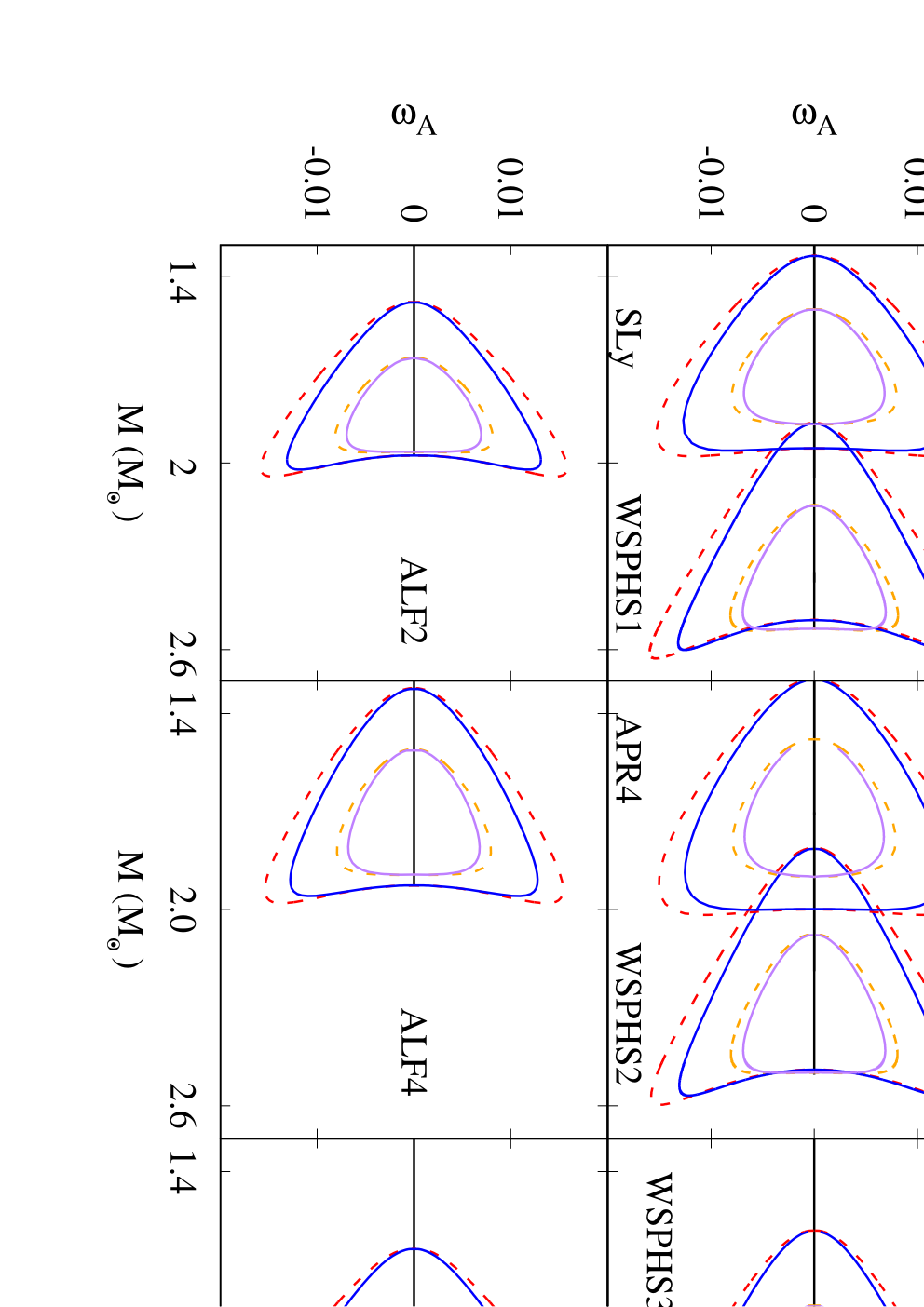
Still, as seen in Fig. 2, where the scalar field charge $\omega_{A}$ is exhibited as a function of the total mass $M$ of the stars, the general behaviour and the maximum value of the scalar charge are very similar for all EOSs – except for BS4 (where the results suggest that beyond the maximum mass, the scalarized configurations cannot be trusted). This is surprising since the EOSs describe physically widely differing systems, and it calls for further investigation to be performed in the next subsection. We note that the symmetry $\varphi\to-\varphi$ of the equations implies the symmetry $\omega_{A}\to-\omega_{A}$.

As noted above, since in the limit of small scalar field $\varphi$, the coupling functions considered are essentially the same ($A_{1}\sim A_{2}\sim 1+\frac{1}{2}\beta\varphi^{2}+...$), the branching configurations, where scalarization begins and ends, coincide for a given EOS for the coupling functions $A_{i}(\varphi)$, when the coupling parameter $\beta$ has the same value. This holds, in particular, also for the critical values $\beta_{\rm cr}$, which determine the onset of scalarization.

In Fig. 3 $\beta_{\rm cr}$ is shown versus the compactness ${\cal C}=M/R_{s}$ for all EOSs considered, except for BS4. For BS4 the onset arises at $\beta_{\rm cr}=-4.336$ and ${\cal C}=M/R_{s}=0.2193$, and thus differs $\%0.2$ in $\beta$. For all other EOSs, thus including nuclear, hyperon, hybrid and quark matter, the value of $\beta_{\rm cr}$ varies only between -4.348 and -4.343, in good agreement with the value of -4.35 given by Harada [12]. It was also noted by Harada [13] that there exists a relation between the region of scalarization and the compactness of the star. As seen in Fig. 3, the onset of scalarization can be well parametrized by the function of the compactness

with $c_{0}=-4.17789$, $c_{1}=-0.0544455$ and $c_{4}=0.000186767$, and the reduced $\chi^{2}$ is $4.3\cdot 10^{-7}$. An efficient method to obtain $\beta_{\rm cr}$ is discussed in the Appendix.

As seen in Fig. 2, the general behaviour of the scalar field is quite independent of the EOS considered, with the exception of the EOS BS4. Let us therefore now consider the mean values $E$ and the corresponding coefficients of variation ($CV$) (i.e., the ratio of the standard deviation to the mean value) of several characteristic properties of the scalar field, obtained for the full set of EOSs except for BS4. In particular, we exhibit in Table 1 for both coupling functions $A_{1}$ and $A_{2}$ and both coupling parameters $\beta_{1}$ and $\beta_{2}$ the mean value and the coefficient of variation for the maximum value of the scalar field charge $\omega_{A}$, the central value of the scalar field $\varphi_{0}$, and the surface value of the scalar field $\varphi_{s}$. Clearly, the $CV$ is rather small for all quantities.

The above analysis indicates again, that there should be some largely EOS independent agent responsible for the magnitude of the scalarization. Let us then again consider the compactness $\cal C$ and study the dependence of the scalar field on the compactness, which is the major ingredient for many universal relations. To that end we exhibit in Fig. 4 the scalar field charge $\omega_{A}$ versus the the compactness ${\cal C}=M/R_{s}$ of all neutron star models for all 14 EOSs with coupling function $A_{1}$ for $\beta=-4.5$ [Fig. 4(a)] and $\beta=-4.8$ [Fig. 4(b)].

These figures indeed reveal a certain amount of EOS independence, showing some clustering in the small $\cal C$ region for the nuclear, hyperon and hybrid EOSs. However, the two quark EOSs are distinctly offset, being shifted to higher compactness. The figures also show that the BS4 EOS follows the general trend of the nuclear, hyperon and hybrid EOSs only up to a certain compactness (close to the maximum value of the mass), where it starts to behave strangely. This possibly indicates that beyond this certain compactness this EOS may no longer be reliable in this context.

While compactness is certainly an important ingredient, it does not fully predict the onset and magnitude of the scalarization. A much better predictor of the onset and magnitude of the scalarization is the gravitational potential at the center of the star as embodied by the metric component $g_{tt}(0)=-e^{f(0)}$. Note this expression is not coordinate dependent, since the gauge freedom has been fixed by specifying the metric in Eq. (10). We have investigated the dependence of the scalar field charge $\omega_{A}$, and of the values of the scalar field at the center $\varphi(0)$ and at the surface versus the value of the metric function $g_{tt}(0)$ at the center of the star for all EOSs and both of the coupling functions. This dependence is demonstrated in Fig. 5, where we show the results for the coupling function $A_{1}$. Indeed, there is a strong universal behaviour visible, including all EOSs, also the quark EOSs. Only the BS4 EOS starts to deviate again, and should possibly no longer be trusted beyond the maximum mass.

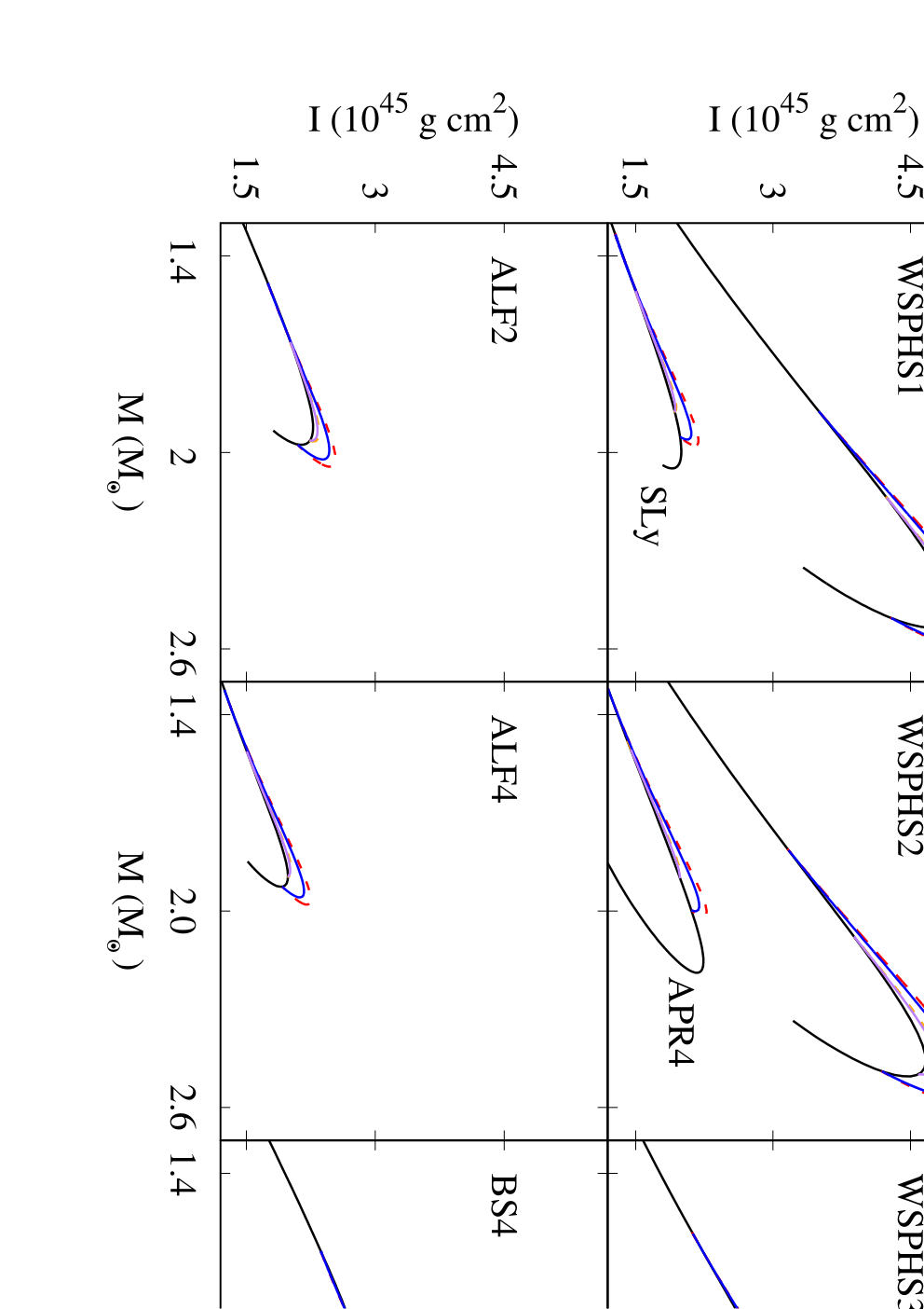
We now turn to slowly rotating neutron star models, obtained in lowest order perturbation theory. In Fig. 6 we present the moment of inertia $I$ as a function of the total mass $M$ of the neutron stars. The moment of inertia represents an important physical property of the neutron stars, since it can be obtained from timing observations of pulsars, and thus represents another observational handle to constrain the EOS of neutron stars. As seen in Fig. 6 the effect of the scalarization is to allow for somewhat larger values of the moment of inertia than in GR.

Let us now address the universality of the moment-of-inertia–compactness relations, suggested before [30, 31]

In STT these $I$-$\cal C$ relations have been considered by Staykov et al. [22], employing six purely nuclear EOSs (SLy [34], APR4 [35], FPS [47], GCP [48], Shen [49, 50] and WFF2 [51]) and two quark EOSs (SQSB40 [52] and SQSB60 [52]). We here extend their study to our full set of 14 EOSs, which, in particular, include the classes of hyperon and hybrid EOSs, not studied before in this context.

In Fig. 7 we present the moment of inertia $I$ as a function of the compactness $\cal C$, employing the two scalings $I/MR_{s}^{2}$ (a) and $I/M^{3}$ (b) for all 14 EOSs. The figures include the values for both coupling functions $A_{i}$ with $\beta_{1}$, as well as the GR values. The symbols in the figures denote the respective scaled values of $I$ versus $\cal C$, associated with the various EOSs. The colors of the symbols mark these values in the respective theories, i.e., GR (black), STT $A_{1}$, $\beta_{1}$ (red), STT $A_{2}$, $\beta_{1}$ (blue).

Besides the symbols associated with the various EOSs for the scaled values of $I$, the upper panels also show the fitted universal relations (21) and (22) as solid lines: GR (grey), STT $A_{1}$, $\beta_{1}$ (orange), STT $A_{2}$, $\beta_{1}$ (cyan). Note, that for the GR case we have included only configurations up to the maximum mass. We have not included the pure quark stars (WSPHS1 and WSPHS2) in the fits, since quark stars exhibit a somewhat different behaviour [22]. The lower panels exhibit the deviations from the fitted values, $|1-I/I_{\rm fit}|$, which are always below $10\%$.

We exhibit the fitted coefficients for both universal relations (21) and (22) in Table 2 . We find excellent agreement with the results of Staykov et al. [22]. Interestingly, the inclusion of the hyperon and hybrid EOS classes has little impact on these universal relations for the nuclear matter. Only pure quark matter is distinctly different.

Let us consider the case of a small scalar function $\varphi$, i.e., we may neglect terms of order $\varphi^{2}$. The differential equations then reduce to the equations in GR plus a linear equation for the scalar field,

Using $r=R\frac{x}{1-x}$ and $r^{2}\frac{d}{dr}=Rx^{2}\frac{d}{dx}$, we find

We note that the boundary conditions $\varphi\rvert_{x=1}=0$ and $\frac{d\varphi}{dx}\rvert_{x=0}=0$ have to be supplemented with an additional condition to guarantee a non-trivial solution. Since the ODE is linear we can choose without loss of generality $\varphi(0)=1$.

In the following we derive a simple iteration scheme to find solutions. For simplicity we write Eq. (24) in the form

with

Integration then yields

where the integration constant has been set to zero to ensure $\varphi^{\prime}(0)=0$. A second integration yields

The integration constant $c_{0}$ is determined from the boundary condition $\varphi(1)=0$, i.e.,

This leads to

Note that this is an implicit equation, since $\varphi$ appears on the rhs and the lhs of the equation. Evaluating Eq. (30) at $x=0$ yields

Since we require $\varphi(0)=1$, we have to consider $\beta$ as a dependent quantity. Solutions of Eq. (30) exist only for certain values of $\beta$.

The iteration scheme is now given by

The iterations converge very fast. Typically 10 steps are sufficient to determine $\beta$ up to 10 digits.

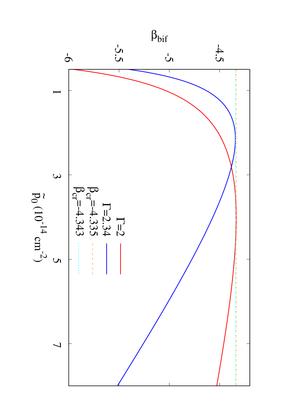
This method yields for any neutron star solution in GR the value of $\beta$ where the bifurcation of the scalarized neutron star solutions occurs. If the sequence of neutron star solutions in GR is characterized by the central pressure $\tilde{p}_{0}$, one obtains $\beta_{\rm bif}(\tilde{p}_{0})$. The maximum of $\beta_{\rm bif}(\tilde{p}_{0})$ in turn determines the critical value $\beta_{\rm cr}$ beyond which no scalarized neutron star solutions exist. The critical $\beta_{\rm cr}$ then only depends on the EOS.

To demonstrate this property we consider (for simplicity) two polytropic EOSs (16) with $K=1186.0$ and $\Gamma=2.34$, $\beta_{\rm cr}=-4.343$ and with $K=72.5216$ and $\Gamma=2.0$, $\beta_{\rm cr}=-4.335$. Fig. 8 shows $\beta_{\rm bif}$ as a function of the central pressure $\tilde{p}_{0}$. The maximal value of $\beta_{\rm bif}$ represents the critical value $\beta_{\rm cr}$ for a given EOS. For the two EOSs considered, these critical values are indicated by the horizontal lines.

In order to obtain the bifurcation points for realistic EOSs using the numerical approach described in section 2.4, we implement the following procedure: instead of iterating the integral relation (32), we solve the differential equation (24), but now assuming that $\beta=B(x)$ is a function of $x$

We thus add the following auxiliary differential equation to the system

This method is equivalent to the previous one. We have to supply three boundary conditions, which we choose to be the same as described in the previous method, $\varphi\rvert_{x=1}=0$, $\frac{d\varphi}{dx}\rvert_{x=0}=0$ and $\varphi\rvert_{x=0}=1$. This is implemented in COLSYS, together with a routine that interpolates a previously generated static solution. Static solutions with $500-1000$ points give good results. The method converges fast and works for all EOSs considered. The function $B(x)$ converges to a constant value, that determines the bifurcation point, $B(x)=\beta_{\rm bif}$. In principle, $\beta_{\rm bif}$ depends on the EOS and the central pressure of the static configuration. This approach is similar to the method used by Harada in [13] to calculate the bifurcation point using quasinormal modes, when constraining to the case of vanishing imaginary part of the fequencies.

The critical value $\beta_{\rm cr}$ is calculated as the maximum of $\beta_{\rm bif}$. In the Figures 3 and 9, the critical value $\beta_{\rm cr}$ is shown as a function of the compactness and of the trace of the energy-momentum tensor, i.e., the quantity $\tilde{\varepsilon}-3\tilde{p}_{0}$, respectively. All realistic EOSs possess very similar values of $\beta_{\rm cr}$, which may be related to the fact that all of them have similar values of the compactness ${\cal C}=M/R$ and the gravitational potential at the center as represented by $g_{tt}(0)$.

References

- [1] C. M. Will, Living Rev. Rel. 9, 3 (2006).
- [2] V. Faraoni and S. Capozziello, Fundam. Theor. Phys. 170 (2010).
- [3] E. Berti et al., Class. Quant. Grav. 32, 243001 (2015).
- [4] F. Ozel and P. Freire, Ann. Rev. Astron. Astrophys. 54, 401 (2016).
- [5] J. M. Lattimer, Ann. Rev. Nucl. Part. Sci. 62, 485 (2012).
- [6] J. A. Faber and F. A. Rasio, Living Rev. Rel. 15, 8 (2012).
- [7] C. Brans and R. H. Dicke, Phys. Rev. 124, 925 (1961).
- [8] T. Damour and G. Esposito-Farèse, Class. Quant. Grav. 9, 2093 (1992).
- [9] Fujii, Yasunori and Maeda, Kei-ichi, The Scalar-Tensor Theory of Gravitation, Cambridge University Press, Cambridge, 2003
- [10] T. Damour and G. Esposito-Farèse, Phys. Rev. Lett. 70, 2220 (1993).
- [11] T. Damour and G. Esposito-Farèse, Phys. Rev. D 54, 1474 (1996).
- [12] T. Harada, Phys. Rev. D 57, 4802 (1998).
- [13] T. Harada, Prog. Theor. Phys. 98, 359 (1997)
- [14] M. Salgado, D. Sudarsky and U. Nucamendi, Phys. Rev. D 58, 124003 (1998).
- [15] H. Sotani, Phys. Rev. D 86, 124036 (2012).
- [16] P. Pani and E. Berti, Phys. Rev. D 90, 024025 (2014).
- [17] H. O. Silva, C. F. B. Macedo, E. Berti and L. C. B. Crispino, Class. Quant. Grav. 32, 145008 (2015)
- [18] H. Sotani and K. D. Kokkotas, Phys. Rev. D 95, 044032 (2017).
- [19] D. D. Doneva, S. S. Yazadjiev, N. Stergioulas and K. D. Kokkotas, Phys. Rev. D 88, 084060 (2013).
- [20] D. D. Doneva, S. S. Yazadjiev, N. Stergioulas, K. D. Kokkotas and T. M. Athanasiadis, Phys. Rev. D 90, 044004 (2014).
- [21] D. D. Doneva, S. S. Yazadjiev, K. V. Staykov and K. D. Kokkotas, Phys. Rev. D 90, 104021 (2014).
- [22] K. V. Staykov, D. D. Doneva and S. S. Yazadjiev, Phys. Rev. D 93, 084010 (2016).
- [23] S. S. Yazadjiev, D. D. Doneva and D. Popchev, Phys. Rev. D 93, 084038 (2016).
- [24] D. D. Doneva and S. S. Yazadjiev, JCAP 1611, 019 (2016).
- [25] F. M. Ramazanoğlu and F. Pretorius, Phys. Rev. D 93, no. 6, 064005 (2016)
- [26] J. Alsing, E. Berti, C. M. Will and H. Zaglauer, Phys. Rev. D 85, 064041 (2012)
- [27] E. Berti, L. Gualtieri, M. Horbatsch and J. Alsing, Phys. Rev. D 85, 122005 (2012)
- [28] K. Yagi and N. Yunes, Phys. Rept. 681, 1 (2017).
- [29] D. Doneva and G. Pappas, “Universal relations and Alternative Gravity Theories”, submitted for publication.
- [30] J. M. Lattimer and B. F. Schutz, Astrophys. J. 629, 979 (2005).
- [31] C. Breu and L. Rezzolla, Mon. Not. Roy. Astron. Soc. 459, 646 (2016).
- [32] G. Esposito-Farèse and D. Polarski, Phys. Rev. D 63, 063504 (2001).
- [33] P. C. C. Freire et al., Mon. Not. Roy. Astron. Soc. 423, 3328 (2012).
- [34] F. Douchin and P. Haensel, Astron. Astrophys. 380, 151 (2001).
- [35] A. Akmal, V. R. Pandharipande and D. G. Ravenhall, Phys. Rev. C 58, 1804 (1998).
- [36] I. Bednarek, P. Haensel, J. L. Zdunik, M. Bejger and R. Manka, Astron. Astrophys. 543, A157 (2012).
- [37] N. K. Glendenning, Astrophys. J. 293, 470 (1985).
- [38] B. D. Lackey, M. Nayyar and B. J. Owen, Phys. Rev. D 73, 024021 (2006).
- [39] S. Weissenborn, D. Chatterjee and J. Schaffner-Bielich, Phys. Rev. C 85, 065802 (2012) Erratum: [Phys. Rev. C 90, 019904 (2014)].
- [40] S. Weissenborn, I. Sagert, G. Pagliara, M. Hempel and J. Schaffner-Bielich, Astrophys. J. 740, L14 (2011).
- [41] M. Alford, M. Braby, M. W. Paris and S. Reddy, Astrophys. J. 629, 969 (2005).
- [42] L. Bonanno and A. Sedrakian, Astron. Astrophys. 539, A16 (2012).
- [43] P. Demorest, T. Pennucci, S. Ransom, M. Roberts and J. Hessels, Nature 467, 1081 (2010).
- [44] J. Antoniadis et al., Science 340, 6131 (2013).
- [45] U. Ascher, J. Christiansen and R. D. Russell, Math. Comput. 33, 659 (1979).
- [46] J. S. Read, B. D. Lackey, B. J. Owen and J. L. Friedman, Phys. Rev. D 79, 124032 (2009).
- [47] C. P. Lorenz, D. G. Ravenhall and C. J. Pethick, Phys. Rev. Lett. 70, 379 (1993).
- [48] S. Goriely, N. Chamel and J. M. Pearson, Phys. Rev. C 82, 035804 (2010).
- [49] H. Shen, H. Toki, K. Oyamatsu and K. Sumiyoshi, Nucl. Phys. A 637, 435 (1998).
- [50] H. Shen, H. Toki, K. Oyamatsu and K. Sumiyoshi, Prog. Theor. Phys. 100, 1013 (1998).
- [51] R. B. Wiringa, V. Fiks and A. Fabrocini, Phys. Rev. C 38, 1010 (1988).
- [52] D. Gondek-Rosinska and F. Limousin, arXiv:0801.4829 [gr-qc].
- [53] B. Kleihaus, J. Kunz and S. Yazadjiev, Phys. Lett. B 744, 406 (2015)