跳到论文正文
W Papers独立论文阅读器 arXiv:1707.05222 论文正文 计算阅读时间 · 0%
引用这篇论文根据当前论文元数据生成,正式投稿前建议核对。


License: CC BY-SA 4.0
arXiv:1707.05222v3 [math.CA] 06 Jan 2018

Poles of Painlevé IV Rationals and their Distribution

This paper is a contribution to the Special Issue on Painlevé Equations and Applications in Memory of Andrei Kapaev. The full collection is available at https://www.emis.de/journals/SIGMA/Kapaev.html
Davide MASOERO † and Pieter ROFFELSEN ‡
Abstract

We study the distribution of singularities (poles and zeros) of rational solutions of the Painlevé IV equation by means of the isomonodromic deformation method. Singularities are expressed in terms of the roots of generalised Hermite Hm,nH_{m,n} and generalised Okamoto Qm,nQ_{m,n} polynomials. We show that roots of generalised Hermite and Okamoto polynomials are described by an inverse monodromy problem for an anharmonic oscillator of degree two. As a consequence they turn out to be classified by the monodromy representation of a class of meromorphic functions with a finite number of singularities introduced by Nevanlinna. We compute the asymptotic distribution of roots of the generalised Hermite polynomials in the asymptotic regime when mm is large and nn fixed.

keywords
Painlevé fourth equation; singularities of Painlevé transcendents; isomonodromic deformations; generalised Hermite polynomials; generalised Okamoto polynomials
AMS
34M55; 34M56; 34M60; 33C15; 30C15
††shorttitle: Poles of Painlevé IV Rationals and their Distribution††runningauthor: D. Masoero and P. Roffelsen††address: † Grupo de Física Matemática e Departamento de Matemática da Universidade de Lisboa,
† Campo Grande Edifício C6, 1749-016 Lisboa, Portugal
††email: dmasoero@gmail.com††url: http://gfm.cii.fc.ul.pt/people/dmasoero/††address: ‡ School of Mathematics and Statistics F07, The University of Sydney, NSW 2006, Australia††email: p.roffelsen@maths.usyd.edu.au††dates: Received July 20, 2017, in final form December 18, 2017; Published online January 06, 2018

To the memory of Andrei A. Kapaev, a master of Painlevé equations, untiring author, referee and reviewer.

1 Introduction

In this paper we address, by means of the isomonodromic deformation method [22, 27, 28], the distribution of movable singularities (which are zeros and poles) of rational solutions of the fourth Painlevé equation, also called Painlevé IV and denoted by PIV{\rm P}_{\rm IV}, which is the following second order differential equation,

ωz​z=12​ω​ωz2+32​ω3+4​z​ω2+2​(z2+1−2​θ∞)​ω−8​θ02ω,θ:=(θ0,θ∞)∈ℂ2.\displaystyle\omega_{zz}=\displaystyle\frac{1}{2\omega}\omega_{z}^{2}+\frac{3}{2}\omega^{3}+4z\omega^{2}+2\big(z^{2}+1-2\theta_{\infty}\big)\omega-\frac{8\theta_{0}^{2}}{\omega},\qquad\theta:=(\theta_{0},\theta_{\infty})\in\mathbb{C}^{2}. (1.1)

We sometimes write PIV​(θ){\rm P}_{\rm IV}(\theta) to stipulate the particular parameter values in consideration.

PIV{\rm P}_{\rm IV} is one of the famous six Painlevé equations, all of which have had an enormous impact in several branches of science, including mathematical physics, algebraic geometry, applied mathematics, fluid dynamics and statistical mechanics, see, e.g., [11, 12, 23] and references therein.

Special solutions, such as rational solutions, and the distribution of movable singularities have proven to be particularly important in applications and were thoroughly studied by means of ad-hoc methods which are unavailable for regular values or generic solutions; see, e.g., [2, 9, 13, 37, 45] and references therein. In the case under consideration, we will show that singularities of rational solutions of Painlevé IV are characterised by the monodromy representation of three particular classes of meromorphic functions (introduced by Nevanlinna [44]) with a finite number of critical points and transcendental singularities.

One of the most striking features of solutions of Painlevé equations is that their value distributions are often observed to describe some approximate lattice structure, as was first discovered by Boutroux [3] for solutions of Painlevé I and II. This is also the case for singularities of Painlevé IV rationals. Indeed one of the main inspirations of our work is the highly regular pattern of their distribution, which was observed by Clarkson [8] (see [51] for more general solutions), and which has so far eluded any rigorous clarification. By computing the distribution of singularities in a particular asymptotic regime we furnish here the first rigorous, albeit partial, explanation11 1 We notice that the same question for Painlevé II rationals has recently been settled by many authors with a wealth of different methods [2, 5, 6, 41, 52, 53]..

For the sake of clarity of our exposition, before introducing our main results together with an outline of the article, we briefly review some well-known facts from the theory of movable singularities and rational solutions of Painlevé IV.

1.1 Zeros and poles of solutions

The Painlevé property implies that any local solution of PIV{\rm P}_{\rm IV} has a unique meromorphic continuation to the entire complex plane [55]. As a consequence the solution space is the set of meromorphic functions on ℂ\mathbb{C} that satisfy (1.1), which we denote by

𝒲θ={PIV​(θ)​transcendents}.\displaystyle\mathcal{W}_{\theta}=\{{\rm P}_{\text{IV}}(\theta)\ \text{transcendents}\}. (1.2)

Upon fixing an a∈ℂa\in\mathbb{C}, any Painlevé IV transcendent (i.e., solution) enjoys a Laurent expansion at this point. In particular the generic Laurent expansion takes the form

ω⁡(z)=b+c⁡(z−a)+ω2​(z−a)2+ω3​(z−a)3+𝒪⁡((z−a)4),\displaystyle\omega(z)=b+c(z-a)+\omega_{2}(z-a)^{2}+\omega_{3}(z-a)^{3}+\mathcal{O}\big((z-a)^{4}\big), (1.3)

for b∈ℂ∗b\in\mathbb{C}^{*} and c∈ℂc\in\mathbb{C}, where the higher order coefficients are of the form ωn=1b​pn\omega_{n}=\frac{1}{b}p_{n}, with pnp_{n} polynomial in aa, bb, cc, θ\theta for n≥2n\geq 2. However this expansion breaks down when ω⁡(a)∈{0,∞}\omega(a)\in\{0,\infty\}, i.e., ω\omega has a zero or pole at z=az=a, in which case the Laurent expansions take the respective forms

ω⁡(z)=4​ϵ​θ0​(z−a)+b​(z−a)2+ω3​(z−a)3+𝒪⁡((z−a)4),ϵ=±1,\displaystyle\omega(z)=4\epsilon\theta_{0}(z-a)+b(z-a)^{2}+\omega_{3}(z-a)^{3}+\mathcal{O}\big((z-a)^{4}\big),\qquad\epsilon=\pm 1, (1.4)

where we refer to the value of ϵ\epsilon as the sign of the zero, or

ω⁡(z)=ϵz−a−a+ω1​(z−a)+b​(z−a)2+ω3​(z−a)3+𝒪⁡((z−a)4),ϵ=±1,\displaystyle\omega(z)=\frac{\epsilon}{z-a}-a+\omega_{1}(z-a)+b(z-a)^{2}+\omega_{3}(z-a)^{3}+\mathcal{O}\big((z-a)^{4}\big),\qquad\epsilon=\pm 1, (1.5)

where ω1=13​ϵ​(a2−2+4​(θ∞−ϵ))\omega_{1}=\tfrac{1}{3}\epsilon(a^{2}-2+4(\theta_{\infty}-\epsilon)), in both cases b∈ℂb\in\mathbb{C}, and all higher order coefficients have polynomial dependence on aa, bb, θ\theta; conversely, for any choice of parameters the Laurent series (1.3)–(1.5) converge locally to a solution of PIV{\rm P}_{\rm IV}. Indeed, one can find a positive constant Ca,bC_{a,b} such that |ωn|≤Ca,bn|\omega_{n}|\leq C_{a,b}^{n}, for n≥3n\geq 3, and thus the formal power-series actually has a non-zero radius of convergence, see, e.g., [21, 26].

From an algebro-geometric point of view [29, 48], it is clear that zeros and poles of PIV{\rm P}_{\rm IV} transcendents play a fundamentally distinguished role; they are the movable singularities of solutions.

1.2 Rational solutions

Firstly, let us remark that PIV{\rm P}_{\rm IV} enjoys various Bäcklund transformations, which relate solutions with different parameter values. In particular we have transformations ℛ1\mathcal{R}_{1}–ℛ4\mathcal{R}_{4}, see Appendix B for their definitions, which allow us to relate the solution spaces 𝒲θ\mathcal{W}_{\theta} and 𝒲θ′\mathcal{W}_{\theta^{\prime}} whenever θ−θ′∈ℤ2∪(ℤ+12)2\theta-\theta^{\prime}\in\mathbb{Z}^{2}\cup(\mathbb{Z}+\tfrac{1}{2})^{2}.

Painlevé IV admits a rational solution if and only if the parameters satisfy either

θ∞∈12​ℤ,θ0−θ∞∈ℤ,\displaystyle\theta_{\infty}\in\tfrac{1}{2}\mathbb{Z},\qquad\theta_{0}-\theta_{\infty}\in\mathbb{Z}, (1.6)

or

θ∞∈12​ℤ,θ0−θ∞∈ℤ±23.\displaystyle\theta_{\infty}\in\tfrac{1}{2}\mathbb{Z},\qquad\theta_{0}-\theta_{\infty}\in\mathbb{Z}\pm\tfrac{2}{3}. (1.7)

Furthermore for any such parameter values the associated rational solution is unique [25, 34, 43]. Using the τ\tau-function formalism, Noumi and Yamada [46] expressed these rational solutions conveniently in terms of generalised Hermite Hm,n​(z)H_{m,n}(z) and generalised Okamoto polynomials Qm,n​(z)Q_{m,n}(z), see Appendix A for their precise definition.

Firstly, the parameter cases (1.6), up to equivalence θ0↔−θ0\theta_{0}\leftrightarrow-\theta_{0}, are given by

ωm,n(I)=dd​z​log⁡Hm+1,nHm,n,\displaystyle\omega_{m,n}^{({\rm I})}=\frac{{\rm d}}{{\rm d}z}\log\frac{H_{m+1,n}}{H_{m,n}},\quad θ0=12​n,\displaystyle\theta_{0}=\tfrac{1}{2}n,\quad θ∞=m+12​n+1,\displaystyle\theta_{\infty}=m+\tfrac{1}{2}n+1, (1.8a)
ωm,n(II)=dd​z​log⁡Hm,nHm,n+1,\displaystyle\omega_{m,n}^{({\rm II})}=\frac{{\rm d}}{{\rm d}z}\log\frac{H_{m,n}}{H_{m,n+1}},\quad θ0=12​m,\displaystyle\theta_{0}=\tfrac{1}{2}m,\quad θ∞=−12​m−n,\displaystyle\theta_{\infty}=-\tfrac{1}{2}m-n, (1.8b)
ωm,n(III)=−2​z+dd​z​log⁡Hm,n+1Hm+1,n,\displaystyle\omega_{m,n}^{({\rm III})}=-2z+\frac{{\rm d}}{{\rm d}z}\log\frac{H_{m,n+1}}{H_{m+1,n}},\quad\ \ θ0=12​(m+n+1),\displaystyle\theta_{0}=\tfrac{1}{2}(m+n+1),\quad\ θ∞=12​(n−m+1),\displaystyle\theta_{\infty}=\tfrac{1}{2}(n-m+1), (1.8c)

where m,n∈ℕm,n\in\mathbb{N}, which we refer to as the Hermite I, II and III families respectively. Some particularly simple members of these respective families are

ω0,1(I)=1z,\displaystyle\omega_{0,1}^{({\rm I})}=\frac{1}{z},\qquad θ0=12,\displaystyle\theta_{0}=\tfrac{1}{2},\qquad θ∞=32,\displaystyle\theta_{\infty}=\tfrac{3}{2}, (1.9a)
ω1,0(II)=−1z,\displaystyle\omega_{1,0}^{({\rm II})}=-\frac{1}{z},\qquad θ0=12,\displaystyle\theta_{0}=\tfrac{1}{2},\qquad θ∞=−12,\displaystyle\theta_{\infty}=-\tfrac{1}{2}, (1.9b)
ω0,0(III)=−2​z,\displaystyle\omega_{0,0}^{({\rm III})}=-2z,\qquad θ0=12,\displaystyle\theta_{0}=\tfrac{1}{2},\qquad θ∞=12,\displaystyle\theta_{\infty}=\tfrac{1}{2}, (1.9c)

and the other ones can be obtained via application of the Bäcklund transformations ℛ1\mathcal{R}_{1}–ℛ4\mathcal{R}_{4}, as depicted in Table 1.

ωm,n(I)\omega_{m,n}^{({\rm I})} ωm,n(II)\omega_{m,n}^{({\rm II})} ωm,n(III)\omega_{m,n}^{({\rm III})} ω~m,n\widetilde{\omega}_{m,n}
ℛ1\mathcal{R}_{1} ωm+1,n−1(I)\omega_{m+1,n-1}^{({\rm I})} ωm−1,n(II)\omega_{m-1,n}^{({\rm II})} ωm−1,n(III)\omega_{m-1,n}^{({\rm III})} ω~m+1,n−1\widetilde{\omega}_{m+1,n-1}
ℛ2\mathcal{R}_{2} ωm−1,n+1(I)\omega_{m-1,n+1}^{({\rm I})} ωm+1,n(II)\omega_{m+1,n}^{({\rm II})} ωm+1,n(III)\omega_{m+1,n}^{({\rm III})} ω~m−1,n+1\widetilde{\omega}_{m-1,n+1}
ℛ3\mathcal{R}_{3} ωm,n+1(I)\omega_{m,n+1}^{({\rm I})} ωm+1,n−1(II)\omega_{m+1,n-1}^{({\rm II})} ωm,n+1(III)\omega_{m,n+1}^{({\rm III})} ω~m,n+1\widetilde{\omega}_{m,n+1}
ℛ4\mathcal{R}_{4} ωm,n−1(I)\omega_{m,n-1}^{({\rm I})} ωm−1,n+1(II)\omega_{m-1,n+1}^{({\rm II})} ωm,n−1(III)\omega_{m,n-1}^{({\rm III})} ω~m,n−1\widetilde{\omega}_{m,n-1}
Table 1: Action of Bäcklund transformations on rational solutions of PIV{\rm P}_{\rm IV}.

Secondly, the parameter cases (1.7), up to equivalence θ0↔−θ0\theta_{0}\leftrightarrow-\theta_{0}, are given by

ω~m,n=−23​z+dd​z​log⁡Qm+1,nQm,n,θ0=−16+12​n,θ∞=12​(2​m+n+1),\displaystyle\widetilde{\omega}_{m,n}=-\frac{2}{3}z+\frac{{\rm d}}{{\rm d}z}\log\frac{Q_{m+1,n}}{Q_{m,n}},\qquad\theta_{0}=-\tfrac{1}{6}+\tfrac{1}{2}n,\qquad\theta_{\infty}=\tfrac{1}{2}(2m+n+1), (1.10)

where m,n∈ℤm,n\in\mathbb{Z}, which we refer to as the Okamoto family. A particularly simple member of the Okamoto family, is given by

ω~0,0=−23​z,θ0=−16,θ∞=12.\displaystyle\widetilde{\omega}_{0,0}=-\tfrac{2}{3}z,\qquad\theta_{0}=-\tfrac{1}{6},\qquad\theta_{\infty}=\tfrac{1}{2}.

and again the other ones can be obtained via application of the Bäcklund transformations ℛ1\mathcal{R}_{1}–ℛ4\mathcal{R}_{4}, as Table 1 shows.

Remarkably, all zeros and poles of rational solutions can be expressed as roots of the generalised Hermite and Okamoto polynomials, see Table 2. Therefore the study of the distribution of movable singularities of PIV{\rm P}_{\text{IV}} rationals is reduced to that of zeros of the generalised Hermite and Okamoto polynomials.

zeros (ϵ=+1\epsilon=+1) zeros (ϵ=−1\epsilon=-1) poles (ϵ=+1\epsilon=+1) poles (ϵ=−1\epsilon=-1)
ωm,n(I)\omega_{m,n}^{({\rm I})} Hm+1,n−1H_{m+1,n-1} Hm,n+1H_{m,n+1} Hm+1,nH_{m+1,n} Hm,nH_{m,n}
ωm,n(II)\omega_{m,n}^{({\rm II})} Hm−1,n+1H_{m-1,n+1} Hm+1,nH_{m+1,n} Hm,nH_{m,n} Hm,n+1H_{m,n+1}
ωm,n(III)\omega_{m,n}^{({\rm III})} Hm,nH_{m,n} Hm+1,n+1H_{m+1,n+1} Hm,n+1H_{m,n+1} Hm+1,nH_{m+1,n}
ω~m,n\widetilde{\omega}_{m,n} Qm+1,n−1Q_{m+1,n-1} Qm,n+1Q_{m,n+1} Qm+1,nQ_{m+1,n} Qm,nQ_{m,n}
Table 2: The zeros and poles of rational solutions in terms of generalised Hermite and Okamoto polynomials. As an example, poles with residue ε=+1\varepsilon=+1 of ωm,n(III)\omega_{m,n}^{({\rm III})} coincide with the roots of Hm,n+1H_{m,n+1}. The table is computed using equations (1.8) and (1.10) and the action of the Bäcklund transformations (B.1).

1.3 Outline and main results

In Section 2 we recall the isomonodromic deformation interpretation of Painlevé IV, via the Garnier–Jimbo–Miwa Lax pair. The Riemann–Hilbert correspondence associates bijectively any solution of Painlevé IV to a unique monodromy datum of the Garnier–Jimbo–Miwa linear system; given a point zz in the complex plane and a solution ω\omega of PIV{\rm P}_{\rm IV}, the inverse monodromy problem furnishes the value ω⁡(z)\omega(z) unless zz is a zero or a pole, in which cases the inverse monodromy problem for the linear system does not have any solution.

However, following [37], we show that the inverse monodromy problem can be defined in case of zeros and poles, and in fact it simplifies to that of the anharmonic oscillator

ψ′′​(λ)=V⁡(λ,a,b,θ)​ψ​(λ),\displaystyle\psi^{\prime\prime}(\lambda)=V(\lambda;a,b,\theta)\psi(\lambda),
V⁡(λ,a,b,θ)=λ2+2​a​λ+a2+2​(1−θ∞)−[b+(2​θ∞−12)​a]​λ−1+(θ02−14)​λ−2.\displaystyle V(\lambda;a,b,\theta)=\lambda^{2}+2a\lambda+a^{2}+2(1-\theta_{\infty})-\big[b+\big(2\theta_{\infty}-\tfrac{1}{2}\big)a\big]\lambda^{-1}+\big(\theta_{0}^{2}-\tfrac{1}{4}\big)\lambda^{-2}.

The main result of this section is that the aforementioned simplification allows us the characterise zeros and poles of rational solutions exactly as the solutions of an inverse monodromy problem concerning the anharmonic oscillator in question; see Theorem 2.2.

According to the beautiful theory developed by Nevanlinna and his school [14, 44], anharmonic oscillators (in case all singularities in the complex plane are Fuchsian and apparent) naturally define Riemann surfaces which are infinitely-sheeted coverings of the Riemann sphere uniformised by meromorphic functions. In Section 3 we define three families of such Nevanlinna functions and show how they classify the zeros and poles of rational solutions. This characterisation is rather powerful, as an easy corollary gives us the solution to a previously open problem, namely to determine exactly the number of real roots of the generalised Hermite polynomials; see Corollary 3.5.

Finally, in Section 4 we study the asymptotic distribution of zeros of the generalised Hermite polynomials Hm,nH_{m,n}, and hence zeros and poles of corresponding rational solutions in the asymptotic regime m→∞m\to\infty and nn bounded. In order to state precisely our main result we need to introduce some new notation and functions. First of all, as we will find that the roots grow like (2​m+n)12(2m+n)^{\frac{1}{2}}, it is convenient in our analysis to work with the new unknown α\alpha and ‘big parameter’ EE, defined by

α=E−12​a,E=2​m+n.\displaystyle\alpha=E^{-\frac{1}{2}}a,\qquad E=2m+n. (1.11)

The m⋅nm\cdot n roots of Hm,n​(z)H_{m,n}(z) turn out to be organised in nn approximately horizontal lines. We parametrise these lines by the set

Jn:={−n+1,−n+3,…,n−3,n−1},\displaystyle J_{n}:=\{-n+1,-n+3,\dots,n-3,n-1\},

and introduce the real functions

f:\displaystyle f\colon\ [−1,1]→[−π4,π4],\displaystyle[-1,1]\to[-\tfrac{\pi}{4},\tfrac{\pi}{4}],\qquad f⁡(x)=12​(x​(1−x2)12−cos−1⁡(x))+π4,\displaystyle f(x)=\tfrac{1}{2}\big(x(1-x^{2})^{\frac{1}{2}}-\cos^{-1}(x)\big)+\frac{\pi}{4},
gj,E:\displaystyle g_{j,E}\colon\ (−1,1)→ℝ,\displaystyle(-1,1)\to\mathbb{R},\qquad gj,E​(x)=2​j​log⁡(2​E12​(1−x2)34)−log⁡Fn,j2​E​(1−x2)12,\displaystyle g_{j,E}(x)=\frac{2j\log\big(2E^{\frac{1}{2}}\big(1-x^{2}\big)^{\frac{3}{4}}\big)-\log F_{n,j}}{2E(1-x^{2})^{\frac{1}{2}}},

where j∈Jnj\in J_{n} and the constant Fn,jF_{n,j} is defined by

Fn,j=Γ​[12​(1+n+j)]Γ​[12​(1+n−j)].\displaystyle F_{n,j}=\frac{\Gamma\big[\tfrac{1}{2}(1+n+j)\big]}{\Gamma\big[\tfrac{1}{2}(1+n-j)\big]}. (1.12)

Notice that ff is strictly monotone and therefore globally invertible. Finally, we define our approximate (rescaled) roots α\alpha.

Definition 1.1.

For every kk, with |k|≤E4|k|\leq\frac{E}{4} and kk integer if mm is odd or half-integer if mm is even, and every j∈Jnj\in J_{n}, we define the approximate root αj,k=αR+i​αI\alpha_{j,k}=\alpha_{R}+i\alpha_{I}, with αR,αI∈ℝ\alpha_{R},\alpha_{I}\in\mathbb{R}, as the unique complex number determined by the following relations

f⁡(αR)=π​kE,αR∈(−1,1),\displaystyle f(\alpha_{R})=\frac{\pi k}{E},\qquad\alpha_{R}\in(-1,1), (1.13a)
αI=gj,E​(αR).\displaystyle\alpha_{I}=g_{j,E}(\alpha_{R}). (1.13b)

The points αj,k\alpha_{j,k} are the dominant term in the asymptotic expansion of the (rescaled) roots belonging to the ’bulk’, as it is pictorially illustrated in Fig. 1 below.

Refer to caption
Refer to caption
Figure 1: Rescaled roots of H40,5H_{40,5}. In blue numerically exact location, in red the asymptotic approximation αj,k\alpha_{j,k}. In purple the curves ℑ⁡α=gj,E​(ℜ⁡α)\Im\alpha=g_{j,E}(\Re\alpha), E=85E=85, j∈J5j\in J_{5}.

We consider two cases of ’bulk’ behaviour. In the first case we compute the error in the approximation when we limit the real part of the roots to a fixed closed subinterval of (−1,1)(-1,1).

Theorem 1.2.

Fix 0<σ<140<\sigma<\frac{1}{4}. There exist a constant E0E_{0} and a constant CσC_{\sigma} such that, if E≥E0E\geq E_{0}, then for all |k|≤σ​E|k|\leq\sigma E, the polynomial Hm,n​(z)H_{m,n}(z) has one and only one zero in each disc of the form |z−E12​αj,k|≤Cσ​E−56\big|z-E^{\frac{1}{2}}\alpha_{j,k}\big|\leq C_{\sigma}E^{-\frac{5}{6}}.

In the second case, we suppose that the real part of the (rescaled) roots belong to a closed subinterval of (−1,1)(-1,1), which is growing to the full interval at some restricted rate, as EE becomes large. An interval of the kind [−1+c​E−1+δ,1−c​E−1+δ]\big[{-}1+cE^{-1+\delta},1-cE^{-1+\delta}\big] for some c>0c>0 and δ>13\delta>\frac{1}{3}.

Theorem 1.3.

Fix 13<δ≤1\frac{1}{3}<\delta\leq 1 and s>0s>0. There exist a constant E0E_{0} and a constant CsC_{s} such that, if E≥E0E\geq E_{0}, then for all |k|≤(14−s​E−32​(1−δ))​E|k|\leq\big(\frac{1}{4}-sE^{-\frac{3}{2}(1-\delta)}\big)E, the polynomial Hm,n​(z)H_{m,n}(z) has one and only one zero in each disc of the form |z−E12​αj,k|≤Cs​E−δ+16|z-E^{\frac{1}{2}}\alpha_{j,k}|\leq C_{s}E^{-\delta+\frac{1}{6}}.

In Fig. 2 the error estimates in Theorems 1.2 and 1.3 are visualised. In particular they showcase that the bounds are optimal.

Refer to caption Refer to caption Refer to caption Refer to caption
m=8m=8 m=16m=16 m=100m=100 m=144m=144

Bulk. Rescaled asymptotic approximation α4,k\alpha_{4,k} of root of Hm,5​(E12​z)H_{m,5}\big(E^{\frac{1}{2}}z\big) in red, encircled with a circle of radius Cσ​E−43C_{\sigma}E^{-\frac{4}{3}}, where Cσ=13C_{\sigma}=\tfrac{1}{3} and k:=m+24∼18​Ek:=\frac{m+2}{4}\sim\tfrac{1}{8}E as E→∞E\rightarrow\infty, for ranging values of mm. In blue the corresponding numerically exact location, confirming the error estimate in Theorem 1.2.

Refer to caption Refer to caption Refer to caption Refer to caption
m=8m=8 m=16m=16 m=100m=100 m=144m=144

Approaching the edge. Asymptotic approximation α4,k\alpha_{4,k} of root of Hm,5​(E12​z)H_{m,5}\big(E^{\frac{1}{2}}z\big) in red, encircled with two circles of radii Cσ​E−43C_{\sigma}E^{-\frac{4}{3}} and Cs​E−1C_{s}E^{-1}, where Cσ=Cs=112C_{\sigma}=C_{s}=\tfrac{1}{12} and k:=⌊14​E−E12⌋+12∼14​Ek:=\big\lfloor\tfrac{1}{4}E-E^{\frac{1}{2}}\big\rfloor+\tfrac{1}{2}\sim\tfrac{1}{4}E as E→∞E\rightarrow\infty, for ranging values of mm. In blue the corresponding numerically exact location, confirming the error estimate in Theorem 1.3 with s=1s=1 and δ=23\delta=\tfrac{2}{3}.

Figure 2: Graphical illustration of errors in Theorems 1.2 and 1.3.

We end the introduction with a few remarks on our asymptotic results.

Remark 1.4.

Notice that equation (1.13a) for the location of the real part of the zeros of Hm,n​(z)H_{m,n}(z) coincides with the equation describing the asymptotic location of the zeros of the standard Hermite polynomials [16, Section 10.17].

Remark 1.5.

Suppose that the index kk in αj,k\alpha_{j,k} is bounded by a number independent on EE, namely |k|≤k0|k|\leq k_{0} for some k0∈ℕk_{0}\in\mathbb{N}, then the points αj,k\alpha_{j,k} belong to the regular lattice

αR=k​πE+𝒪⁡(E−2),αI=j​log⁡(2​E12)−12​log⁡Fn,jE+𝒪⁡(E−2),\displaystyle\alpha_{R}=\frac{k\pi}{E}+\mathcal{O}\big(E^{-2}\big),\qquad\alpha_{I}=\frac{j\log\big(2E^{\frac{1}{2}}\big)-\frac{1}{2}\log F_{n,j}}{E}+\mathcal{O}\big(E^{-2}\big),

in the large EE limit. This explains the lattice-like pattern numerically observed in [8].

Remark 1.6.

Our approximation scheme includes all zeros, except for a set which asymptotically has probability measure zero. Indeed let N⁡(A,B)N(A,B) be the counting function for −∞<A≤B<∞-\infty<A\leq B<\infty defined as follows: set NE​(A,B)N_{E}(A,B) equal to the number of rescaled roots whose real part belong to the interval [A,B][A,B], divided by m=E−n2m=\frac{E-n}{2}, and define N⁡(A,B)=limE→∞NE​(A,B)N(A,B)=\lim\limits_{E\to\infty}N_{E}(A,B). An easy computation, based on the identity f′​(x)=1−x2f^{\prime}(x)=\sqrt{1-x^{2}}, shows that

N⁡(A,B)=∫AB2​nπ​1−x2​χ[−1,1]​(x)​𝑑x.\displaystyle N(A,B)=\int_{A}^{B}\frac{2n}{\pi}\sqrt{1-x^{2}}\chi_{[-1,1]}(x){\rm d}x.

Here χ[−1,1]\chi_{[-1,1]} is the characteristic function of the interval [−1,1][-1,1]. This is a manifestation of Wigner’s celebrated semi-circle law. This behaviour was conjectured in [20].

Remark 1.7.

Even though after Theorems 1.2 and 1.3 the bulk of the interval (−1,1)(-1,1) contains the real part of almost all roots of the generalised Hermite polynomials in the asymptotic regime under consideration, there are roots which converge to the edge of the fundamental domain too fast for the hypothesis of Theorem 1.3. In fact, their real part coalesce with ±1\pm 1 with speed E−23E^{-\frac{2}{3}}. These roots will be briefly discussed in Section 4.6 at the end of the paper where we show that their distribution is governed by an Airy-like behaviour.

Remark 1.8.

While we were finalising the present paper, the paper [4] by R. Buckingham appeared on the arXiv. This contains the asymptotic analysis, in the regime m→∞m\to\infty, mn=r\frac{m}{n}=r, of rational solutions of Hermite type in the ‘pole-free’ region. Even though [4] does not address the distribution of poles and zeros, it contests the results of [47] about the distribution of singularities in the regime m=n≫0m=n\gg 0. The paper [47] was however already peer-reviewed. Since we are not able to judge on this matter, we await for the answer of its authors.

2 Poles of rational solutions and anharmonic oscillators

It is well-known that Painlevé equations can be realised as isomonodromic deformations of linear systems. This section is dedicated to, using aforementioned formalism, giving an exact characterisation of poles of rational solutions in terms of anharmonic oscillators satisfying some prescribed constraints. Let us consider the following quadratic oscillators with centrifugal terms,

ψ′′​(λ)=V⁡(λ,a,b,θ)​ψ​(λ),\displaystyle\psi^{\prime\prime}(\lambda)=V(\lambda;a,b,\theta)\psi(\lambda),
V⁡(λ,a,b,θ)=λ2+2​a​λ+a2+2​(1−θ∞)−[b+(2​θ∞−12)​a]​λ−1+(θ02−14)​λ−2,\displaystyle V(\lambda;a,b,\theta)=\lambda^{2}+2a\lambda+a^{2}+2(1-\theta_{\infty})-\big[b+\big(2\theta_{\infty}-\tfrac{1}{2}\big)a\big]\lambda^{-1}+\big(\theta_{0}^{2}-\tfrac{1}{4}\big)\lambda^{-2}, (2.1)

where a,b∈ℂa,b\in\mathbb{C} and θ=(θ0,θ∞)∈ℂ∗×ℂ\theta=(\theta_{0},\theta_{\infty})\in\mathbb{C}^{*}\times\mathbb{C}. Without loss of generality, we may always assume ℜ⁡[θ0]≥0\Re[\theta_{0}]\geq 0, because of the invariance of (2.1) under θ0↦−θ0\theta_{0}\mapsto-\theta_{0}.

Now note that λ=0\lambda=0 is a regular singular point with indices 12±θ0\tfrac{1}{2}\pm\theta_{0}, and there generically exist two linearly independent solutions ψ±​(λ)\psi_{\pm}(\lambda), with corresponding Frobenius expansions, uniquely defined by the asymptotic behaviour at zero. However, in the resonant case θ0=12​n∈12​ℕ∗\theta_{0}=\tfrac{1}{2}n\in\tfrac{1}{2}\mathbb{N}^{*}, the Frobenius expansion of the dominant solution is not uniquely defined by its behaviour in zero ψ−​(λ)∼λ12−θ0\psi_{\scalebox{0.6}[1.0]{$-$}}(\lambda)\sim\lambda^{\frac{1}{2}-\theta_{0}} as λ→0\lambda\rightarrow 0, and logarithmic terms may appear. Indeed, we have

ψ+​(λ)=λ12+θ0​(1+𝒪⁡(λ)),λ→0,\displaystyle\psi_{+}(\lambda)=\lambda^{\tfrac{1}{2}+\theta_{0}}(1+\mathcal{O}(\lambda)),\qquad\lambda\rightarrow 0,
ψ−​(λ)=c​log⁡(λ)​ψ+​(λ)+λ12−θ0​(1+∑k≥1ck​λk),\displaystyle\psi_{-}(\lambda)=c\log(\lambda)\psi_{+}(\lambda)+\lambda^{\tfrac{1}{2}-\theta_{0}}\bigg(1+\sum_{k\geq 1}c_{k}\lambda^{k}\bigg),

where the constant cc and ckc_{k}’s are uniquely defined by imposing cn=0c_{n}=0.

For convenience of the reader we recall the definition of an apparent singularity, a concept of remarkable importance for the rest of the paper.

Definition 2.1.

A resonant regular singularity of a second order linear ODE is called apparent, if the dominant solution ψ+\psi_{+} does not have any logarithmic contribution.

Similarly, in the case of a first order system of linear ODEs, we say that a regular singularity is apparent, if the monodromy about the singularity is a scalar multiple of the identity.

In turn, equation (2.1) has an irregular singularity at λ=∞\lambda=\infty, hence solutions exhibit the Stokes phenomenon, which we discuss briefly. For each k∈ℤ4k\in\mathbb{Z}_{4}, we define the Stokes sector Ωk=ek​π​i4​Ω0\Omega_{k}=e^{\frac{k\pi i}{4}}\Omega_{0}, where Ω0={−π4<argλ<π4}\Omega_{0}=\{-\frac{\pi}{4}<\arg{\lambda}<\frac{\pi}{4}\}. In each Stokes sector there exists an (up to normalisation) unique subdominant solution ψk​(λ)\psi_{k}(\lambda), which decays exponentially as λ→∞\lambda\rightarrow\infty in this sector.

Fixing the principal branch for powers of λ\lambda in the λ\lambda-plane, with respect to the branch cut arg⁡λ=−π4\arg{\lambda}=-\frac{\pi}{4}, and denoting

g⁡(λ,z)=12​λ2+z​λ,\displaystyle g(\lambda,z)=\tfrac{1}{2}\lambda^{2}+z\lambda, (2.2)

we fix the following normalisation of the subdominant solution ψk​(λ)\psi_{k}(\lambda),

ψk​(λ)={(1+𝒪⁡(λ−1))​eg⁡(λ,a)​(1λ)−12+θ∞if k is odd,(−12+𝒪⁡(λ−1))​e−g⁡(λ,a)​(1λ)32−θ∞if k is even,\displaystyle\psi_{k}(\lambda)=\begin{cases}\big(1+\mathcal{O}\big(\lambda^{-1}\big)\big)e^{g(\lambda,a)}\big(\frac{1}{\lambda}\big)^{-\tfrac{1}{2}+\theta_{\infty}}&\text{if $k$ is odd,}\\ \big({-}\frac{1}{2}+\mathcal{O}\big(\lambda^{-1}\big)\big)e^{-g(\lambda,a)}\big(\frac{1}{\lambda}\big)^{\tfrac{3}{2}-\theta_{\infty}}&\text{if $k$ is even,}\end{cases} (2.3)

as λ→∞\lambda\rightarrow\infty in Ωk\Omega_{k}, for k∈ℤ4k\in\mathbb{Z}_{4}.

We write ψ≡ϕ\psi\equiv\phi, for solutions of (2.1), iff they are linearly dependent.

We have the three following characterisations of roots of Hermite polynomials Hm,nH_{m,n}, i.e., zeros and poles of rational solutions of Hermite type, via an inverse monodromy problem for the anharmonic oscillator (2.1).

Theorem 2.2.

Fix m,n∈ℕ∗m,n\in\mathbb{N}^{*}, then z=az=a is a zero of the generalised Hermite polynomial Hm,n​(z)H_{m,n}(z), is equivalent to any of the following three statements:

  1. H.1:

    There exists b∈ℂb\in\mathbb{C} ((a fortiori unique)), such that the anharmonic oscillator (2.1) with θ0=12​n\theta_{0}=\tfrac{1}{2}n and θ∞=m+1+12​n\theta_{\infty}=m+1+\tfrac{1}{2}n, has an apparent singularity at λ=0\lambda=0, and the subdominant solution at λ=∞\lambda=\infty in Ω0\Omega_{0}, is also subdominant at λ=0\lambda=0, i.e., ψ0​(λ)≡ψ+​(λ)\psi_{0}(\lambda)\equiv\psi_{+}(\lambda).

    Furthermore, in such case, it turns out that ψ0​(λ)≡ψ2​(λ)\psi_{0}(\lambda)\equiv\psi_{2}(\lambda) and

    ψ0​(λ)=λ12​(n+1)​e−g⁡(λ,a)​p​(λ),\displaystyle\psi_{0}(\lambda)=\lambda^{\frac{1}{2}(n+1)}e^{-g(\lambda,a)}p(\lambda),

    where p⁡(λ)p(\lambda) is a polynomial of degree m−1m-1 with no repeated roots and p⁡(0)≠0p(0)\neq 0, and g⁡(λ,z)g(\lambda,z) is as defined in (2.2). This in particular implies that ψ0​(λ)\psi_{0}(\lambda) has exactly m−1m-1 nonzero simple roots in the complex plane.

  2. H.2:

    There exists b∈ℂb\in\mathbb{C} ((a fortiori unique)), such that the anharmonic oscillator (2.1) with θ0=12​m\theta_{0}=\tfrac{1}{2}m and θ∞=1−12​m−n\theta_{\infty}=1-\tfrac{1}{2}m-n, has an apparent singularity at λ=0\lambda=0, and the subdominant solution at λ=∞\lambda=\infty in Ω1\Omega_{1}, is also subdominant at λ=0\lambda=0, i.e., ψ1​(λ)≡ψ+​(λ)\psi_{1}(\lambda)\equiv\psi_{+}(\lambda).

    Furthermore, in such case, it turns out ψ1​(λ)≡ψ3​(λ)\psi_{1}(\lambda)\equiv\psi_{3}(\lambda) and

    ψ1​(λ)=λ12​(m+1)​eg⁡(λ,a)​p​(λ),\displaystyle\psi_{1}(\lambda)=\lambda^{\frac{1}{2}(m+1)}e^{g(\lambda,a)}p(\lambda),

    where p⁡(λ)p(\lambda) is a polynomial of degree n−1n-1 with no repeated roots and p⁡(0)≠0p(0)\neq 0, and g⁡(λ,z)g(\lambda,z) is as defined in (2.2). This in particular implies that ψ1​(λ)\psi_{1}(\lambda) has exactly n−1n-1 nonzero simple roots in the complex plane.

  3. H.3:

    There exists b∈ℂb\in\mathbb{C} ((a fortiori unique)), such that, for the anharmonic oscillator (2.1) with θ0=12​(m+n)\theta_{0}=\tfrac{1}{2}(m+n) and θ∞=12​(n−m+2)\theta_{\infty}=\tfrac{1}{2}(n-m+2), subdominant solutions near λ=∞\lambda=\infty in opposite Stokes sectors are linearly dependent, i.e., ψ0​(λ)≡ψ2​(λ)\psi_{0}(\lambda)\equiv\psi_{2}(\lambda) and ψ1​(λ)≡ψ3​(λ)\psi_{1}(\lambda)\equiv\psi_{3}(\lambda).

    Furthermore, in such case, it turns out that λ=0\lambda=0 is an apparent singularity and

    ψ0​(λ)=λ−m+n−12​e−g⁡(λ,a)​p​(λ),ψ1​(λ)=λ−m+n−12​eg⁡(λ,a)​q​(λ),\displaystyle\psi_{0}(\lambda)=\lambda^{-\frac{m+n-1}{2}}e^{-g(\lambda,a)}p(\lambda),\qquad\psi_{1}(\lambda)=\lambda^{-\frac{m+n-1}{2}}e^{g(\lambda,a)}q(\lambda),

    where p⁡(λ)p(\lambda) and q⁡(λ)q(\lambda) are polynomials of degree n−1n-1 and m−1m-1 respectively without repeated roots and p⁡(0),q⁡(0)≠0p(0),q(0)\neq 0, and g⁡(λ,z)g(\lambda,z) is as defined in (2.2). This in particular implies that ψ0​(λ)\psi_{0}(\lambda) and ψ1​(λ)\psi_{1}(\lambda) have exactly n−1n-1 and m−1m-1 nonzero simple roots in the complex plane respectively.

To state the corresponding theorem for Okamoto rationals, we briefly discuss the Stokes multipliers for the anharmonic oscillator (2.1). If k=1,2k=1,2, then the asymptotic characterisation (2.3) of the solution ψk​(λ)\psi_{k}(\lambda) is in fact valid on the larger sector Ωk+1∪Ω¯k∪Ωk−1\Omega_{k+1}\cup\overline{\Omega}_{k}\cup\Omega_{k-1}. It follows that {ψk,ψk−1}\{\psi_{k},\psi_{k-1}\} is necessarily linearly independent and hence forms a basis of solutions of (2.1). Comparison of the asymptotic behaviour in Ωk\Omega_{k} as λ→∞\lambda\rightarrow\infty, of ψk+1\psi_{k+1} and the basis elements, leads to the relation

ψk+1(λ)=ψk−1(λ)+skψk(λ),k=1,2\displaystyle\psi_{k+1}(\lambda)=\psi_{k-1}(\lambda)+s_{k}\psi_{k}(\lambda),\qquad k=1,2 (2.4)

for a unique sk∈ℂs_{k}\in\mathbb{C}, called the kkth Stokes multiplier. Appropriately modifying the above argument for the k=0,3k=0,3 cases, due to the choice of branch in the λ\lambda-plane, leads to

ψ0​(λ)=−e−π​i​θ∞​(ψ2​(e2​π​i​λ)+s3​ψ3​(e2​π​i​λ)),\displaystyle\psi_{0}(\lambda)=-e^{-\pi i\theta_{\infty}}\big(\psi_{2}\big(e^{2\pi i}\lambda\big)+s_{3}\psi_{3}\big(e^{2\pi i}\lambda\big)\big), (2.5a)
ψ1​(λ)=−eπ​i​θ∞​ψ3​(e2​π​i​λ)+s0​ψ0​(λ).\displaystyle\psi_{1}(\lambda)=-e^{\pi i\theta_{\infty}}\psi_{3}\big(e^{2\pi i}\lambda\big)+s_{0}\psi_{0}(\lambda). (2.5b)

for unique s0,s3∈ℂs_{0},s_{3}\in\mathbb{C}.

We have the following characterisation of roots of the generalised Okamoto polynomials, or equivalently of zeros and poles of rational solutions of Okamoto type.

Theorem 2.3.

Fix m,n∈ℤm,n\in\mathbb{Z}, then z=az=a is a zero of the generalised Okamoto polynomial Qm,n​(z)Q_{m,n}(z), if and only if there exists b∈ℂb\in\mathbb{C}, such that the Stokes data of the anharmonic oscillator (2.1) with θ0=12​n−16\theta_{0}=\tfrac{1}{2}n-\tfrac{1}{6} and θ∞=12​(2​m+n+1)\theta_{\infty}=\tfrac{1}{2}(2m+n+1), satisfy

s0=s2,s1=s3,s0​s1+1=0.\displaystyle s_{0}=s_{2},\qquad s_{1}=s_{3},\qquad s_{0}s_{1}+1=0.

The remainder of this section is dedicated to the proofs of Theorems 2.2 and 2.3. In Section 2.1 we discuss the realisation of PIV{\rm P}_{\rm IV} as an isomonodromic deformation. Then, in Section 2.2 we show that, upon localising the isomonodromic system near poles, we arrive at the anharmonic oscillator (2.1), while preserving the monodromy of the system. This allows us to characterise poles of PIV{\rm P}_{\rm IV} transcendents as solutions of certain inverse monodromy problems concerning the anharmonic oscillator, in particular leading to proofs of the aforementioned theorems in Section 2.3.

Remark 2.4.

In recent literature some special interest is given to anharmonic oscillators for which one solution is expressible in closed form as a polynomial (or rational function) times an exponential function. These are called quasi exactly solvable potentials [1, 56]. We remark here that, by Theorem 2.2 (see [35] for some similar considerations), all three types of oscillators related to the roots of generalised Hermite polynomials are quasi exactly solvable in this sense. Moreover, the type III case is particularly special as all solutions are expressible in terms of a linear combination of rational functions times an exponential and hence deserve to be called super quasi exactly solvable. It is interesting to note that, while quasi exactly solvable potentials are mostly studied with the help of the 𝔰​𝔩2{\mathfrak{sl}}_{2} Lie algebra, in the present case they are related to Bäcklund transformations of PIV{\rm P}_{\rm IV}, which form the affine Weyl group of type A2(1)=𝔰​𝔩3(1)​(ℂ)A_{2}^{(1)}={\mathfrak{sl}}_{3}^{(1)}(\mathbb{C}) [45].

2.1 The Garnier–Jimbo–Miwa Lax pair

In this section, we introduce the isomonodromic deformation method for PIV{\rm P}_{\rm IV}, as developed by Kitaev [32], Ablowitz et al. [24] and Kapaev [30, 31]. The main aim of this section, is to characterise rational solutions by means of monodromy data of an associated linear problem.

Jimbo and Miwa [28] realised PIV{\rm P}_{\rm IV} as the compatibility condition of the following two linear differential systems

Yλ​(λ,z)=(λ+z+λ−1​(θ0−v)u⁡(1−ω2​λ)2u​(v−θ0−θ∞+vλ​ω​(v−2​θ0))−λ−z−λ−1​(θ0−v))​Y​(λ,z),\displaystyle Y_{\lambda}(\lambda,z)=\begin{pmatrix}\displaystyle\lambda+z+\lambda^{-1}(\theta_{0}-v)&u\left(1-\displaystyle\frac{\omega}{2\lambda}\right)\\ \displaystyle\frac{2}{u}\left(v-\theta_{0}-\theta_{\infty}+\displaystyle\frac{v}{\lambda\omega}(v-2\theta_{0})\right)&-\lambda-z-\lambda^{-1}(\theta_{0}-v)\end{pmatrix}Y(\lambda,z), (2.6a)
Yz​(λ,z)=(λu2u​(v−θ0−θ∞)−λ)​Y​(λ,z),\displaystyle Y_{z}(\lambda,z)=\begin{pmatrix}\displaystyle\lambda&u\\ \displaystyle\frac{2}{u}\left(v-\theta_{0}-\theta_{\infty}\right)&-\lambda\end{pmatrix}Y(\lambda,z), (2.6b)

where uu is an auxiliary function satisfying

uzu=−ω−2​z,\displaystyle\frac{u_{z}}{u}=-\omega-2z, (2.7)

and vv is defined by

4​v=−ωz+ω2+2​z​ω+4​θ0.\displaystyle 4v=-\omega_{z}+\omega^{2}+2z\omega+4\theta_{0}.

That is, Yλ​z=Yz​λY_{\lambda z}=Y_{z\lambda} implies that ω\omega and uu satisfy PIV​(θ){\rm P}_{\rm IV}(\theta) and (2.7) respectively.

Note that the linear system (2.6a), associated to PIV{\rm P}_{\rm IV}, is not defined at zeros and poles of ω\omega. To study what happens near such points, we follow the strategy pioneered by A. Its and V. Novoskhenov for Painlevé II [27], and then employed by one of the authors [36, 37] for Painlevé I, see also [7]. It turns out that, even though the matrix linear system associated to PIV{\rm P}_{\rm IV} is not defined at zeros and poles, on the contrary its scalar version has a well-defined limit. We consider the equivalent 2nd order scalar differential equation for the gauged first component Ψ⁡(λ,z)=λ12​Y1​(λ,z)\Psi(\lambda,z)=\lambda^{\frac{1}{2}}Y_{1}(\lambda,z) in (2.6),

Ψλ​λ​(λ,z)=22​λ−ω​Ψλ​(λ,z)+V⁡(λ,z)​Ψ​(λ,z),\displaystyle\Psi_{\lambda\lambda}(\lambda,z)=\frac{2}{2\lambda-\omega}\Psi_{\lambda}(\lambda,z)+V(\lambda,z)\Psi(\lambda,z), (2.8a)
Ψz​(λ,z)=2​λ2​λ−ω​Ψλ​(λ,z)−λ⁡(ω+2​z)+1+2​(θ0−v)2​λ−ω​Ψ​(λ,z),\displaystyle\Psi_{z}(\lambda,z)=\frac{2\lambda}{2\lambda-\omega}\Psi_{\lambda}(\lambda,z)-\frac{\lambda(\omega+2z)+1+2(\theta_{0}-v)}{2\lambda-\omega}\Psi(\lambda,z), (2.8b)
V⁡(λ,z)=λ2+2​z​λ+z2−2​θ∞+1+R⁡(λ,z)​λ−1+(θ02−14)​λ−2,\displaystyle V(\lambda,z)=\lambda^{2}+2z\lambda+z^{2}-2\theta_{\infty}+1+R(\lambda,z)\lambda^{-1}+\big(\theta_{0}^{2}-\tfrac{1}{4}\big)\lambda^{-2},

which we refer to as the scalar Garnier–Jimbo–Miwa (GJM) Lax pair, where

R⁡(λ,z)=(θ0+θ∞−v−12)​ω+2​z​(θ0−v)−2​(2​θ0−v)​vω−ω2+2​z​ω−4​v+4​θ0+22​(2​λ−ω).\displaystyle R(\lambda,z)=\big(\theta_{0}+\theta_{\infty}-v-\tfrac{1}{2}\big)\omega+2z(\theta_{0}-v)-\frac{2(2\theta_{0}-v)v}{\omega}-\frac{\omega^{2}+2z\omega-4v+4\theta_{0}+2}{2(2\lambda-\omega)}.

Besides λ=0\lambda=0 regular singular and λ=∞\lambda=\infty an irregular singular point, equation (2.8a) has a further apparent singularity at λ=12​ω\lambda=\tfrac{1}{2}\omega, with indices {0,2}\{0,2\}. So solutions of (2.8a) can branch only at λ=0\lambda=0 and λ=∞\lambda=\infty, and hence live on the universal covering space of ℂ∗\mathbb{C}^{*}, which we denote by ℂ∞\mathbb{C}^{\infty}.

Lemma 2.5.

Any local solution Ψ⁡(λ,z)\Psi(\lambda,z) of (2.8), extends uniquely to a global single-valued meromorphic function on ℂ∞×ℂ\mathbb{C}^{\infty}\times\mathbb{C}, singular in zz only where ω⁡(z)\omega(z) has a pole with +1+1 residue, in which case Ψ⁡(λ,z)\Psi(\lambda,z) has a simple pole in zz. The behaviour of Ψ⁡(λ,z)\Psi(\lambda,z) near zeros and poles of ω⁡(z)\omega(z) is characterised as follows:

  • •

    If ω⁡(z)\omega(z) has a zero with negative sign at z=az=a, say corresponding expansion takes the form (1.5) with ϵ=−1\epsilon=-1, then Ψ⁡(λ,z)\Psi(\lambda,z) is holomorphic at z=az=a and ψ⁡(λ):=λ−12​Ψ​(λ,a)\psi(\lambda):=\lambda^{-\frac{1}{2}}\Psi(\lambda,a) defines a solution of the anharmonic oscillator

    ψ′′​(λ)=(λ2+2​a​λ+a2+1−2​θ∞+12​b​λ−1+θ0​(θ0+1)​λ−2)​ψ​(λ).\displaystyle\psi^{\prime\prime}(\lambda)=\big(\lambda^{2}+2a\lambda+a^{2}+1-2\theta_{\infty}+\tfrac{1}{2}b\lambda^{-1}+\theta_{0}(\theta_{0}+1)\lambda^{-2}\big)\psi(\lambda).
  • •

    If ω⁡(z)\omega(z) has a zero with positive sign at z=az=a, say corresponding expansion takes the form (1.5) with ϵ=1\epsilon=1, then Ψ⁡(λ,z)\Psi(\lambda,z) is holomorphic at z=az=a and ψ⁡(λ):=λ−12​Ψ​(λ,a)\psi(\lambda):=\lambda^{-\frac{1}{2}}\Psi(\lambda,a) defines a solution of the anharmonic oscillator

    ψ′′​(λ)=(λ2+2​a​λ+a2+1−2​θ∞+12​b​λ−1+θ0​(θ0−1)​λ−2)​ψ​(λ).\displaystyle\psi^{\prime\prime}(\lambda)=\big(\lambda^{2}+2a\lambda+a^{2}+1-2\theta_{\infty}+\tfrac{1}{2}b\lambda^{-1}+\theta_{0}(\theta_{0}-1)\lambda^{-2}\big)\psi(\lambda).
  • •

    If ω⁡(z)\omega(z) has a pole with residue −1-1 at z=az=a, say corresponding expansion takes the form (1.5) with ϵ=−1\epsilon=-1, then Ψ⁡(λ,z)\Psi(\lambda,z) is holomorphic at z=az=a and ψ⁡(λ):=Ψ⁡(λ,a)\psi(\lambda):=\Psi(\lambda,a) defines a solution of the anharmonic oscillator (2.1), namely

    ψ′′​(λ)=V⁡(λ,a,b,θ)​ψ​(λ),\displaystyle\psi^{\prime\prime}(\lambda)=V(\lambda;a,b,\theta)\psi(\lambda),
    V⁡(λ,a,b,θ)=λ2+2​a​λ+a2+2​(1−θ∞)−[b+(2​θ∞−12)​a]​λ−1+(θ02−14)​λ−2,\displaystyle V(\lambda;a,b,\theta)=\lambda^{2}+2a\lambda+a^{2}+2(1-\theta_{\infty})-\big[b+\big(2\theta_{\infty}-\tfrac{1}{2}\big)a\big]\lambda^{-1}+\big(\theta_{0}^{2}-\tfrac{1}{4}\big)\lambda^{-2},
  • •

    If ω⁡(z)\omega(z) has a pole with residue +1+1 at z=az=a, say corresponding expansion takes the form (1.5) with ϵ=+1\epsilon=+1, then Ψ⁡(λ,z)\Psi(\lambda,z) has a simple pole at z=az=a, and corresponding residue ψ⁡(λ):=limz→a(z−a)​Ψ​(λ,z)\psi(\lambda):=\lim\limits_{z\rightarrow a}{(z-a)\Psi(\lambda,z)} defines a solution of the anharmonic oscillator

    ψ′′​(λ)=(λ2+2​a​λ+a2−2​θ∞−[b+(2​θ∞−32)​a]​λ−1+(θ02−14)​λ−2)​ψ​(λ).\displaystyle\psi^{\prime\prime}(\lambda)=\big(\lambda^{2}+2a\lambda+a^{2}-2\theta_{\infty}-\big[b+\big(2\theta_{\infty}-\tfrac{3}{2}\big)a\big]\lambda^{-1}+\big(\theta_{0}^{2}-\tfrac{1}{4}\big)\lambda^{-2}\big)\psi(\lambda).
Proof.

Note that, without assuming the Painlevé property of PIV{\rm P}_{\rm IV}, the statement of the lemma is rather nontrivial, as it in particular implies the Painlevé property for PIV{\rm P}_{\rm IV}, see for instance Fokas et al. [22].

However, we know that, around any point z=az=a in the finite complex plane, ω⁡(z)\omega(z) has a convergent Laurent expansion, taking any of the forms (1.3)–(1.5), which greatly simplifies the proof. The unique global single-valued meromorphic continuation of local solutions is proved by showing:

  1. 1)

    near any point (λ,z)=(λ0,a)∈ℂ∞×ℂ(\lambda,z)=(\lambda_{0},a)\in\mathbb{C}^{\infty}\times\mathbb{C}, there exists a meromorphic local fundamental solution22 2 In this context, a local fundamental solution is defined as a row vector of two linearly independent solutions on a simply connected domain. of (2.8);

  2. 2)

    any two local fundamental solutions Y⁡(λ,z)Y(\lambda,z) and Y~​(λ,z)\widetilde{Y}(\lambda,z) of (2.8), with non-empty intersection of domains, are related by a constant invertible matrix CC as in (2.17), on this intersection.

To prove the first statement, we have to distinguishing between the different possibilities (1.3)–(1.5), and whether λ0=12​ω​(a)\lambda_{0}=\tfrac{1}{2}\omega(a) or not. We give a detailed account of the case where z=az=a is a pole with residue −1-1 of ω⁡(z)\omega(z). The other cases are proven analogously.

So suppose z=az=a is a pole with residue −1-1 of ω⁡(z)\omega(z), and let b∈ℂb\in\mathbb{C} be defined by (1.5) with ϵ=−1\epsilon=-1. Firstly, we choose small open discs λ0∈Λ⊆ℂ∞\lambda_{0}\in\Lambda\subseteq\mathbb{C}^{\infty} and a∈Z⊆ℂa\in Z\subseteq\mathbb{C} such that ω⁡(z)\omega(z) has no zeros or poles on Z∖{a}Z\setminus\{a\} and 2​λ−w⁡(z)2\lambda-w(z) does not vanish on Λ×(Z∖{a})\Lambda\times(Z\setminus\{a\}).

Writing 𝒰1=Ψ\mathcal{U}_{1}=\Psi and 𝒰2=Ψλ\mathcal{U}_{2}=\Psi_{\lambda}, equations (2.8) can be rewritten as

𝒰λ=A⁡(λ,z)​𝒰,\displaystyle\mathcal{U}_{\lambda}=A(\lambda,z)\mathcal{U}, (2.9a)
𝒰z=B⁡(λ,z)​𝒰,\displaystyle\mathcal{U}_{z}=B(\lambda,z)\mathcal{U}, (2.9b)

where

A=(01V22​λ−w),B=(b2​λ2​λ−wbλ+2​λ2​λ−w​Vb+22​λ−w),\displaystyle A=\begin{pmatrix}0&1\\ V&\frac{2}{2\lambda-w}\end{pmatrix},\qquad B=\begin{pmatrix}b&\frac{2\lambda}{2\lambda-w}\\ b_{\lambda}+\frac{2\lambda}{2\lambda-w}V&b+\frac{2}{2\lambda-w}\end{pmatrix},
b:=−λ⁡(ω+2​z)+1+2​(θ0−v)2​λ−ω.\displaystyle b:=-\frac{\lambda(\omega+2z)+1+2(\theta_{0}-v)}{2\lambda-\omega}.

Furthermore, note that, as ω\omega solves PIV{\rm P}_{\rm IV}, the compatibility condition

Az−Bλ+A​B−B​A=0,\displaystyle A_{z}-B_{\lambda}+AB-BA=0, (2.10)

is satisfied. Direct calculation gives

V⁡(λ,z)=V⁡(λ,a,b,θ)+𝒪⁡(z−a),z→a,\displaystyle V(\lambda,z)=V(\lambda;a,b,\theta)+\mathcal{O}(z-a),\qquad z\rightarrow a, (2.11)

locally uniformly in λ∈Λ\lambda\in\Lambda, where V⁡(λ,a,b,θ)V(\lambda;a,b,\theta) is the potential defined in (2.1). Using this fact, it easily follows that A⁡(λ,z)A(\lambda,z) is analytic on Λ×Z\Lambda\times Z.

We will show the existence of a unique fundamental solution 𝒰⁡(λ,z)\mathcal{U}(\lambda,z) of equations (2.9), analytic on Λ×Z\Lambda\times Z, with 𝒰⁡(λ0,a)=I\mathcal{U}(\lambda_{0},a)=I. To this end, firstly note that the Cauchy problem

Uλ=A⁡(λ,z)​U,λ∈Λ,\displaystyle U_{\lambda}=A(\lambda,z)U,\lambda\in\Lambda,
U⁡(λ0)=I,\displaystyle U(\lambda_{0})=I,

has a unique analytic solution U=U⁡(λ,z)U=U(\lambda,z), for every z∈Zz\in Z, and in fact U⁡(λ,z)U(\lambda,z) is analytic on Λ×Z\Lambda\times Z, as A⁡(λ,z)A(\lambda,z) is analytic on Λ×Z\Lambda\times Z. Furthermore it is easy to see that

|U⁡(λ,z)|=2​λ−w2​λ0−w.\displaystyle|U(\lambda,z)|=\frac{2\lambda-w}{2\lambda_{0}-w}. (2.12)

We now search for a solution of (2.9), of the form

𝒰⁡(λ,z)=U⁡(λ,z)​F​(z),\displaystyle\mathcal{U}(\lambda,z)=U(\lambda,z)F(z), (2.13)

where F⁡(z)F(z) analytic on ZZ with F⁡(a)=IF(a)=I, independent of λ\lambda. Note that 𝒰⁡(λ,z)\mathcal{U}(\lambda,z) trivially satisfies (2.9a), and (2.9b) reduces to

Fz=C⁡(λ,z)​F,z∈Z,\displaystyle F_{z}=C(\lambda,z)F,\qquad z\in Z,
F⁡(a)=I,\displaystyle F(a)=I, (2.14)

where C:=U−1​B​U−U−1​UzC:=U^{-1}BU-U^{-1}U_{z}. From equation (2.12), it easily follows that C⁡(λ,z)C(\lambda,z) is analytic on Λ×Z\Lambda\times Z. Hence, to show that the Cauchy problem (2.14) has a unique solution FF, independent of λ\lambda, it remains to show that Cλ=0C_{\lambda}=0. By direct calculation, using

(U−1)λ=−U−1​Uλ​U−1,Uz​λ=Az​U+A​Uz,\displaystyle\big(U^{-1}\big)_{\lambda}=-U^{-1}U_{\lambda}U^{-1},\qquad U_{z\lambda}=A_{z}U+AU_{z},

we obtain

Cλ=U−1​(−A​B+Bλ+B​A−Az)​U=0,\displaystyle C_{\lambda}=U^{-1}(-AB+B_{\lambda}+BA-A_{z})U=0,

where the latter equality is precisely equation (2.10).

We conclude that the Cauchy problem (2.9b) has a unique fundamental solution F⁡(z)F(z), analytic on ZZ, which is independent of λ\lambda. Equation (2.13) now defines a unique fundamental solution 𝒰⁡(λ,z)\mathcal{U}(\lambda,z) of (2.9), analytic on Λ×Z\Lambda\times Z, with 𝒰⁡(λ0,a)=I\mathcal{U}(\lambda_{0},a)=I. Set

Y∗​(λ,z)=(Ψ1∗​(λ,z),Ψ2∗​(λ,z)):=(𝒰11​(λ,z),𝒰12​(λ,z)),\displaystyle Y^{*}(\lambda,z)=(\Psi_{1}^{*}(\lambda,z),\Psi_{2}^{*}(\lambda,z)):=(\mathcal{U}_{11}(\lambda,z),\mathcal{U}_{12}(\lambda,z)), (2.15)

then Y∗​(λ,z)Y^{*}(\lambda,z) defines a fundamental solution of (2.8), on the open environment Λ×Z\Lambda\times Z of (λ0,a)(\lambda_{0},a). Furthermore, note that, by equation (2.11),

A⁡(λ,a)=(01V⁡(λ,a,b,θ)0),\displaystyle A(\lambda,a)=\begin{pmatrix}0&1\\ V(\lambda;a,b,\theta)&0\end{pmatrix},

with the potential V⁡(λ,a,b,θ)V(\lambda;a,b,\theta) as defined in (2.1). In particular Y∗​(λ,a)Y^{*}(\lambda,a) denotes a local fundamental solution on Λ\Lambda of the anharmonic oscillator (2.1).

Considering part (2), if Y⁡(λ,z)Y(\lambda,z) and Y~​(λ,z)\widetilde{Y}(\lambda,z) are local fundamental solutions, with non-empty intersection of domains, then there exists a unique meromorphic matrix C=C⁡(λ,z)C=C(\lambda,z) specified by equation (2.17) on this intersection. By equations (2.8a) and (2.8b), we have respectively Cλ=0C_{\lambda}=0 and Cz=0C_{z}=0, hence C∈GL2​(ℂ)C\in{\rm GL}_{2}(\mathbb{C}) is constant on this intersection.

We conclude that any local solution Ψ⁡(λ,z)\Psi(\lambda,z) of (2.8), extends uniquely to a global single-valued meromorphic function on ℂ∞×ℂ\mathbb{C}^{\infty}\times\mathbb{C}. Suppose now that ω⁡(z)\omega(z) has a pole with residue −1-1 at z=az=a, say corresponding expansion takes the form (1.5) with ϵ=−1\epsilon=-1, and let Y∗=(Ψ1∗,Ψ2∗)Y^{*}=(\Psi_{1}^{*},\Psi_{2}^{*}) denote a local analytic fundamental solution of (2.8), as constructed in (2.15), around (λ0,a)(\lambda_{0},a), for any λ0∈C∞\lambda_{0}\in C^{\infty}. Then there must exist constants c1,c2∈ℂc_{1},c_{2}\in\mathbb{C} such that Ψ=c1​Ψ1∗+c2​Ψ2∗\Psi=c_{1}\Psi_{1}^{*}+c_{2}\Psi_{2}^{*}, in particular Ψ⁡(λ,z)\Psi(\lambda,z) is indeed analytic at (λ,z)=(λ0,a)(\lambda,z)=(\lambda_{0},a) and ψ⁡(λ)=Ψ⁡(λ,a)\psi(\lambda)=\Psi(\lambda,a) defines a solution of the anharmonic oscillator (2.1). The behaviour of solutions of (2.8) near zeros and poles with +1+1 residue of ω⁡(z)\omega(z), is proven similarly. ∎

Lemma 2.6.

Given solutions Ψ⁡(λ,z)\Psi(\lambda,z) and Ψ~​(λ,z)\widetilde{\Psi}(\lambda,z) of (2.8), suppose there exists z∗∈ℂz^{*}\in\mathbb{C}, not a pole with residue +1+1 of ω⁡(z)\omega(z), and c∈ℂc\in\mathbb{C} such that

Ψ⁡(λ,z)=c​Ψ~​(λ,z),λ∈ℂ∞,\displaystyle\Psi(\lambda,z)=c\widetilde{\Psi}(\lambda,z),\qquad\lambda\in\mathbb{C}^{\infty}, (2.16)

holds at z=z∗z=z^{*}, then (2.16) holds globally in zz.

Furthermore, suppose Y⁡(λ,z)Y(\lambda,z) and Y~​(λ,z)\widetilde{Y}(\lambda,z) are fundamental solutions of (2.8), then there exists a constant matrix C∈GL2​(ℂ)C\in{\rm GL}_{2}(\mathbb{C}) such that

Y~​(λ,z)=Y​(λ,z)​C.\displaystyle\widetilde{Y}(\lambda,z)=Y(\lambda,z)C. (2.17)
Proof.

Using the deformation equation (2.8b), one inductively shows that

∂nΨ∂zn​(λ,z∗)=c​∂nΨ~∂zn​(λ,z∗),for all n∈ℕ.\displaystyle\frac{\partial^{n}\Psi}{\partial z^{n}}(\lambda,z^{*})=c\frac{\partial^{n}\widetilde{\Psi}}{\partial z^{n}}(\lambda,z^{*}),\qquad\text{for all $n\in\mathbb{N}$}.

Hence (2.16) holds locally in zz around z=z∗z=z^{*}, and hence globally by Lemma 2.5. The second part follows from item (2) in the proof of Lemma 2.5. ∎

We write Ψ≡Φ\Psi\equiv\Phi, for solutions of (2.8), iff they are linearly dependent. Ablowitz et al. [24] show that, for k∈ℤ4k\in\mathbb{Z}_{4}, there exists a unique subdominant solution of (2.8) in Ωk\Omega_{k}, normalised by means of the asymptotic characterisation

Ψk​(λ,z)={(1+𝒪⁡(λ−1))​eg⁡(λ,z)​(1λ)θ∞−12if k odd,(−12​u+𝒪⁡(λ−1))​e−g⁡(λ,z)​(1λ)12−θ∞if k even,\displaystyle\Psi_{k}(\lambda,z)=\begin{cases}\big(1+\mathcal{O}\big(\lambda^{-1}\big)\big)e^{g(\lambda,z)}\big(\frac{1}{\lambda}\big)^{\theta_{\infty}-\tfrac{1}{2}}&\text{if $k$ odd,}\\ \big({-}\tfrac{1}{2}u+\mathcal{O}\big(\lambda^{-1}\big)\big)e^{-g(\lambda,z)}\big(\frac{1}{\lambda}\big)^{\tfrac{1}{2}-\theta_{\infty}}&\text{if $k$ even,}\end{cases} (2.18)

as λ→∞\lambda\rightarrow\infty in Ωk\Omega_{k}, locally uniformly in zz away from zeros and poles of ω⁡(z)\omega(z). The Stokes phenomenon near λ=∞\lambda=\infty in (2.8) now translates to the exponentially small jumps

Ψk+1(λ,z)=Ψk−1(λ,z)+skΨk(λ,z),k=1,2,\displaystyle\Psi_{k+1}(\lambda,z)=\Psi_{k-1}(\lambda,z)+s_{k}\Psi_{k}(\lambda,z),\qquad k=1,2, (2.19a)
Ψ0​(λ,z)=−e−2​π​i​θ∞​(Ψ2​(e2​π​i​λ,z)+s3​Ψ3​(e2​π​i​λ),z),\displaystyle\Psi_{0}(\lambda,z)=-e^{-2\pi i\theta_{\infty}}\big(\Psi_{2}(e^{2\pi i}\lambda,z)+s_{3}\Psi_{3}\big(e^{2\pi i}\lambda\big),z\big), (2.19b)
Ψ1​(λ,z)=−e2​π​i​θ∞​Ψ3​(e2​π​i​λ,z)+s0​Ψ0​(λ,z).\displaystyle\Psi_{1}(\lambda,z)=-e^{2\pi i\theta_{\infty}}\Psi_{3}\big(e^{2\pi i}\lambda,z\big)+s_{0}\Psi_{0}(\lambda,z). (2.19c)

for a unique sk=sk​(z)∈ℂs_{k}=s_{k}(z)\in\mathbb{C}, called the kkth Stokes multiplier. From Lemma 2.6, we immediately obtain that the Stokes multipliers sk=sk​(z)s_{k}=s_{k}(z) are constant with respect to zz.

Considering (2.8) near λ=0\lambda=0, we restrict our discussion to θ0∉−12​ℕ\theta_{0}\notin-\tfrac{1}{2}\mathbb{N}. Kapaev [30, 31] shows the existence of solutions Ψ10​(λ,z)\Psi_{1}^{0}(\lambda,z) and Ψ20​(λ,z)\Psi_{2}^{0}(\lambda,z) of (2.8) with Frobenius expansions in λ\lambda, at λ=0\lambda=0,
Ψ+​(λ,z)=κ​λ12+θ0​(1+λ​F1​(λ,z)),\displaystyle\Psi_{+}(\lambda,z)=\kappa\lambda^{\tfrac{1}{2}+\theta_{0}}(1+\lambda F_{1}(\lambda;z)), (2.20a)
Ψ−​(λ,z)=κ−1​λ12−θ0​(u​ω4​θ0+λ​F2​(λ,z))+j​log⁡(λ)​Ψ+​(λ,z),\displaystyle\Psi_{-}(\lambda,z)=\kappa^{-1}\lambda^{\tfrac{1}{2}-\theta_{0}}\left(\frac{u\omega}{4\theta_{0}}+\lambda F_{2}(\lambda;z)\right)+j\log(\lambda)\Psi_{+}(\lambda,z), (2.20b)

where κ=κ⁡(z)\kappa=\kappa(z) satisfies

κzκ=−2​vω,\displaystyle\frac{\kappa_{z}}{\kappa}=-2\frac{v}{\omega}, (2.21)

and F1​(λ,z)F_{1}(\lambda;z) and F2​(λ,z)F_{2}(\lambda;z) entire in λ\lambda, with j=0j=0 in the non-resonant case θ0∉12​ℤ\theta_{0}\notin\tfrac{1}{2}\mathbb{Z}.

In the resonant case θ0∈12​ℕ∗\theta_{0}\in\tfrac{1}{2}\mathbb{N}^{*}, we have

−e−2​π​i​θ0​Ψ−​(e2​π​i​λ,z)=Ψ−​(λ,z)+j​2​π​i​Ψ+​(λ,z),\displaystyle-e^{-2\pi i\theta_{0}}\Psi_{-}\big(e^{2\pi i}\lambda,z\big)=\Psi_{-}(\lambda,z)+j2\pi i\Psi_{+}(\lambda,z),

hence j=j⁡(z)j=j(z) is independent of zz, by Lemma 2.6. We call λ=0\lambda=0 an apparent singularity if j=0j=0. The main objective of this section, is to prove the following two propositions.

Proposition 2.7.

Fix m,n∈ℕ∗m,n\in\mathbb{N}^{*}, then the three families of Hermite rationals are characterised via the scalar GJM Lax pair (2.8), as follows.

  1. H.I:

    Considering parameter values θ0=12​n\theta_{0}=\tfrac{1}{2}n and θ∞=m+1+12​n\theta_{\infty}=m+1+\tfrac{1}{2}n, a solution ω∈𝒲θ\omega\in\mathcal{W}_{\theta}, recall definition (1.2), equals the rational solution ωm,n(I)\omega_{m,n}^{({\rm I})}, if and only if the scalar GJM Lax pair (2.8) has an apparent singularity at λ=0\lambda=0, and the subdominant solution at λ=∞\lambda=\infty in Ω0\Omega_{0}, is also subdominant at λ=0\lambda=0, i.e., Ψ0​(λ,z)≡Ψ+​(λ,z)\Psi_{0}(\lambda,z)\equiv\Psi_{+}(\lambda,z).

    Furthermore, in such case, it turns out that Ψ0​(λ,z)≡Ψ2​(λ,z)\Psi_{0}(\lambda,z)\equiv\Psi_{2}(\lambda,z) and

    Ψ0​(λ,z)=λ12​(n+1)​e−g⁡(λ,z)​P1​(λ,z),\displaystyle\Psi_{0}(\lambda,z)=\lambda^{\frac{1}{2}(n+1)}e^{-g(\lambda,z)}P_{1}(\lambda,z), (2.22)

    where P1​(λ,z)P_{1}(\lambda,z) is a polynomial in λ\lambda of degree mm, with constant term P1​(0,z)=c​κ​(z)P_{1}(0,z)=c\kappa(z), for some c∈ℂ∗c\in\mathbb{C}^{*}, and g⁡(λ,z)g(\lambda,z) is as defined in (2.2).

  2. H.II:

    Considering parameter values θ0=12​m\theta_{0}=\tfrac{1}{2}m and θ∞=1−12​m−n\theta_{\infty}=1-\tfrac{1}{2}m-n, a solution ω∈𝒲θ\omega\in\mathcal{W}_{\theta} equals the rational solution ωm,n−1(II)\omega_{m,n-1}^{({\rm II})}, if and only if the scalar GJM Lax pair (2.8) has an apparent singularity at λ=0\lambda=0, and the subdominant solution at λ=∞\lambda=\infty in Ω1\Omega_{1}, is also subdominant at λ=0\lambda=0, i.e., Ψ1​(λ,z)≡Ψ+​(λ,z)\Psi_{1}(\lambda,z)\equiv\Psi_{+}(\lambda,z).

    Furthermore, in such case, it turns out that Ψ1​(λ,z)≡Ψ3​(λ,z)\Psi_{1}(\lambda,z)\equiv\Psi_{3}(\lambda,z) and

    Ψ1​(λ,z)=λ12​(m+1)​eg⁡(λ,z)​P2​(λ,z),\displaystyle\Psi_{1}(\lambda,z)=\lambda^{\frac{1}{2}(m+1)}e^{g(\lambda,z)}P_{2}(\lambda,z),

    where P2​(λ,z)P_{2}(\lambda,z) is a polynomial in λ\lambda of degree n−1n-1 with constant term P2​(0,z)=c​κ​(z)P_{2}(0,z)=c\kappa(z), for some c∈ℂ∗c\in\mathbb{C}^{*}, and g⁡(λ,z)g(\lambda,z) is as defined in (2.2).

  3. H.III:

    Considering parameter values θ0=12​(m+n)\theta_{0}=\tfrac{1}{2}(m+n) and θ∞=12​(n−m+2)\theta_{\infty}=\tfrac{1}{2}(n-m+2), a solution ω∈𝒲θ\omega\in\mathcal{W}_{\theta} equals the rational solution ωm−1,n(III)\omega_{m-1,n}^{({\rm III})}, if and only if subdominant solutions near λ=∞\lambda=\infty, of the scalar GJM Lax pair (2.8), in opposite Stokes sectors are linearly dependent, i.e., Ψ0​(λ,z)≡Ψ2​(λ,z)\Psi_{0}(\lambda,z)\equiv\Psi_{2}(\lambda,z) and Ψ1​(λ,z)≡ψ3​(λ,z)\Psi_{1}(\lambda,z)\equiv\psi_{3}(\lambda,z). Furthermore, in such case, it turns out that λ=0\lambda=0 is an apparent singularity and

    Ψ0​(λ)=λ−m+n−12​e−g⁡(λ,a)​P3​(λ,z),Ψ1​(λ)=λ−m+n−12​eg⁡(λ,a)​Q3​(λ,z),\displaystyle\Psi_{0}(\lambda)=\lambda^{-\frac{m+n-1}{2}}e^{-g(\lambda,a)}P_{3}(\lambda,z),\qquad\Psi_{1}(\lambda)=\lambda^{-\frac{m+n-1}{2}}e^{g(\lambda,a)}Q_{3}(\lambda,z),

    where P3​(λ,z)P_{3}(\lambda,z) and Q3​(λ,z)Q_{3}(\lambda,z) are polynomials in λ\lambda of degree nn and m−1m-1 respectively, with constant terms P3​(0,z)=c1​u​ω​κ−1P_{3}(0,z)=c_{1}u\omega\kappa^{-1} and Q3​(0,z)=c2​u​ω​κ−1Q_{3}(0,z)=c_{2}u\omega\kappa^{-1}, for some c1,c2∈ℂ∗c_{1},c_{2}\in\mathbb{C}^{*}, and g⁡(λ,z)g(\lambda,z) is as defined in (2.2).

Remark 2.8.

Each of the polynomials P1​(λ,z)P_{1}(\lambda,z), P2​(λ,z)P_{2}(\lambda,z), P3​(λ,z)P_{3}(\lambda,z) and Q3​(λ,z)Q_{3}(\lambda,z) in Proposition 2.7, has only nonzero simple roots in the complex λ\lambda-plane.

Proposition 2.9.

Fix m,n∈ℤm,n\in\mathbb{Z}, let θ0=12​n−16\theta_{0}=\tfrac{1}{2}n-\tfrac{1}{6} and θ∞=12​(2​m+n+1)\theta_{\infty}=\tfrac{1}{2}(2m+n+1), then a solution ω∈𝒲θ\omega\in\mathcal{W}_{\theta} equals the rational solution w~m,n​(z)\widetilde{w}_{m,n}(z), if and only if the Stokes data of the scalar GJM Lax pair (2.8) satisfy

s0=s2,s1=s3,s0​s1+1=0.\displaystyle s_{0}=s_{2},\qquad s_{1}=s_{3},\qquad s_{0}s_{1}+1=0.

In order to prove Propositions 2.7 and 2.9, we first discuss the monodromy space and monodromy mapping induced by the scalar GJM Lax pair. There are different cases to be taken care of, the non-resonant and resonant, both of which are necessary to study rational solutions. We then discuss the monodromy corresponding to the rational solutions. The Okamoto and Hermite I and II families of rational solutions, can be found in the literature [31], see also [42]. However, the Hermite III case seems to be missing in the literature; hence we study it in Proposition 2.14 below. Finally we use these data to prove aforementioned propositions. For sake of later convenience, we introduce the following matrices

σ3=(100−1),σ+=(0100).\displaystyle\sigma_{3}=\begin{pmatrix}1&0\\ 0&-1\end{pmatrix},\qquad\sigma_{+}=\begin{pmatrix}0&1\\ 0&0\end{pmatrix}.

2.1.1 Monodromy of linear problem

We discuss the monodromy data of the scalar GJM Lax pair, following Ablowitz et al. [24] and Kapaev [30, 31] closely. Let us define fundamental solutions of the scalar GJM Lax pair (2.8) near λ=∞\lambda=\infty,

Y0​(λ,z)=(−e2​π​i​θ∞​Ψ3​(e2​π​i​λ,z)Ψ0​(λ,z)),\displaystyle Y_{0}(\lambda,z)=\begin{pmatrix}-e^{2\pi i\theta_{\infty}}\Psi_{3}(e^{2\pi i}\lambda,z)&\Psi_{0}(\lambda,z)\end{pmatrix},\qquad Y2​(λ,z)=(Ψ1​(λ,z)Ψ2​(λ,z)),\displaystyle Y_{2}(\lambda,z)=\begin{pmatrix}\Psi_{1}(\lambda,z)&\Psi_{2}(\lambda,z)\end{pmatrix},
Y1​(λ,z)=(Ψ1​(λ,z)Ψ0​(λ,z)),\displaystyle Y_{1}(\lambda,z)=\begin{pmatrix}\Psi_{1}(\lambda,z)&\Psi_{0}(\lambda,z)\end{pmatrix},\qquad Y3​(λ,z)=(Ψ3​(λ,z)Ψ2​(λ,z)),\displaystyle Y_{3}(\lambda,z)=\begin{pmatrix}\Psi_{3}(\lambda,z)&\Psi_{2}(\lambda,z)\end{pmatrix},

and a fundamental solution near λ=0\lambda=0,

Y0​(λ,z)=(Ψ+​(λ,z)Ψ−​(λ,z)).\displaystyle Y^{0}(\lambda,z)=\begin{pmatrix}\Psi_{+}(\lambda,z)&\Psi_{-}(\lambda,z)\end{pmatrix}.

By Lemma 2.6, there exist constant matrices S0,S1,S2,S3,E∈GL2​(ℂ)S_{0},S_{1},S_{2},S_{3},E\in{\rm GL}_{2}(\mathbb{C}) such that

Yk+1(λ,z)=Yk(λ,z)Sk,k=0,1,2,\displaystyle Y_{k+1}(\lambda,z)=Y_{k}(\lambda,z)S_{k},\qquad k=0,1,2,
Y0​(λ,z)=−Y3​(e2​π​i​λ,z)​S3​e2​π​i​θ∞​σ3,\displaystyle Y_{0}(\lambda,z)=-Y_{3}\big(e^{2\pi i}\lambda,z\big)S_{3}e^{2\pi i\theta_{\infty}\sigma_{3}},
Y0​(λ,z)=Y0​(λ,z)​E.\displaystyle Y_{0}(\lambda,z)=Y^{0}(\lambda,z)E. (2.23)

Given any solutions Ψ\Psi and Φ\Phi of the scalar GJM Lax pair (2.8), it follows by direct calculation that there exists a c∈ℂc\in\mathbb{C} such that their Wronskian equals

Ψ⁡(λ,z)​Φλ​(λ,z)−Ψλ​(λ,z)​Φ​(λ,z)=c​u​(z)​(λ−12​ω​(z)).\displaystyle\Psi(\lambda,z)\Phi_{\lambda}(\lambda,z)-\Psi_{\lambda}(\lambda,z)\Phi(\lambda,z)=cu(z)\big(\lambda-\tfrac{1}{2}\omega(z)\big).

It is easily seen that Y0​(λ,z)Y_{0}(\lambda,z) and Y0​(λ,z)Y^{0}(\lambda,z) have identical Wronskian, given by c=1c=1 in the above formula. Therefore, by (2.23), the connection matrix EE has unit determinant. For k∈ℤ4k\in\mathbb{Z}_{4}, we call SkS_{k} the kk-th Stokes matrix, which, by (2.19), equals

Sk=(10sk1)if k is even,Sk=(1sk01)if k is odd.\displaystyle S_{k}=\begin{pmatrix}1&0\\ s_{k}&1\end{pmatrix}\quad\text{if $k$ is even,}\qquad S_{k}=\begin{pmatrix}1&s_{k}\\ 0&1\end{pmatrix}\quad\text{if $k$ is odd.} (2.24)

Writing Y0​(e2​π​i​λ,z)=Y0​(λ,z)​M0Y^{0}(e^{2\pi i}\lambda,z)=Y^{0}(\lambda,z)M_{0}, we have the semi-cyclic relation

−S0​S1​S2​S3​e2​π​i​θ∞​σ3=E−1​M0−1​E,\displaystyle-S_{0}S_{1}S_{2}S_{3}e^{2\pi i\theta_{\infty}\sigma_{3}}=E^{-1}M_{0}^{-1}E, (2.25)

which, by taking traces, implies

(1+s1​s2)​e2​π​i​θ∞+(s0​s3+(1+s2​s3)​(1+s0​s1))​e−2​π​i​θ∞=2​cos⁡2​π​θ0,\displaystyle(1+s_{1}s_{2})e^{2\pi i\theta_{\infty}}+(s_{0}s_{3}+(1+s_{2}s_{3})(1+s_{0}s_{1}))e^{-2\pi i\theta_{\infty}}=2\cos{2\pi\theta_{0}}, (2.26)

as M0M_{0} is given explicitly by

M0=−e2​π​i​θ0​σ3if θ0∉12​ℤ,M0=(−1)n+1​(I+2​j​π​i​σ+)if θ0=12​n∈12​ℕ∗.\displaystyle M_{0}=-e^{2\pi i\theta_{0}\sigma_{3}}\quad\text{if $\theta_{0}\notin\tfrac{1}{2}\mathbb{Z}$,}\qquad M_{0}=(-1)^{n+1}\left(I+2j\pi i\sigma_{+}\right)\quad\text{if $\theta_{0}=\tfrac{1}{2}n\in\tfrac{1}{2}\mathbb{N}^{*}$.} (2.27)

Now the Stokes data 𝐬=(s0,s1,s2,s3)\mathbf{s}=(s_{0},s_{1},s_{2},s_{3}) and connection matrix EE depend on the choice of solution ω∈𝒲θ\omega\in\mathcal{W}_{\theta}, and auxiliary functions uu and κ\kappa, characterised by (2.7) and (2.21) respectively. Different choices u~=α​u\widetilde{u}=\alpha u and κ~=β​κ\widetilde{\kappa}=\beta\kappa, with α,β∈ℂ∗\alpha,\beta\in\mathbb{C}^{*}, lead to a change of monodromy data given by

𝐬~=(α−1​s0,α​s1,α−1​s2,α​s3),\displaystyle\widetilde{\mathbf{s}}=\big(\alpha^{-1}s_{0},\alpha s_{1},\alpha^{-1}s_{2},\alpha s_{3}\big), (2.28)
E~=(β−1​E11α​β−1​E12α−1​β​E21β​E22).\displaystyle\widetilde{E}=\begin{pmatrix}\beta^{-1}E_{11}&\alpha\beta^{-1}E_{12}\\ \alpha^{-1}\beta E_{21}&\beta E_{22}\end{pmatrix}. (2.29)

Let MθsM_{\theta}^{s} denote space obtained by cutting {𝐬∈ℂ4}\big\{\mathbf{s}\in\mathbb{C}^{4}\big\} with respect to (2.26).

Definition.

In the non-resonant case θ0∉12​ℤ\theta_{0}\notin\tfrac{1}{2}\mathbb{Z}, the monodromy space ℳθ\mathcal{M}_{\theta} is defined as the quotient of MθsM_{\theta}^{s} with respect to the action given in (2.28). We denote the corresponding monodromy mapping by

𝒯θ:𝒲θ→ℳθ,\displaystyle\mathcal{T}_{\theta}\colon\ \mathcal{W}_{\theta}\rightarrow\mathcal{M}_{\theta},

which sends a solution of PIV​(θ){\rm P}_{\rm IV}(\theta) to corresponding orbit of Stokes data of (2.8).

Proposition 2.10.

Let θ0∉12​ℤ\theta_{0}\notin\tfrac{1}{2}\mathbb{Z}, then the monodromy mapping 𝒯θ\mathcal{T}_{\theta} is injective.

Proof.

See Ablowitz et al. [24]. ∎

In the resonant case θ0∈12​ℕ∗\theta_{0}\in\tfrac{1}{2}\mathbb{N}^{*}, the dominant solution Ψ−​(λ,z)\Psi_{-}(\lambda,z) at λ=0\lambda=0, is no longer uniquely specified by the asymptotic expansion in (2.20b) as one can add arbitrary multiples of the subdominant solution Ψ+​(λ,z)\Psi_{+}(\lambda,z) to it. This amounts to arbitrary right multiplication of the fundamental solution at λ=0\lambda=0,

Y~0=Y0​(I−r​σ+),r∈ℂ,\displaystyle\widetilde{Y}^{0}=Y^{0}(I-r\sigma_{+}),\qquad r\in\mathbb{C},

which correspondingly transforms EE as E~=(I+r​σ+)​E\widetilde{E}=(I+r\sigma_{+})E. Invariant under this transformation, and the action induced by changing κ\kappa in (2.29), is the quantity

iE:=E22/E21∈ℙ1.\displaystyle i_{E}:=E_{22}/E_{21}\in\mathbb{P}^{1}. (2.30)
Lemma 2.11.

Let θ0∈12​ℕ∗\theta_{0}\in\tfrac{1}{2}\mathbb{N}^{*}, then λ=0\lambda=0 is an apparent singularity of (2.6a), i.e., j=0j=0, if and only if the stokes multipliers 𝐬\mathbf{s} are elements of the one-dimensional submanifold Mθ0M_{\theta}^{0} of MθsM_{\theta}^{s}, defined by

s0=−s2​e2​π​i​(θ∞+θ0),s1=−s3​e−2​π​i​(θ∞+θ0),1+s1​s2=e−2​π​i​(θ∞+θ0).\displaystyle s_{0}=-s_{2}e^{2\pi i(\theta_{\infty}+\theta_{0})},\qquad s_{1}=-s_{3}e^{-2\pi i(\theta_{\infty}+\theta_{0})},\qquad 1+s_{1}s_{2}=e^{-2\pi i(\theta_{\infty}+\theta_{0})}. (2.31)

Furthermore, in case j≠0j\neq 0, then the quantity iEi_{E} is given explicitly by

iE=e−2​π​i​θ∞​s1+s3+s1​s2​s3e2​π​i​θ∞​(1+s1​s2)−e2​π​i​θ0,\displaystyle i_{E}=e^{-2\pi i\theta_{\infty}}\frac{s_{1}+s_{3}+s_{1}s_{2}s_{3}}{e^{2\pi i\theta_{\infty}}(1+s_{1}s_{2})-e^{2\pi i\theta_{0}}},

where we note that numerator and denominator of the right-hand side vanish simultaneously if and only if (2.31) holds, for 𝐬∈Mθs\mathbf{s}\in M_{\theta}^{s}.

Proof.

This follows directly from equations (2.25) and (2.27), see also Kapaev [31]. ∎

Note that the action in (2.29) gives

i~E=α​iE,\displaystyle\widetilde{i}_{E}=\alpha i_{E}, (2.32)

and we define

Mθ=(Mθs∖Mθ0)⊔(Mθ0×{iE∈ℙ1}).\displaystyle M_{\theta}=\big(M_{\theta}^{s}\setminus M_{\theta}^{0}\big)\sqcup\big(M_{\theta}^{0}\times\big\{i_{E}\in\mathbb{P}^{1}\big\}\big).
Definition.

In the resonant case θ0∈12​ℕ∗\theta_{0}\in\tfrac{1}{2}\mathbb{N}^{*}, the monodromy space ℳθ\mathcal{M}_{\theta} is defined as the quotient of MθM_{\theta} with respect to the action given in (2.28) and (2.32). We denote corresponding monodromy mapping by

𝒯θ:𝒲θ→ℳθ,\displaystyle\mathcal{T}_{\theta}\colon\ \mathcal{W}_{\theta}\rightarrow\mathcal{M}_{\theta},

which sends a solution of PIV​(θ){\rm P}_{\rm IV}(\theta) to corresponding orbit of monodromy data of (2.8).

Proposition 2.12.

Let θ0∈12​ℕ∗\theta_{0}\in\tfrac{1}{2}\mathbb{N}^{*}, then the monodromy mapping 𝒯θ\mathcal{T}_{\theta} is injective.

Proof.

See Kapaev [31]. ∎

Finally, the monodromy data, are not only invariant under the PIV{\rm P}_{\rm IV} flow, but also under the action of the Bäcklund transformations ℛ1\mathcal{R}_{1}–ℛ4\mathcal{R}_{4}, defined in Appendix B.

Proposition 2.13.

For 1≤i≤41\leq i\leq 4 and θ∈ℂ2\theta\in\mathbb{C}^{2} with θ0,θ0(i)∉−12​ℕ\theta_{0},\theta_{0}^{(i)}\notin-\tfrac{1}{2}\mathbb{N}, monodromy data corresponding to solutions are invariant under the Bäcklund transformation ℛi\mathcal{R}_{i}, i.e.,

𝒯θ(i)∘ℛi=𝒯θ.\displaystyle\mathcal{T}_{\theta^{(i)}}\circ\mathcal{R}_{i}=\mathcal{T}_{\theta}.
Proof.

See Fokas et al. [24]. ∎

2.1.2 Monodromy corresponding to rational solutions

Proposition 2.14.

The monodromy data corresponding to the Hermite I family (1.8a), are given by

s0=−s2≠0,s1=s3=0,iE=0.\displaystyle s_{0}=-s_{2}\neq 0,\qquad s_{1}=s_{3}=0,\qquad i_{E}=0. (2.33)

The monodromy data corresponding to the Hermite II family (1.8b), are given by

s1=−s3≠0,s0=s2=0,iE=∞.\displaystyle s_{1}=-s_{3}\neq 0,\qquad s_{0}=s_{2}=0,\qquad i_{E}=\infty.

The monodromy data corresponding to the Hermite III family (1.8c), are given by

s0=s1=s2=s3=0,iE∈ℙ1∖{0,∞}.\displaystyle s_{0}=s_{1}=s_{2}=s_{3}=0,\quad i_{E}\in\mathbb{P}^{1}\setminus\{0,\infty\}.

The Stokes data corresponding to the Okamoto family (1.10), are given by

s0=s2s1=s3,s0​s1+1=0.\displaystyle s_{0}=s_{2}\qquad s_{1}=s_{3},\qquad s_{0}s_{1}+1=0.
Proof.

As to the Okamoto family, see Kapaev [31] and Milne et al. [42]. In the former paper, Kapaev also handles the Hermite I and II cases. Let us consider the Hermite III case. Because the monodromy data are invariant under Bäcklund transformations ℛ1\mathcal{R}_{1}–ℛ4\mathcal{R}_{4}, by Proposition 2.13, we only consider the simple case (1.9c). Then, for any α∈ℂ∗\alpha\in\mathbb{C}^{*}, a solution of (2.7) is given by u⁡(z)=αu(z)=\alpha. Now, considering the scalar GJM Lax pair (2.8), it follows by direct calculation that a fundamental solution is given by

Y∗​(λ,z)=(eg⁡(λ,z)−12​α​e−g⁡(λ,z)).\displaystyle Y_{*}(\lambda,z)=\begin{pmatrix}e^{g(\lambda,z)}&-\tfrac{1}{2}\alpha e^{-g(\lambda,z)}\end{pmatrix}.

Then, comparison with the asymptotic characterisations (2.18), gives

Y0​(λ,z)=Y1​(λ,z)=Y2​(λ,z)=Y3​(λ,z)=Y∗​(λ,z),\displaystyle Y_{0}(\lambda,z)=Y_{1}(\lambda,z)=Y_{2}(\lambda,z)=Y_{3}(\lambda,z)=Y_{*}(\lambda,z),

which implies that all Stokes multipliers vanish and λ=0\lambda=0 is an apparent singularity. Now, for any β∈ℂ∗\beta\in\mathbb{C}^{*}, a solution of (2.21) is given by κ⁡(z)=β​z\kappa(z)=\beta z. It is straightforward to check that

Ψ+​(λ,z)=Y∗​(λ,z)⋅(12​βα−1​β),\displaystyle\Psi_{+}(\lambda,z)=Y_{*}(\lambda,z)\cdot\begin{pmatrix}\tfrac{1}{2}\beta\\ \alpha^{-1}\beta\end{pmatrix},

hence iE=−12​α∈ℙ1∖{0,∞}i_{E}=-\tfrac{1}{2}\alpha\in\mathbb{P}^{1}\setminus\{0,\infty\}. ∎

Proof of Proposition 2.7.

Let us consider the Hermite I case H.I. Because of the injectivity of the monodromy mapping 2.12, to establish the first part, all we have to show is that the monodromy data corresponding to Hermite I (2.33), are equivalent to (2.8) having an apparent singularity at λ=0\lambda=0, and Ψ0​(λ,z)≡Ψ+​(λ,z)\Psi_{0}(\lambda,z)\equiv\Psi_{+}(\lambda,z). Now suppose that the monodromy data of (2.8) are given by (2.33), then Lemma 2.11 shows that λ=0\lambda=0 is indeed an apparent singularity. The fact that iE=0i_{E}=0 readily translates to Ψ0​(λ,z)≡Ψ+​(λ,z)\Psi_{0}(\lambda,z)\equiv\Psi_{+}(\lambda,z).

Conversely, suppose λ=0\lambda=0 is an apparent singularity and Ψ0​(λ,z)≡Ψ+​(λ,z)\Psi_{0}(\lambda,z)\equiv\Psi_{+}(\lambda,z), then the latter immediately gives iE=0i_{E}=0. Furthermore Lemma 2.11 shows

s0=−s2,s1=−s3,s1​s2=0,\displaystyle s_{0}=-s_{2},\qquad s_{1}=-s_{3},\qquad s_{1}s_{2}=0,

Hence s1=0s_{1}=0 or s2=0s_{2}=0. Suppose, for the sake of contradiction, that s2=0s_{2}=0. Then Ψ1​(λ,z)=Ψ3​(λ,z)\Psi_{1}(\lambda,z)=\Psi_{3}(\lambda,z) and hence

Ψ1​(λ,z)∼eg⁡(λ,z)​λ−m−12​(n+1),\displaystyle\Psi_{1}(\lambda,z)\sim e^{g(\lambda,z)}\lambda^{-m-\frac{1}{2}(n+1)},

as λ→∞\lambda\rightarrow\infty in ℂ\mathbb{C}. It is now easily seen that

f⁡(λ,z)=e−g⁡(λ,z)​λ12​(n−1)​ψ1​(λ)\displaystyle f(\lambda,z)=e^{-g(\lambda,z)}\lambda^{\frac{1}{2}(n-1)}\psi_{1}(\lambda)

is an entire function satisfying f⁡(λ,z)∼λ−m−1f(\lambda,z)\sim\lambda^{-m-1} as λ→∞\lambda\rightarrow\infty in ℂ\mathbb{C}. Such a function does not exist, hence s2≠0s_{2}\neq 0 and we are left with s1=s3=0s_{1}=s_{3}=0.

Considering the second part of the Hermite I case H.I, as s1=0s_{1}=0, we indeed have Ψ0​(λ,z)≡Ψ2​(λ,z)\Psi_{0}(\lambda,z)\equiv\Psi_{2}(\lambda,z). Let us define P1​(λ,z)P_{1}(\lambda,z) by equation (2.22). Then it is easily seen that P1​(λ,z)P_{1}(\lambda,z) is entire satisfying P1​(λ,z)∼−12​u​(z)​λmP_{1}(\lambda,z)\sim-\tfrac{1}{2}u(z)\lambda^{m}, as λ→∞\lambda\rightarrow\infty in ℂ\mathbb{C}, from which it follows that P1​(λ,z)P_{1}(\lambda,z) is a polynomial in λ\lambda of degree mm. The expression for the constant term of P1​(λ,z)P_{1}(\lambda,z) stems from the asymptotic characterisation of Ψ+​(λ,z)\Psi_{+}(\lambda,z). The cases H.II and H.III follow by a similar line of argument. ∎

2.2 Localisation of Lax pair at poles

Recall that the scalar GJM Lax pair (2.8) has a regular singular point at λ=0\lambda=0, an irregular singular point at λ=∞\lambda=\infty and a further apparent singularity at λ=12​ω\lambda=\tfrac{1}{2}\omega. Now, considering Lemma 2.5, a pole of ω\omega with −1-1 residue is a point where the further apparent singularity merges with the irregular singular point, resulting in an integer jump of one of the exponents of the irregular singular point, as can be seen by comparison of the asymptotic expansions (2.18) and (2.3), in the kk is odd case. In this section, we wish to show that the monodromy of the scalar GJM Lax pair is preserved in such a limit.

2.2.1 Monodromy of anharmonic oscillator

Let us reconsider the anharmonic oscillator (2.1), for some fixed a,b∈ℂa,b\in\mathbb{C}. For k∈ℤ4k\in\mathbb{Z}_{4}, we defined unique solutions ψk​(λ)\psi_{k}(\lambda), subdominant in Ωk\Omega_{k}, by (2.3). Let us also recall the Stokes phenomenon of the anharmonic oscillator near λ=∞\lambda=\infty, made explicit by equations (2.4) and (2.5), with corresponding Stokes data 𝐬∈ℂ4\mathbf{s}\in\mathbb{C}^{4}.

Similar to equations (2.20), there exist, for θ0∉−12​ℕ\theta_{0}\notin-\tfrac{1}{2}\mathbb{N}, solutions of (2.1) enjoying Frobenius expansions near λ=0\lambda=0 of the form

ψ+​(λ)=λ12+θ0​(1+λ​f1​(λ)),ψ−​(λ)=λ12−θ0​(−12​θ0+λ​f2​(λ))+j​log⁡(λ)​ψ10​(λ),\displaystyle\psi_{+}(\lambda)=\lambda^{\tfrac{1}{2}+\theta_{0}}(1+\lambda f_{1}(\lambda)),\qquad\psi_{-}(\lambda)=\lambda^{\tfrac{1}{2}-\theta_{0}}\left(-\frac{1}{2\theta_{0}}+\lambda f_{2}(\lambda)\right)+j\log(\lambda)\psi_{1}^{0}(\lambda),

where f1​(λ)f_{1}(\lambda) and f2​(λ)f_{2}(\lambda) entire and j=0j=0 in the non-resonant case θ0∉12​ℕ∗\theta_{0}\notin\tfrac{1}{2}\mathbb{N}^{*}. There exists a unique matrix E∈GL2​(ℂ)E\in{\rm GL}_{2}(\mathbb{C}), which we call the connection matrix, such that

(−e2​π​i​θ∞​ψ3​(e2​π​i​λ)ψ0​(λ))=(ψ+​(λ)ψ−​(λ))⋅E.\displaystyle\begin{pmatrix}-e^{2\pi i\theta_{\infty}}\psi_{3}(e^{2\pi i}\lambda)&\psi_{0}(\lambda)\end{pmatrix}=\begin{pmatrix}\psi_{+}(\lambda)&\psi_{-}(\lambda)\end{pmatrix}\cdot E.

As both fundamental solutions appearing in the above equation have unit Wronskian, the connection matrix has unit determinant.

Let us define SkS_{k} by (2.24), define M0M_{0} by (2.27), then equations (2.25) and hence (2.26) hold, so 𝐬∈Mθs\mathbf{s}\in M_{\theta}^{s}. Furthermore Lemma 2.11 also holds true in this case. We define iE∈ℙ1i_{E}\in\mathbb{P}^{1} by (2.30) if θ0∈12​ℕ∗\theta_{0}\in\tfrac{1}{2}\mathbb{N}^{*}. Finally we define the monodromy mapping for the anharmonic oscillator (2.1),

𝒯θo:ℂ2→Mθ,(a,b)↦𝒯θo​(a,b),\displaystyle\mathcal{T}_{\theta}^{o}\colon\ \mathbb{C}^{2}\rightarrow M_{\theta},(a,b)\mapsto\mathcal{T}_{\theta}^{o}(a,b),

where Tθo​(a,b)T_{\theta}^{o}(a,b) is the orbit corresponding to the monodromy data {𝐬,E}\{\mathbf{s},E\} of (2.1) within MθM_{\theta}.

2.2.2 Localisation and Monodromy

We now wish to compare the monodromy data of the GJM scalar equation (2.8) and corresponding anharmonic oscillator (2.1), upon localisation.

Lemma 2.15.

Let ω⁡(z)\omega(z) be a solution of PIV{\rm P}_{\rm IV} and fix some u⁡(z)u(z) and κ⁡(z)\kappa(z) satisfying (2.7) and (2.21) respectively. Say z=az=a is a pole of ω⁡(z)\omega(z) with residue −1-1 and corresponding coefficient bb as in (1.5) with ϵ=−1\epsilon=-1, and let u0,κ0≠0u_{0},\kappa_{0}\neq 0 be defined by

u⁡(z)=u0​(z−a)+𝒪⁡((z−a)2),κ⁡(z)=κ0+𝒪⁡(z−a),z→a.\displaystyle u(z)=u_{0}(z-a)+\mathcal{O}\big((z-a)^{2}\big),\qquad\kappa(z)=\kappa_{0}+\mathcal{O}(z-a),\qquad z\rightarrow a. (2.34)

Then, for k∈ℤk\in\mathbb{Z}, we have

Ψk​(λ,a)={ψk​(λ)if k is odd,12​u0​ψk​(λ)if k is even.\displaystyle\Psi_{k}(\lambda,a)=\begin{cases}\psi_{k}(\lambda)&\text{if $k$ is odd,}\\ \tfrac{1}{2}u_{0}\psi_{k}(\lambda)&\text{if $k$ is even.}\end{cases} (2.35)

Furthermore

Ψ+​(λ,a)=κ0​ψ+​(λ),Ψ−​(λ,a)=12​u0​κ0−1​ψ−​(λ)+c​ψ+​(λ),\displaystyle\Psi_{+}(\lambda,a)=\kappa_{0}\psi_{+}(\lambda),\qquad\Psi_{-}(\lambda,a)=\tfrac{1}{2}u_{0}\kappa_{0}^{-1}\psi_{-}(\lambda)+c\psi_{+}(\lambda), (2.36)

for some c∈ℂc\in\mathbb{C}, with c=0c=0 in the non-resonant case θ0∉12​ℤ\theta_{0}\notin\tfrac{1}{2}\mathbb{Z}.

Proof.

As was proven in Lemma 2.5, in the limit z→az\to a, any solution Ψ⁡(λ,z)\Psi(\lambda,z) of (2.8) converges to a solution ψ⁡(λ)\psi(\lambda) of (2.1), since the potential V⁡(λ,z)V(\lambda,z) of the former converges to the potential V⁡(λ,a,b,θ)V(\lambda;a,b,\theta) of the latter, see equation (2.11).

We first consider the convergence of Frobenius solutions near λ=0\lambda=0, as z→az\rightarrow a, see (2.36). It follows from Lemma 2.5, that the terms F1​(λ,z)F_{1}(\lambda;z) and F2​(λ,z)F_{2}(\lambda;z) in equations (2.20), are analytic in zz away from poles with +1+1 residue of ω⁡(z)\omega(z). In particular, at z=az=a equations (2.20) reduce to

Ψ+​(λ,a)=κ0​λ12+θ0​(1+λ​F1​(λ,a)),\displaystyle\Psi_{+}(\lambda,a)=\kappa_{0}\lambda^{\tfrac{1}{2}+\theta_{0}}(1+\lambda F_{1}(\lambda;a)),
Ψ−​(λ,a)=κ0−1​λ12−θ0​(−u04​θ0+λ​F2​(λ,a))+j​log⁡(λ)​Ψ+​(λ,a),\displaystyle\Psi_{-}(\lambda,a)=\kappa_{0}^{-1}\lambda^{\tfrac{1}{2}-\theta_{0}}\left(-\frac{u_{0}}{4\theta_{0}}+\lambda F_{2}(\lambda;a)\right)+j\log(\lambda)\Psi_{+}(\lambda,a),

from which equations (2.36) trivially follow.

Establishing the convergence in (2.35) is more involved because the singularity at λ=∞\lambda=\infty is irregular. Following [36, Theorem 4.5], where the same limit is established in the Painlevé I case, one defines Ψk​(λ,z)\Psi_{k}(\lambda,z) by means of a linear integral equation of Volterra type, where the kernel K⁡(λ,μ,z)K(\lambda,\mu;z) is expressed in term of the action integral e∫μλV⁡(ν,z)​𝑑νe^{\int^{\lambda}_{\mu}\sqrt{V(\nu,z)}{\rm d}\nu}, see [36, equation (4.17)]. From the convergence of the kernel in the limit limz→aK⁡(λ,μ,z)=K⁡(λ,μ,a)\lim\limits_{z\to a}K(\lambda,\mu;z)=K(\lambda,\mu;a), trivial but tedious estimates lead to the proof of the convergence of the solutions Ψk​(λ,z)\Psi_{k}(\lambda,z). ∎

We define the Laurent mapping

ℒθ±:ℂ2↦𝒲θ,(a,b)↦ℒθ±​(a,b),\displaystyle\mathcal{L}_{\theta}^{\pm}\colon\ \mathbb{C}^{2}\mapsto\mathcal{W}_{\theta},\qquad(a,b)\mapsto\mathcal{L}_{\theta}^{\pm}(a,b), (2.37)

where ℒθ±​(a,b)\mathcal{L}_{\theta}^{\pm}(a,b) denotes the meromorphic continuation of (1.5) with ϵ=±1\epsilon=\pm 1.

Proposition 2.16.

For any parameter values θ∈ℂ∗×ℂ\theta\in\mathbb{C}^{*}\times\mathbb{C},

𝒯θ∘ℒθ−=𝒯θo,\displaystyle\mathcal{T}_{\theta}\circ\mathcal{L}_{\theta}^{\scalebox{0.6}[1.0]{$-$}}=\mathcal{T}_{\theta}^{o},

where TθT_{\theta} is the monodromy mapping of the scalar GJM Lax pair, TθoT_{\theta}^{o} is the monodromy mapping of the anharmonic oscillator and ℒθ−\mathcal{L}_{\theta}^{-} is the Laurent mapping (2.37).

Proof.

Take any (a,b)∈ℂ2(a,b)\in\mathbb{C}^{2}, then ω:=ℒθ−​(a,b)\omega:=\mathcal{L}_{\theta}^{-}(a,b) is a solution of PIV​(θ){\rm P}_{\rm IV}(\theta) with Laurent expansion (1.5) about z=az=a with ϵ=−1\epsilon=-1. Let us take some u⁡(z)u(z) and κ⁡(z)\kappa(z) satisfying (2.7) and (2.21) respectively, which we may assume are normalised such that u0=κ0=1u_{0}=\kappa_{0}=1 in (2.34). Then, using Lemma 2.15, it is easy to see that the the Stokes multipliers, and quantity iEi_{E} in the resonant case, are conserved as z→az\rightarrow a. ∎

2.3 Exact characterisation of poles

Theorem 2.17.

Fix θ∈ℂ∗×ℂ\theta\in\mathbb{C}^{*}\times\mathbb{C} and a solution ω\omega of PIV​(θ){\rm P}_{\rm IV}(\theta), then z=az=a is a pole with residue −1-1 of ω\omega, if and only if there exists b∈ℂb\in\mathbb{C} such that the monodromy of the anharmonic oscillator (2.1), coincides with the monodromy of the scalar GJM Lax pair corresponding to the solution ω\omega, i.e., 𝒯θo​(a,b)=𝒯θ​(ω)\mathcal{T}_{\theta}^{o}(a,b)=\mathcal{T}_{\theta}(\omega). In such case bb turns out to be the coefficient in (1.5).

Proof.

We have already established the “only if” part. As to its converse, suppose b∈ℂb\in\mathbb{C} is such that 𝒯θo​(a,b)=𝒯θ​(ω)\mathcal{T}_{\theta}^{o}(a,b)=\mathcal{T}_{\theta}(\omega). Let ω~\widetilde{\omega} be the solution of PIV​(θ){\rm P}_{\rm IV}(\theta) defined by ω~=ℒθ−​(a,b)\widetilde{\omega}=\mathcal{L}_{\theta}^{\scalebox{0.6}[1.0]{$-$}}(a,b). Then we know, by Proposition 2.16, that 𝒯θ​(ω~)=𝒯θo​(a,b)=Tθ​(ω)\mathcal{T}_{\theta}(\widetilde{\omega})=\mathcal{T}_{\theta}^{o}(a,b)=T_{\theta}(\omega). Hence we have ω=ω~\omega=\widetilde{\omega}, by the injectivity of the monodromy mapping, see Propositions 2.10 and 2.12. In particular z=az=a is indeed a pole with residue −1-1 of ω\omega, and bb is the coefficient in (1.5). ∎

Note that Theorem 2.3 is a direct consequence of Proposition 2.14 and Theorem 2.17. However, Theorem 2.2 still requires some work.

Proof of Theorem 2.2 and Remark 2.8.

We fix m,n∈ℕ∗m,n\in\mathbb{N}^{*} and let us consider the equivalence with H.1. We set θ0=12​n\theta_{0}=\tfrac{1}{2}n and θ∞=m+1+12​n\theta_{\infty}=m+1+\tfrac{1}{2}n. From Proposition 2.14 and Theorem 2.17, we conclude that, z=az=a is a zero of Hm,n​(z)H_{m,n}(z), if and only if, there exists b∈ℂb\in\mathbb{C} such that the monodromy of the anharmonic oscillator (2.1) is given by (2.33). The latter statement is easily seen to be equivalent to H.1, by an argument identical to the proof of the first part of H.I in Proposition 2.7. Furthermore, in case z=az=a is indeed a zero of Hm,n​(z)H_{m,n}(z), then comparison of H.1 and H.I, gives P1​(λ,a)=12​u0​p1​(λ)P_{1}(\lambda,a)=\tfrac{1}{2}u_{0}p_{1}(\lambda), by Lemma 2.15. The roots of p1​(λ)p_{1}(\lambda) are necessarily simple. Now P1​(λ,z)P_{1}(\lambda,z) might a priori have a double root at λ=12​ω​(z)\lambda=\tfrac{1}{2}\omega(z), for special values of zz. However, by Lemma 2.6, this would imply that P1​(λ,z)P_{1}(\lambda,z) has a double root at λ=12​ω​(z)\lambda=\tfrac{1}{2}\omega(z), for all values of zz, not equal to a zero or pole of ω⁡(z)\omega(z). Indeed, the latter follows from the fact that there exists an up to scalar multiplication unique solution of (2.8), which has a double root at λ=12​ω​(z)\lambda=\tfrac{1}{2}\omega(z), for all values of zz, not equal to a zero or pole of ω⁡(z)\omega(z).

Because of the identity P1​(λ,a)=12​u0​p1​(λ)P_{1}(\lambda,a)=\tfrac{1}{2}u_{0}p_{1}(\lambda), this would in turn imply that p1​(λ)p_{1}(\lambda) is of degree at most m−2m-2, in contradiction with the fact that p1​(λ)p_{1}(\lambda) is necessarily of degree m−1m-1. We conclude that P1​(λ,z)P_{1}(\lambda,z), does not has a double root at λ=12​ω​(z)\lambda=\tfrac{1}{2}\omega(z), for all values of zz, not a zero or pole of ω⁡(z)\omega(z). In particular, for any such zz, all the roots of P1​(λ,z)P_{1}(\lambda,z) are simple and nonzero.

The equivalence with H.2 and H.3 is shown by the same line of argument. ∎

3 Nevanlinna functions and poles of rational solutions

We have showed that poles of rational solutions are in bijection with anharmonic oscillators having particular prescribed monodromy. Here we show that these oscillators naturally define Riemann surfaces which are infinitely-sheeted coverings of the Riemann sphere uniformised by meromorphic functions.

More precisely we introduce two discrete classes of Riemann surfaces and we show that they classify roots of the generalised Hermite polynomials. We then derive a slightly weaker characterisation for roots of Okamoto polynomials.

Our approach is based on the seminal work by Nevanlinna [44] and Elfving [14], which has lately been revived and found useful in modern applications, see, e.g., [18, 40].

The following Definition is instrumental to the analysis below.

Definition 3.1.

Let 𝕂\mathbb{K} be a one dimensional complex manifold.

A holomorphic function f:𝕂→ℙ1f\colon\mathbb{K}\to\mathbb{P}^{1} (that is a meromorphic function) is called a branched covering of the sphere if there exists a finite subset S⊂ℙ1S\subset\mathbb{P}^{1} such that the restriction

f:𝕂∖f−1​(S)→ℙ1∖S\displaystyle f\colon\ \mathbb{K}\setminus f^{-1}(S)\to\mathbb{P}^{1}\setminus S

is a topological covering.

The minimal set BB among all the sets satisfying the above property is called the branching locus of ff.

We remark that in what follows we will always restrict to the case when 𝕂\mathbb{K} is either the complex plane or the Riemann sphere.

3.1 Anharmonic oscillators and Nevanlinna theory

Before tackling our characterisation, we briefly sketch the theory of the Riemann surfaces associated with anharmonic oscillators and suggest [40] for a complete introduction. Consider an anharmonic oscillator

ψ′′​(λ)=r⁡(λ)​ψ​(λ),\displaystyle\psi^{\prime\prime}(\lambda)=r(\lambda)\psi(\lambda), (3.1)

where rr is some rational function, with at most double poles in the complex plane. Then, for any two linearly independent solutions {ψ,ϕ}\{\psi,\phi\} of (3.1), the function f=ψ/ϕ:ℂ→ℙ1f=\psi/\phi\colon\mathbb{C}\to\mathbb{P}^{1} is locally invertible at any point λ\lambda, unless λ\lambda is a double pole of rr.

Suppose λ∗\lambda^{*} is a double pole and locally r⁡(λ)=n2−14​(λ−λ∗)2+𝒪⁡(1λ−λ∗)r(\lambda)=\frac{n^{2}-1}{4(\lambda-\lambda^{*})^{2}}+\mathcal{O}(\frac{1}{\lambda-\lambda^{*}}) for some n∈ℂn\in\mathbb{C}. Then the corresponding indices of (3.1) are 1±n2\frac{1\pm n}{2}.

If n∈ℕn\in\mathbb{N} and the Fuchsian singularity is apparent, then ff is locally single valued, but in this case λ∗\lambda^{*} is a critical point of ff of order n−1n-1. If, on the contrary, n∈ℕn\in\mathbb{N} but the Fuchsian singularity λ∗\lambda^{*} is not apparent, or n∉ℕn\notin\mathbb{N}, then ff is a multivalued function in the neighbourhood of λ∗\lambda^{*}.

The point at infinity is in general an irregular singularity. Suppose r⁡(λ)=λM+𝒪⁡(λM−1)r(\lambda)=\lambda^{M}+\mathcal{O}\big(\lambda^{M-1}\big) as λ→∞\lambda\to\infty, then equation (3.1) admits M+2M+2 Stokes sectors

ΩkM={|argλ−2​π​kM+2|<π2​M+2},k=0,…,M+1.\displaystyle\Omega_{k}^{M}=\left\{\left|\arg\lambda-\frac{2\pi k}{M+2}\right|<\frac{\pi}{2M+2}\right\},\qquad k=0,\dots,M+1.

Each Stokes sector can be thought as a critical point of infinite order – technically a logarithmic direct transcendental singularity [17]. Indeed, in each Stokes sector, the function ff has a well-defined asymptotic value

wk:=limλ→∞,λ∈ΩkMf⁡(λ)∈ℙ1,\displaystyle w_{k}:=\lim_{\lambda\rightarrow\infty,\,\lambda\in\Omega_{k}^{M}}{f(\lambda)}\in\mathbb{P}^{1},

while all its derivatives vanish exponentially fast; here the limit must be taken along curves not tangential to the boundary of the Stokes sector. These asymptotic values can be directly computed from the Stokes multipliers but we do not need the general relation here [39, 44].

Now, ff is only unique up to composition by Möbius transforms. Indeed if {ψ∗,ϕ∗}\{\psi^{*},\phi^{*}\} is another choice of linearly independent solutions of (3.1), then

f~=m∘f,m⁡(z)=a​z+bc​z+d,(ψ∗ϕ∗)=(abcd)​(ψϕ).\displaystyle\widetilde{f}=m\circ f,\qquad m(z)=\frac{az+b}{cz+d},\qquad\begin{pmatrix}\psi^{*}\\ \phi^{*}\end{pmatrix}=\begin{pmatrix}a&b\\ c&d\end{pmatrix}\begin{pmatrix}\psi\\ \phi\end{pmatrix}. (3.2)

Summing up, to any anharmonic oscillator (3.1), such that all poles of the potential rr in the plane are apparent Fuchsian singularities, we can associate a branched covering of the sphere, up to automorphism of the target sphere, namely up to Möbius equivalence. The branching locus BB is the union of the critical values and asymptotic values.

In turn, one can recover the potential rr from ff, by means of the Schwarzian derivative,

r=−12​𝒮​(f),𝒮⁡(f):=f′′′f′−32​(f′′f′)2,\displaystyle r=-\frac{1}{2}\mathcal{S}(f),\qquad\mathcal{S}(f):=\frac{f^{\prime\prime\prime}}{f^{\prime}}-\frac{3}{2}\left(\frac{f^{\prime\prime}}{f^{\prime}}\right)^{2},

which indeed is invariant under composition by Möbius transformations (3.2).

Finally, we notice that two meromorphic functions ff and f∗f^{*}, of the kind described above, are topologically equivalent coverings of the sphere if and only if there exist c≠0c\neq 0 and dd such that f∗​(λ)=f⁡(c​λ+d)f^{*}(\lambda)=f(c\lambda+d).

The question that remains is whether all branched coverings of the sphere as above can be obtained by means of anharmonic oscillators. This was positively settled by Elfving, as the following theorem shows.

Theorem 3.2 (Nevanlinna, Elfving).

Let ff be a function with p<∞p<\infty transcendental singularities and m<∞m<\infty critical points, lying over q≥2q\geq 2 points. Then all transcendental singularities are direct, logarithmic and r=−12​𝒮​(f)r=-\frac{1}{2}\mathcal{S}(f) is a rational function of degree less or equal to p−2+2​mp-2+2m. In particular, suppose the function ff has no critical points, i.e., m=0m=0. Then r⁡(z)r(z) is a polynomial of degree p−2p-2.

Proof.

For the case m=0m=0 see [44]. For the general case, see [14]. ∎

3.1.1 Combinatorics of branched coverings

In order to present our results, we briefly introduce the concept of a line complex corresponding to a branched covering of the sphere, and refer the reader to [14, 40, 44] for the precise definitions. Let ff be a branched covering of the sphere, with ordered branching locus {b1,…,bn}\{b_{1},\ldots,b_{n}\}, and let us fix an oriented Jordan curve γ\gamma, passing through all of the branching points, respecting the particular ordering. This curve divides the sphere into an inner and outer polygon, with common sides given by the arcs (b1,b2),…,(bn,b1)(b_{1},b_{2}),\ldots,(b_{n},b_{1}), see Fig. 3.

We choose a point PiP_{i} in the inner polygon and a point PoP_{o} in the outer polygon, as well as for each 1≤k≤n1\leq k\leq n, an analytic line (i.e., curve) lkl_{k} connecting PiP_{i} and PoP_{o}, going only through the side (bk,bk+1)(b_{k},b_{k+1}) and only once, with convention bn+1=b1b_{n+1}=b_{1}. The line complex is the graph, given by the inverse image under ff of the union of lines lkl_{k}, where the set of vertices VV is given by the (disjoint) union of Vi:=f−1​(Pi)V_{i}:=f^{-1}(P_{i}) and Vo:=f−1​(Po)V_{o}:=f^{-1}(P_{o}). Note that the set of vertices VV is at most countable and the vertices do not accumulate in ℂ\mathbb{C}. Furthermore the line complex is bipartite with respect to the partition V=Vi⊔VoV=V_{i}\sqcup V_{o}. We colour the edges of the graph by means of uniquely assigning the line corresponding to each edge via ff, in particular adopting the cyclic ordering of the lines. The edges belonging to ViV_{i} have positive circular order. The edges around a vertex belonging to VoV_{o} have negative circular order. Notice that each line lkl_{k} defines a map Vi→VoV_{i}\to V_{o} and thus the composition lk−1∘lk−1l_{k}^{-1}\circ l_{k-1} defines the monodromy representation σk\sigma_{k} of a loop around bkb_{k} on the set of internal vertices.

PiP_{i}PoP_{o}b1b_{1}b2b_{2}b3b_{3}γ\gammal1l_{1}l2l_{2}l3l_{3}
Figure 3: The case when the branching locus has three points. A choice of the triangle and of the three intersecting lines. The line complex is the inverse image of the above geometric configuration.

Critical points of ff are encircled by a closed loop of the graph with more than one internal (and external) vertex; the multiplicity of the critical point is the number of internal or external vertices in the loop minus one. If bkb_{k} is the corresponding critical value, then the monodromy representation σk\sigma_{k} acts on the internal vertices of the loop by a simple shift.

Stokes sectors are bounded by an infinite sequence of internal and external vertices. If bkb_{k} is the corresponding critical value, then the monodromy representation σk\sigma_{k} acts transitively on the internal vertices of the sequences of internal vertices by a simple shift.

Note that the line complex of ff, up to orientation-preserving homeomorphism of the domain, is far from unique, as it depends on the particular ordering of branch points and of the curve γ\gamma. However, for fixed choice of the ordering and curve, to any line complex corresponds a unique equivalence class of meromorphic functions. Moreover, as to be expected, the braid group acts transitively on the possible line complexes of ff [14, 33].

3.2 Hermite oscillators and families of coverings

In this subsection we construct two distinguished families of branched coverings of the sphere and show that they classify roots of generalised Hermite polynomials.

Definition.

For m,n∈ℕ∗m,n\in\mathbb{N}^{*}, we call the anharmonic oscillator (2.1) (or its potential) with θ0=12​n\theta_{0}=\tfrac{1}{2}n and θ∞=m+1+12​n\theta_{\infty}=m+1+\tfrac{1}{2}n, a level (m,n)(m,n) Hermite I oscillator, if it satisfies all the properties in case H.1 of Theorem 2.2.

Definition.

For m,n∈ℕ∗m,n\in\mathbb{N}^{*}, we call the anharmonic oscillator (2.1) (or its potential) with θ0=12​m\theta_{0}=\tfrac{1}{2}m and θ∞=1−12​m−n\theta_{\infty}=1-\tfrac{1}{2}m-n, a level (m,n)(m,n) Hermite II oscillator, if it satisfies all the properties in case H.2 of Theorem 2.2.

Definition.

For m,n∈ℕ∗m,n\in\mathbb{N}^{*}, we call the anharmonic oscillator (2.1) (or its potential) with θ0=12​(m+n)\theta_{0}=\tfrac{1}{2}(m+n) and θ∞=12​(n−m+2)\theta_{\infty}=\tfrac{1}{2}(n-m+2), a level (m,n)(m,n) Hermite III oscillator, if it satisfies all the properties in case H.3 of Theorem 2.2.

We can compute the branching locus of the Hermite I, II and III oscillators by Theorem 2.2. Let us consider the case I first. If f=ψ0ψ1f=\frac{\psi_{0}}{\psi_{1}} then w0=w2=f⁡(0)=0w_{0}=w_{2}=f(0)=0 while w1w_{1} and w−1w_{-1} are nonzero and distinct. Similarly in case II, take f=ψ1ψ0f=\frac{\psi_{1}}{\psi_{0}} then w1=w3=f⁡(0)=0w_{1}=w_{3}=f(0)=0 while w0w_{0} and w2w_{2} are nonzero and distinct. Case III is different. If f=ψ0ψ1f=\frac{\psi_{0}}{\psi_{1}} then w0=w2=0w_{0}=w_{2}=0, w1=w2=∞w_{1}=w_{2}=\infty and f⁡(0)f(0) is different from zero and infinity. We thus define two families of functions F1F_{1} and F2F_{2}:

  1. 1.

    A function ff belongs to the family F1F_{1}, if it has a unique critical point and four direct singularities, with two asymptotic values coinciding with the critical value. Moreover ff is normalised such that

    • •

      𝒮⁡(f)​(λ)=−2​λ2+O⁡(λ)\mathcal{S}(f)(\lambda)=-2\lambda^{2}+O(\lambda) as λ→∞\lambda\to\infty;

    • •

      The critical point is λ=0\lambda=0;

    • •

      Let wkw_{k} denote the asymptotic value of ff in the sector Ωk2\Omega_{k}^{2}, k=0,1,2,−1k=0,1,2,-1. We have w0=w2=f⁡(0)=0w_{0}=w_{2}=f(0)=0, w1=iw_{1}=i and w−1=−iw_{-1}=-i.

  2. 2.

    A function ff belongs to the family F2F_{2}, if it has a unique critical point and four direct singularities, with the asymptotic values coinciding pairwise. Moreover ff is normalised such that

    • •

      𝒮⁡(f)​(λ)=−2​λ2+O⁡(λ)\mathcal{S}(f)(\lambda)=-2\lambda^{2}+O(\lambda) as λ→∞\lambda\to\infty;

    • •

      The critical point is λ=0\lambda=0;

    • •

      Let wkw_{k} denote the asymptotic value of ff in the sector Ωk2\Omega_{k}^{2}, k=0,1,2,−1k=0,1,2,-1. We have w0=w2=0w_{0}=w_{2}=0, w1=w−1=∞w_{1}=w_{-1}=\infty and f⁡(0)=1f(0)=1.

Notice that all functions in these families are Belyi functions [40] because the five singularities lie over three distinct points.

In Fig. 4 (resp. 6), where we use the notation depicted in Fig. 5, we classify all line complexes describing functions in the families F1F_{1} (resp. F2F_{2}), according to the combinatorics of coverings described above. Each line complex is completely determined by a set of arbitrary positive integers n1,…,n4n_{1},\dots,n_{4}. In Fig. 4, the values of b1b_{1}, b2b_{2}, b3b_{3} are b1=−ib_{1}=-i, b2=0b_{2}=0 and b3=ib_{3}=i and the curve γ\gamma is chosen to be the imaginary line. In Fig. 6, the values of b1b_{1}, b2b_{2}, b3b_{3} are b1=1b_{1}=1, b2=0b_{2}=0 and b3=∞b_{3}=\infty and the curve γ\gamma is chosen to be the real axis.

By the general theory, Fig. 4 (resp. 6) classifies all functions in F1F_{1} (resp. F2F_{2}). Indeed each of the line complexes described determines a unique function in F1F_{1} (resp. F2F_{2}), and vice versa for every f∈F1f\in F_{1} (resp. f∈F2f\in F_{2}) the line complex of ff is one of those depicted in Fig. 4 (resp. 6).

One can read from the line complex in Fig. 4 that the critical point and two transcendental singularities lie over b2b_{2}, while the points b1b_{1} and b3b_{3} are simple asymptotic values. Moreover, the critical point has multiplicity n2+n3−1n_{2}+n_{3}-1, and the equation f⁡(λ)=b2f(\lambda)=b_{2} has further n1+n4n_{1}+n_{4} simple solutions. For fixed n=n2+n3+1n=n_{2}+n_{3}+1 and m=n1+n4+1m=n_{1}+n_{4}+1, there are m×nm\times n distinct line complexes and thus functions in F1F_{1}.

l3l_{3}l3l_{3}l3l_{3}l3l_{3}l2l_{2}l1l_{1}l2l_{2}l1l_{1}l2l_{2}l1l_{1}l2l_{2}l1l_{1}l2l_{2}l1l_{1}l3l_{3}l1l_{1}l2l_{2}l3l_{3}l1l_{1}l3l_{3}l3l_{3}l2l_{2}l2l_{2}l1l_{1}l3l_{3}l1l_{1}l2l_{2}l3l_{3}𝒏𝟏\boldsymbol{n_{1}}𝒏𝟐\boldsymbol{n_{2}}𝒏𝟑\boldsymbol{n_{3}}𝒏𝟒\boldsymbol{n_{4}}∞\boldsymbol{\infty}∞\boldsymbol{\infty}∞\boldsymbol{\infty}∞\boldsymbol{\infty}
Figure 4: Line complexes of Hermite I and II Nevanlinna functions.

As for the line complex in Fig. 6 a similar analysis can be performed. One can read that the critical point lies over b1b_{1}, two transcendental singularities lie over b2b_{2}, and the other two over b3b_{3}. Moreover, the critical point has multiplicity n1+n2+n3+n4+1n_{1}+n_{2}+n_{3}+n_{4}+1, the equation f⁡(λ)=b3f(\lambda)=b_{3} has n1+n3n_{1}+n_{3} simple solutions, and the equation f⁡(λ)=b2f(\lambda)=b_{2} has n2+n4n_{2}+n_{4} simple solutions.

lkl_{k}lil_{i}ljl_{j}lkl_{k}𝐧\mathbf{n}lkl_{k}lil_{i}ljl_{j}lkl_{k}==lil_{i}ljl_{j}lkl_{k}⋯\cdotsnn times
Figure 5: Shorthand notation used in depicting line complexes where n∈ℕn\in\mathbb{N} and {i,j,k}={1,2,3}\{i,j,k\}=\{1,2,3\}.

We now prove that a function belongs to the family F1F_{1} if and only if ff is the ratio of two solutions of a Hermite I or Hermite II harmonic oscillator.

Theorem 3.3.

The ratio of two particular solutions of a (m,n)(m,n) Hermite I oscillator or to a (m,n)(m,n) Hermite II oscillator belongs to the family F1F_{1} with, in the case I, m=n1+n4+1m=n_{1}+n_{4}+1 and n=n2+n3+1n=n_{2}+n_{3}+1, and in the case II, m=n2+n3+1m=n_{2}+n_{3}+1 and n=n1+n4+1n=n_{1}+n_{4}+1.

Conversely, if ff belongs to the family F1F_{1} then ff is the ratio of two solutions of a (n1+n4+1𝐶𝐿𝑂𝑆𝐸,(n_{1}+n_{4}+1, 𝑂𝑃𝐸𝑁n2+n3+1)n_{2}+n_{3}+1) Hermite I oscillator and to a (n2+n3+1,n1+n4+1)(n_{2}+n_{3}+1,n_{1}+n_{4}+1) Hermite II oscillator. In other words, −12​𝒮​(f)​(λ)-\frac{1}{2}\mathcal{S}(f)(\lambda) is a level (n1+n4+1,n2+n3+1)(n_{1}+n_{4}+1,n_{2}+n_{3}+1) Hermite I harmonic oscillator and 12​𝒮​(f)​(i​λ)\frac{1}{2}\mathcal{S}(f)(i\lambda) is a level (n2+n3+1,n1+n4+1)(n_{2}+n_{3}+1,n_{1}+n_{4}+1) Hermite II oscillators.

Proof.

The first part of the theorem follows by construction of the family F1F_{1}. We now prove the second part. Since ff belongs to F1F_{1}, it has a unique critical point of multiplicity n2+n3n_{2}+n_{3}. Around the critical point λ=0\lambda=0, −12​𝒮​(f)=n2−14​λ2+𝒪⁡(1λ)-\frac{1}{2}\mathcal{S}(f)=\frac{n^{2}-1}{4\lambda^{2}}+\mathcal{O}(\frac{1}{\lambda}) where n=n2+n3n=n_{2}+n_{3}. Moreover, ff has four transcendental singularities and therefore −12​𝒮​(f)​(λ)-\frac{1}{2}\mathcal{S}(f)(\lambda) is of the form P2​(λ)+c−1λ+n2−14​λ2P_{2}(\lambda)+\frac{c_{-1}}{\lambda}+\frac{n^{2}-1}{4\lambda^{2}} for some c−1∈ℂc_{-1}\in\mathbb{C} and some quadratic polynomial of the form P2​(λ)=λ2+c1​λ+c0P_{2}(\lambda)=\lambda^{2}+c_{1}\lambda+c_{0}.

Consider the equation ψ′′​(λ)=−12​𝒮​(f)​(λ)​ψ​(λ)\psi^{\prime\prime}(\lambda)=-\frac{1}{2}\mathcal{S}(f)(\lambda)\psi(\lambda). By the WKB asymptotic, see, e.g., Lemma 4.5(iii) below, the logarithmic derivative of the subdominant solution ψ0\psi_{0} (resp. ψ2\psi_{2}) is well approximated – for |λ|≫0|\lambda|\gg 0 in the union of the Stokes sectors Ω0\Omega_{0}, Ω1\Omega_{1}, Ω−1\Omega_{-1} (resp. Ω2\Omega_{2}, Ω1\Omega_{1}, Ω−1\Omega_{-1}) – by −V12​(λ)-V^{\frac{1}{2}}(\lambda) up to an error 𝒪⁡(λ−2)\mathcal{O}(\lambda^{-2}), where the sign of the square root is chosen such that V12=λ+𝒪⁡(1)V^{\frac{1}{2}}=\lambda+\mathcal{O}(1). Since w0w_{0} and w2w_{2} coincide, ψ0\psi_{0} and ψ2\psi_{2} are linearly dependent. Therefore we can extend the WKB asymptotic to the whole complex plane

ψ0′​(λ)ψ0​(λ)=−V​(λ)12+𝒪⁡(λ−2)as|λ|→∞.\displaystyle\frac{\psi^{\prime}_{0}(\lambda)}{\psi_{0}(\lambda)}=-V(\lambda)^{\frac{1}{2}}+\mathcal{O}\big(\lambda^{-2}\big)\qquad\mbox{as}\quad|\lambda|\to\infty. (3.3)

Consider the function f=ψ0ψ1f=\frac{\psi_{0}}{\psi_{1}}. The asymptotic values w0=w2w_{0}=w_{2} are clearly 00 and so is, by the hypothesis, the critical value. Therefore, ψ0\psi_{0} has a zero of order n2+n3+12\frac{n_{2}+n_{3}+1}{2} at 00 (ψ0\psi_{0} is two-valued if n2+n3n_{2}+n_{3} is even) and further n1+n4n_{1}+n_{4} simple zeros. We conclude that

limR→+∞12​π​i​∮|μ|=Rψ0′​(μ)ψ0​(μ)=n2+n3+12+n1+n4.\displaystyle\lim_{R\to+\infty}\frac{1}{2\pi i}\oint_{|\mu|=R}\frac{\psi^{\prime}_{0}(\mu)}{\psi_{0}(\mu)}=\frac{n_{2}+n_{3}+1}{2}+n_{1}+n_{4}.

Because of the WKB estimates (3.3), the latter number coincides with the residue of V\sqrt{V} at infinity, which is equal to 18​c12−12​c0\frac{1}{8}c_{1}^{2}-\frac{1}{2}c_{0}. This means that V⁡(λ)V(\lambda) is precisely of the form (2.1) for a level (m,n)(m,n) Hermite I potential with m=n1+n4+1m=n_{1}+n_{4}+1, n=n2+n3+1n=n_{2}+n_{3}+1 and a=c12a=\frac{c_{1}}{2}. ∎

Corollary 3.4.

Fix m,n∈ℕ∗m,n\in\mathbb{N}^{*}. Let F^m,n={f∈F1s.t.m=n1+n4+1andn=n2+n3+1}\widehat{F}_{m,n}=\{f\in F_{1}\,\text{s.t.}\,m=n_{1}+n_{4}+1\,\text{and}\,n=n_{2}+n_{3}+1\}. Denote 𝒮​(f)1:f→ℂ\mathcal{S}(f)_{1}\colon f\to\mathbb{C} the coefficient of the linear term of the Schwarzian derivative of ff. The mapping

Π:F^m,n→ℂ,f↦−14​𝒮​(f)1,\displaystyle\Pi\colon\ \widehat{F}_{m,n}\to\mathbb{C},\qquad f\mapsto-\frac{1}{4}\mathcal{S}(f)_{1},

is a bijection between the set F^m,n\widehat{F}_{m,n} and the set of the roots of generalised Hermite polynomial Hm,n​(z)H_{m,n}(z).

Corollary 3.5.

For all m,n∈ℕm,n\in\mathbb{N}, Hm,n​(z)H_{m,n}(z) is a polynomial of order m×nm\times n. Moreover, Hm,n​(z)H_{m,n}(z) has exactly mm real roots when nn is odd, and none when nn is even.

Proof.

About the order of Hm,n​(z)H_{m,n}(z). By the previous corollary, the number of roots of Hm,nH_{m,n} coincides with the number of distinct Stokes complexes such that m=n1+n4+1m=n_{1}+n_{4}+1 and n=n2+n3+1n=n_{2}+n_{3}+1; as it was already noted, this number equals m×nm\times n.

Concerning the number of real roots. By construction of the line complexes (Fig. 4), if f∈F^m,nf\in\widehat{F}_{m,n}, has indices {ni}\{n_{i}\}, then its conjugate, defined as f⁡(λ¯)¯\overline{f(\overline{\lambda})}, belongs to F^m,n\widehat{F}_{m,n} with indices {ni′}\{n^{\prime}_{i}\}, given by n1′=n1n_{1}^{\prime}=n_{1}, n2′=n3n_{2}^{\prime}=n_{3}, n3′=n2n_{3}^{\prime}=n_{2} and n4′=n4n_{4}^{\prime}=n_{4}. In particular ff is self-conjugated, i.e., ff is a real analytic function, if and only if n2=n3n_{2}=n_{3}.

Clearly aa is a real root iff (a,b)(a,b) (bb is the coefficient of the Laurent expansion at z=az=a defined in (1.5)) are reals iff the Schwarzian derivative of ff is real iff ff is real.

Therefore the number of real roots is equal to the number of real functions in F^m,n\widehat{F}_{m,n}. Since n=n2+n3+1n=n_{2}+n_{3}+1, the constraint n2=n3n_{2}=n_{3} has one and only one solution if nn is odd, and no solutions if nn is even. Therefore, if nn is even, there are no normalised real functions ff and thus Hm,n​(z)H_{m,n}(z) has no real roots.

On the other hand, if nn is odd, the number of real functions equals the number of non-negative pairs of integers n1n_{1}, n4n_{4} such n1+n4=m−1n_{1}+n_{4}=m-1. This number is clearly mm. ∎

We now prove the analogue of Theorem 3.3 for Hermite III oscillators.

Theorem 3.6.

The ratio of two particular solutions of a level (m,n)(m,n) Hermite III oscillator belongs to the family F2F_{2} with m=n1+n3+1m=n_{1}+n_{3}+1 and n=n2+n4+1n=n_{2}+n_{4}+1.

Conversely, if ff belongs to the family F2F_{2}, then ff is the ratio of two solutions of a level (n1+n3+1,n2+n4+1)(n_{1}+n_{3}+1,n_{2}+n_{4}+1) Hermite III oscillator. In other words −12​𝒮​(f)​(λ)-\frac{1}{2}\mathcal{S}(f)(\lambda) is a level (n1+n3+1𝐶𝐿𝑂𝑆𝐸,(n_{1}+n_{3}+1, 𝑂𝑃𝐸𝑁n2+n4+1)n_{2}+n_{4}+1) Hermite III harmonic oscillator.

Proof.

The proof is almost identical to the proof of Theorem 3.3 and therefore omitted. ∎

l1l_{1}l2l_{2}l3l_{3}l1l_{1}𝐧𝟒\mathbf{n_{4}}l2l_{2}l3l_{3}l1l_{1}l2l_{2}𝐧𝟏\mathbf{n_{1}}l1l_{1}l3l_{3}l2l_{2}l1l_{1}𝐧𝟐\mathbf{n_{2}}l2l_{2}l1l_{1}l3l_{3}l2l_{2}𝐧𝟑\mathbf{n_{3}}l3l_{3}l1l_{1}l2l_{2}∞\boldsymbol{\infty}l3l_{3}l2l_{2}l1l_{1}∞\boldsymbol{\infty}l3l_{3}l1l_{1}l2l_{2}∞\boldsymbol{\infty}l3l_{3}l2l_{2}l1l_{1}∞\boldsymbol{\infty}
Figure 6: Line complexes of Hermite III Nevanlinna functions.

3.3 Okamoto oscillators

In this subsection we discuss the Okamoto case. We identify a family of meromorphic functions to which the oscillators related to roots of the generalised Okamoto polynomials belong. Firstly, it is helpful to apply the following change of variables,

ψ~​(x)=x−1​ψ​(13​3​x3),\displaystyle\widetilde{\psi}(x)=x^{-1}\psi\big(\tfrac{1}{3}\sqrt{3}x^{3}\big), (3.4)

which yields

ψ~′′​(x)=V10​(x,a,b,θ)​ψ~​(x)\displaystyle\widetilde{\psi}^{\prime\prime}(x)=V_{10}(x;a,b,\theta)\widetilde{\psi}(x) (3.5)
V10​(x)=3​x4​V​(13​3​x3)+2​x−2=x10+2​3​a​x7+3​(a2+2​(1−θ∞))​x4\displaystyle V_{10}(x)=3x^{4}V\big(\tfrac{1}{3}\sqrt{3}x^{3}\big)+2x^{-2}=x^{10}+2\sqrt{3}ax^{7}+3\big(a^{2}+2(1-\theta_{\infty})\big)x^{4}
−3​3​[b+(2​θ∞−12)​a]​x+(2+9​(θ02−14))​x−2.\displaystyle\hphantom{V_{10}(x)=}{}-3\sqrt{3}\big[b+\big(2\theta_{\infty}-\tfrac{1}{2}\big)a\big]x+\big(2+9\big(\theta_{0}^{2}-\tfrac{1}{4}\big)\big)x^{-2}.

This equation has a regular singular point at x=0x=0 with indices 12±3​θ0\tfrac{1}{2}\pm 3\theta_{0}, and an irregular singular point at x=∞x=\infty of Poincaré rank 1111.

Definition.

For m,n∈ℤm,n\in\mathbb{Z}, we call the anharmonic oscillator (3.5) (or its potential) with θ0=12​n−16\theta_{0}=\tfrac{1}{2}n-\tfrac{1}{6} and θ∞=12​(2​m+n+1)\theta_{\infty}=\tfrac{1}{2}(2m+n+1), a level (m,n)(m,n) Okamoto oscillator, if it Stokes multipliers satisfy

1+sk​sk+1=0,k∈ℤ12.\displaystyle 1+s_{k}s_{k+1}=0,\qquad k\in\mathbb{Z}_{12}. (3.6)
Definition 3.7.

We say that a meromorphic function ff belongs to the class F3nF_{3}^{n}, n∈ℤn\in\mathbb{Z} if it has 1313 singularities: 1212 asymptotic values and 11 critical point. Moreover

  • •

    The Schwarzian derivative is normalised such that −12​𝒮​(f)​(x)=x10+O⁡(x9)-\frac{1}{2}{\mathcal{S}}(f)(x)=x^{10}+O(x^{9}) as x→∞x\to\infty.

  • •

    The critical point lies at x=0x=0. It has multiplicity |3​n−1|−1|3n-1|-1 for some n∈ℤn\in\mathbb{Z} and f⁡(0)=0f(0)=0 if n≥1n\geq 1 and f⁡(0)=∞f(0)=\infty otherwise.

  • •

    The asymptotic values w0,…,w11w_{0},\dots,w_{11} in the Stokes sectors Ωk10\Omega_{k}^{10}, k=0,…,11k=0,\dots,11 are

    w0=1,\displaystyle w_{0}=1,\qquad w1=ζ−1,\displaystyle w_{1}=\zeta^{-1},\qquad w2=ζ,\displaystyle w_{2}=\zeta,\qquad w3=1\displaystyle w_{3}=1 , (3.7a)
    w4=ζ−1,\displaystyle w_{4}=\zeta^{-1},\qquad w5=ζ,\displaystyle w_{5}=\zeta,\qquad w6=1,\displaystyle w_{6}=1,\qquad w7=ζ−1,\displaystyle w_{7}=\zeta^{-1}, (3.7b)
    w8=ζ,\displaystyle w_{8}=\zeta,\qquad w9=1,\displaystyle w_{9}=1,\qquad w10=ζ−1,\displaystyle w_{10}=\zeta^{-1},\qquad w11=ζ,\displaystyle w_{11}=\zeta, (3.7c)

    where ζ=e2​π​i3\zeta=e^{\frac{2\pi i}{3}}.

  • •

    ff possesses the symmetry

    f⁡(ζ​x)=ζ−1​f​(x).\displaystyle f(\zeta x)=\zeta^{-1}f(x). (3.8)
l2l_{2}l1l_{1}l3l_{3}l2l_{2}𝐩\mathbf{p}l1l_{1}l3l_{3}l2l_{2}l1l_{1}𝐩\mathbf{p}l3l_{3}l2l_{2}l1l_{1}l3l_{3}𝐩\mathbf{p}l3l_{3}l1l_{1}l2l_{2}l3l_{3}𝐫\mathbf{r}l1l_{1}l2l_{2}l3l_{3}l1l_{1}𝐪\mathbf{q}l2l_{2}l3l_{3}l1l_{1}l2l_{2}𝐫\mathbf{r}l3l_{3}l1l_{1}l2l_{2}l3l_{3}𝐪\mathbf{q}l1l_{1}l2l_{2}l3l_{3}l1l_{1}𝐫\mathbf{r}l2l_{2}l3l_{3}l1l_{1}l2l_{2}𝐪\mathbf{q}l1l_{1}l3l_{3}l2l_{2}∞\boldsymbol{\infty}l3l_{3}l2l_{2}l1l_{1}∞\boldsymbol{\infty}l2l_{2}l1l_{1}l3l_{3}∞\boldsymbol{\infty}l3l_{3}l2l_{2}l1l_{1}∞\boldsymbol{\infty}l3l_{3}l2l_{2}l1l_{1}∞\boldsymbol{\infty}l2l_{2}l1l_{1}l3l_{3}∞\boldsymbol{\infty}l1l_{1}l3l_{3}l2l_{2}∞\boldsymbol{\infty}l3l_{3}l2l_{2}l1l_{1}∞\boldsymbol{\infty}l2l_{2}l1l_{1}l3l_{3}∞\boldsymbol{\infty}l1l_{1}l3l_{3}l2l_{2}∞\boldsymbol{\infty}l3l_{3}l2l_{2}l1l_{1}∞\boldsymbol{\infty}l2l_{2}l1l_{1}l3l_{3}∞\boldsymbol{\infty}
Figure 7: Line complexes of functions in the class F3nF_{3}^{n} with n=0n=0; pp, qq, rr are arbitrary natural numbers.
Theorem 3.8.

The ratio of two particular solutions of a level (m,n)(m,n) Okamoto oscillator belongs to the family F3nF_{3}^{n}.

Conversely, if ff belongs to F3nF_{3}^{n}, then −12​𝒮​(f)​(x)-\frac{1}{2}\mathcal{S}(f)(x) is a level (m,n)(m,n) Okamoto oscillator, for some m∈ℤm\in\mathbb{Z}.

Proof.

It is immediately clear that ff has a critical point at λ=0\lambda=0, of multiplicity |3​n−1|−1|3n-1|-1. Furthermore, by equation (2.25), we have

E=(E1200E22)​(s0​e−π​i31s0​eπ​i31,)\displaystyle E=\begin{pmatrix}E_{12}&0\\ 0&E_{22}\end{pmatrix}\begin{pmatrix}s_{0}e^{-\frac{\pi i}{3}}&1\\ s_{0}e^{\frac{\pi i}{3}}&1,\end{pmatrix}

and hence

f=ψ~+ϕ~−=E22E12​ϕ~1−s0​(1+eπ​i3)​ϕ~0ϕ~1+s0​(1+e−π​i3)​ϕ~0.\displaystyle f=\frac{\widetilde{\psi}_{+}}{\widetilde{\phi}_{-}}=\frac{E_{22}}{E_{12}}\frac{\widetilde{\phi}_{1}-s_{0}\big(1+e^{\frac{\pi i}{3}}\big)\widetilde{\phi}_{0}}{\widetilde{\phi}_{1}+s_{0}\big(1+e^{\frac{-\pi i}{3}}\big)\widetilde{\phi}_{0}}.

Therefore, upon rescaling f↦E12/E22​ff\mapsto E_{12}/E_{22}f, it is easy to see that the Stokes data (3.6) imply that ff takes the asymptotic value wkw_{k} defined in (3.7), in the Stokes sector Ωk\Omega_{k}, for k∈ℤ12k\in\mathbb{Z}_{12}. The symmetry (3.8) is easily deduced from the fact that the potential satisfies V10​(ζ​x)=ζ​V10​(x)V_{10}(\zeta x)=\zeta V_{10}(x).

Conversely, let ff belong to F3nF_{3}^{n} for some n∈ℤn\in\mathbb{Z}. Then, by Theorem 3.2, it is clear that V⁡(x):=−12​𝒮​(f)​(x)V(x):=-\frac{1}{2}\mathcal{S}(f)(x) defines a Laurent polynomial, of degree 1010. Furthermore, by the symmetry (3.8), we have V⁡(ζ​x)=ζ​V​(x)V(\zeta x)=\zeta V(x), hence V⁡(x)V(x) is a Laurent polynomial with only 1(mod3)1\pmod{3} degree terms. Namely V⁡(x)=V10​(x,a,b,θ)V(x)=V_{10}(x;a,b,\theta) for some aa, bb, θ0\theta_{0} and θ∞\theta_{\infty}. By the characterisation near x=0x=0 of ff, i.e., the first property in Definition 3.7, it is clear that θ0=12​n−16\theta_{0}=\tfrac{1}{2}n-\tfrac{1}{6}.

Now, equations (3.7) imply that the Stokes multipliers of V10​(x,a,b,θ)V_{10}(x;a,b,\theta) satisfy (3.6). In particular, ’undoing’ the change of variables (3.4), equation (2.26), implies −e−2​π​i​θ∞=(−1)n-e^{-2\pi i\theta_{\infty}}=(-1)^{n}. So there exists an m∈ℤm\in\mathbb{Z} such that θ∞=12​(2​m+n+1)\theta_{\infty}=\tfrac{1}{2}(2m+n+1) and indeed V10​(x,a,b,θ)V_{10}(x;a,b,\theta) is a (m,n)(m,n) Okamoto oscillator. ∎

The description of the correspondence in the above theorem is weaker than the ones in the Hermite cases, as the value of mm is not understood on the coverings side of the correspondence. To be more concrete, let us discuss the special case n=0n=0, i.e., ff has no critical points, for which it is easy to work out all possible line complexes for the F30F_{3}^{0} family (up to rotation by π2​i\frac{\pi}{2}i). Indeed in such case the line complex must be given by Fig. 7, for some p,q,r∈ℕp,q,r\in\mathbb{N}, where we used b1=1b_{1}=1, b2=ζb_{2}=\zeta, b3=ζ−1b_{3}=\zeta^{-1} and the Jordan curve γ\gamma equal to the unit circle. The question that remains, what values of pp, qq, rr correspond to which value of mm? We will not pursue this question further here.

4 Asymptotic analysis of Hermite I oscillators

This section of the article is dedicated to the asymptotic analysis of the zeros and poles of rational solutions of Hermite type, that is to say roots of the generalised Hermite polynomials Hm,n​(z)H_{m,n}(z), in the asymptotic regime nn bounded and m→∞m\to\infty.

Our analysis is based on the solution of the inverse problem characterising zeros of Hermite I solutions of PIV{\rm P}_{\rm IV}, see Theorem 2.2. For later convenience, we restate the inverse problem using the variables {α=E−12​a,E=2​m+n}\{\alpha=E^{-\frac{1}{2}}a,E=2m+n\} introduced in equation (1.11) above.

Inverse Monodromy Problem.

Given E,n∈ℕ∗E,n\in\mathbb{N}^{*}, determine the points (α,β)∈ℂ2(\alpha,\beta)\in\mathbb{C}^{2} such that the anharmonic oscillator

ψ′′​(λ)=VI​(λ,α,β,E,n)​ψ​(λ),\displaystyle\psi^{\prime\prime}(\lambda)=V_{{\rm I}}(\lambda;\alpha,\beta,E,n)\psi(\lambda),
VI​(λ)=λ2+2​E12​α​λ−E⁡(1−α2)−E12​βλ+n2−14​λ2,\displaystyle V_{\rm I}(\lambda)=\lambda^{2}+2E^{\frac{1}{2}}\alpha\lambda-E\big(1-\alpha^{2}\big)-\frac{E^{\frac{1}{2}}\beta}{\lambda}+\frac{n^{2}-1}{4\lambda^{2}}, (4.1)

satisfies the following two properties:

  1. 1.1.

    No-logarithm condition. The resonant singularity at λ=0\lambda=0 is apparent.

  2. 2.2.

    Quantisation condition. The solution subdominant at λ=+∞\lambda=+\infty, which we denote by ψ0\psi_{0}, is also subdominant at λ=0\lambda=0, namely ψ0≡ψ+∼λn+12\psi_{0}\equiv\psi_{+}\sim\lambda^{\frac{n+1}{2}} as λ→0\lambda\to 0.

We tackle first Theorem 1.2, whose proof is divided in four steps:

  1. 1.

    In Section 4.1 we analyse the no-logarithm condition and by doing so we express the unknown β\beta as an n−n-valued function of the unknown α\alpha.

  2. 2.

    Section 4.2 is devoted to the large EE limit of the solution ψ+\psi_{+} subdominant at λ=0\lambda=0.

  3. 3.

    In Section 4.3 we compute, by means of the WKB method, the large EE limit of the solution ψ0\psi_{0}.

  4. 4.

    In Section 4.4, we match the asymptotic expansions of ψ+\psi_{+} and ψ0\psi_{0} to solve the inverse monodromy problem in the large EE limit and prove Theorem 1.2.

Afterwards we show, in Section 4.5, all above steps can be appropriately modified in order to prove Theorem 1.3. Finally in Section 4.6 we comment on the distribution of zeros in the edge.

4.1 Asymptotic analysis of the no-logarithm condition

Equation (4.1) has a resonant singularity at λ=0\lambda=0 with exponents 1±n2\frac{1\pm n}{2}. For generic values of the parameters {α,β}\{\alpha,\beta\}, the Frobenius expansion of dominant solutions contain logarithmic terms. The singularity is apparent in those cases when these logarithmic terms are absent.

The no-logarithm condition imposes a polynomial constraint on the coefficients of equation (4.1) which allow us to express β\beta as an nn-valued function of the variable α\alpha. The nn branches of this functions, which we denote by βj​(α)\beta_{j}(\alpha), j∈Jnj\in J_{n}, are asymptotic to j​i​(1−α2)12ji(1-\alpha^{2})^{\frac{1}{2}}, in the large EE limit. Indeed, we have the following proposition.

Proposition 4.1.

Fix a simply connected compact domain DD in the α\alpha-plane, not containing the points α=±1\alpha=\pm 1. Then there exists an E0>0E_{0}>0, and nn analytic functions βj​(α)=βj​(α,E)\beta_{j}(\alpha)=\beta_{j}(\alpha,E) on D×[E0,∞)D\times[E_{0},\infty), j∈Jnj\in J_{n}, such that the following statements hold true:

  1. 1.1.

    For every α∈D\alpha\in D and E≥E0E\geq E_{0}, there exist exactly nn distinct values β\beta such that the resonant singularity of equation (4.1) is apparent, given by βj​(α)\beta_{j}(\alpha), j∈Jnj\in J_{n}.

  2. 2.2.

    For j∈Jnj\in J_{n}, the branch βj​(α)\beta_{j}(\alpha) has the following asymptotic expansion

    OPENβj​(α,E)=j​i​(1−α2)12​(1+E−1​rj​(α,E))),\displaystyle\beta_{j}(\alpha,E)=ji\big(1-\alpha^{2}\big)^{\frac{1}{2}}\big(1+E^{-1}r_{j}(\alpha,E))\big),

    where rj​(α,E)r_{j}(\alpha,E) is a bounded function on D×[E0,∞)D\times[E_{0},\infty).

Proof.

As a first simplification we apply a change of variables ν=E12​(1−α2)12​λ\nu=E^{\frac{1}{2}}(1-\alpha^{2})^{\frac{1}{2}}\lambda and β~=β​(1−α2)−12\tilde{\beta}=\beta(1-\alpha^{2})^{-\frac{1}{2}}. The resulting equation reads

ψ′′=(E−2(1−α2)−2ν2+2E−1(1−α2)−3/2αν−1−β~ν+n2−14​ν2)ψ.\displaystyle\psi^{\prime\prime}=\left(E^{-2}(1-\alpha^{2})^{-2}\nu^{2}+2E^{-1}\big(1-\alpha^{2}\big)^{-3/2}\alpha\nu-1-\frac{\tilde{\beta}}{\nu}+\frac{n^{2}-1}{4\nu^{2}}\right)\psi. (4.2)

Clearly the singularity of the latter equation is apparent if and only if the singularity of equation (4.1) is apparent. Let us now consider the existence of a dominant solution, without logarithmic terms, of (4.2),

ψ−​(λ)=λ−n+12​∑k=0∞γk​λk,γ0=1.\displaystyle\psi_{-}(\lambda)=\lambda^{\frac{-n+1}{2}}\sum_{k=0}^{\infty}\gamma_{k}\lambda^{k},\qquad\gamma_{0}=1.

Following the Frobenius method, the coefficients γk\gamma_{k} satisfy the recursion

k⁡(n−k)​γk=−β~​γk−1−γk−2+c1​E−1​γk−3+c2​E−2​γk−4,\displaystyle k(n-k)\gamma_{k}=-\tilde{\beta}\gamma_{k-1}-\gamma_{k-2}+c_{1}E^{-1}\gamma_{k-3}+c_{2}E^{-2}\gamma_{k-4}, (4.3)

where c1=2(1−α2)−3/2αc_{1}=2(1-\alpha^{2})^{-3/2}\alpha and c2=(1−α2)−2c_{2}=(1-\alpha^{2})^{-2}.

The recursion (4.3) is overdetermined at k=nk=n. It has a solution, and thus infinitely many, if and only if

−β~​γn−1−γn−2+c1​E−1​γn−3+c2​E−2​γn−4=0.\displaystyle-\tilde{\beta}\gamma_{n-1}-\gamma_{n-2}+c_{1}E^{-1}\gamma_{n-3}+c_{2}E^{-2}\gamma_{n-4}=0.

Solving equation (4.3) recursively for all γk\gamma_{k} with k≤n−1k\leq n-1, the no-logarithm condition becomes a single polynomial constraint of order nn in β~\tilde{\beta}, of the form

Qn​(β~)+∑j=1⌊n2⌋E−j​Qn,j​(β~,α)=0,\displaystyle Q_{n}(\tilde{\beta})+\sum_{j=1}^{\lfloor\frac{n}{2}\rfloor}E^{-j}Q_{n,j}(\tilde{\beta},\alpha)=0,

where Qn​(β~)Q_{n}(\tilde{\beta}) is a polynomial of order nn, and the Qn,jQ_{n,j} are certain polynomial expressions in β~\tilde{\beta} and (1−α2)−12(1-\alpha^{2})^{-\frac{1}{2}}. By definition, the equation Qn​(β~)=0Q_{n}(\tilde{\beta})=0 is the no-logarithm condition for the differential equation (4.2) with EE set equal to ∞\infty, namely

ψ′′=(−1−β~ν+n2−14​ν2)​ψ.\displaystyle\psi^{\prime\prime}=\left(-1-\frac{\tilde{\beta}}{\nu}+\frac{n^{2}-1}{4\nu^{2}}\right)\psi.

The latter equation is the Whittaker equation in a non-standard normal form, see [50, Section 13.14]. In fact, the general solution of this ODE is a linear combination of the Whittaker functions Mκ,μ​(z)M_{\kappa,\mu}(z) and Wκ,μ​(z)W_{\kappa,\mu}(z) with κ=−12​β​i\kappa=-\tfrac{1}{2}\beta i, μ=12​n\mu=\tfrac{1}{2}n and z=2​i​νz=2i\nu. From the formula [50, equation (13.14.18)], it follows that the above ODE has an apparent singularity if and only if β~=j​i\tilde{\beta}=ji, for some j∈Jnj\in J_{n}. The thesis now easily follows. ∎

As a consequence of the latter proposition, we have solved half of the inverse monodromy problem. Indeed, we can now limit our study to the following inverse problem depending on just one unknown α\alpha.

Reduced Inverse Monodromy Problem.

Upon fixing a suitable domain DD and E0>0E_{0}>0 as in Proposition 4.1, given j∈Jnj\in J_{n} and E≥E0E\geq E_{0}, determine all α∈D\alpha\in D such that the anharmonic oscillator

ψ′′​(λ)=VA​(λ,α,E,n)​ψ​(λ),\displaystyle\psi^{\prime\prime}(\lambda)=V_{A}\left(\lambda;\alpha,E,n\right)\psi(\lambda), (4.4)
VA=λ2+2​α​E12​λ−(1−α2)​E−OPENj​i​(1−α2)12​E12​(1+E−1​rj​(α,E)))λ+n2−14​λ2,\displaystyle V_{A}=\lambda^{2}+2\alpha E^{\frac{1}{2}}\lambda-(1-\alpha^{2})E-\frac{ji(1-\alpha^{2})^{\frac{1}{2}}E^{\frac{1}{2}}\big(1+E^{-1}r_{j}(\alpha,E))\big)}{\lambda}+\frac{n^{2}-1}{4\lambda^{2}},

satisfies the single constraint

  • •

    Quantisation condition. The solution subdominant at λ=+∞\lambda=+\infty, is also subdominant at λ=0\lambda=0, namely ψ0​(λ)≡ψ+​(λ)∼λn+12\psi_{0}(\lambda)\equiv\psi_{+}(\lambda)\sim\lambda^{\frac{n+1}{2}} as λ→0\lambda\to 0.

Here the function rj​(α,E)r_{j}(\alpha,E) is an asymptotically irrelevant contribution.

4.2 Whittaker asymptotics near the origin

In this subsection we find an approximation for the solution ψ+​(λ)\psi_{+}(\lambda) of equation (4.4) that is valid uniformly in EE, in some EE-dependent neighbourhood of the origin, slowly shrinking as E→+∞E\to+\infty. According to our result, the solution ψ+\psi_{+} takes the asymptotic form

Σ⁡(λ,j,ϕ,χ):=sin⁡(−E12​(1−α2)12​λ+φ−12​j​i​log⁡λ+i​χ),\displaystyle\Sigma(\lambda;j,\phi,\chi):=\sin\big({-}E^{\frac{1}{2}}\big(1-\alpha^{2}\big)^{\frac{1}{2}}\lambda+\varphi-\tfrac{1}{2}ji\log\lambda+i\chi\big), (4.5a)
φ=(n+3)​π4,χ=12​[log⁡Fn,j−j​log⁡(2​E12​(1−α2)12)].\displaystyle\varphi=\frac{(n+3)\pi}{4},\qquad\chi=\tfrac{1}{2}\big[\log F_{n,j}-j\log\big(2E^{\frac{1}{2}}\big(1-\alpha^{2}\big)^{\frac{1}{2}}\big)\big]. (4.5b)

Here Fn,jF_{n,j} is defined in (1.12). This approximation is valid for λ\lambda belonging to a domain which scales as Eγ−12E^{\gamma-\frac{1}{2}}, for some γ<12\gamma<\frac{1}{2}, on which the modulus of the function Σ\Sigma is uniformly bounded. We therefore consider subsets of the λ\lambda-plane, which take the form

Λ+={ℜλ>0,|λ|=Eγ−12sand|ℑ[E12(1−α2)12λ+12jilog(E12(1−α2)12λ)]|≤c}.\displaystyle\Lambda_{+}=\big\{\Re\lambda>0,\,|\lambda|=E^{\gamma-\frac{1}{2}}s\,\mbox{and}\,\big|\Im\big[E^{\frac{1}{2}}\big(1-\alpha^{2}\big)^{\frac{1}{2}}\lambda+\tfrac{1}{2}ji\log{\big(E^{\frac{1}{2}}\big(1-\alpha^{2}\big)^{\frac{1}{2}}\lambda\big)}\big]\big|\leq c\big\}.\!\!\! (4.6)

for some fixed positive real numbers ss, cc, γ\gamma with γ<12\gamma<\frac{1}{2}. On such domains we have the following estimate for the solution subdominant at zero of equation (4.4).

Proposition 4.2.

Upon fixing a suitable domain DD and E0>0E_{0}>0 as in Proposition 4.1 and j∈Jnj\in J_{n}, positive real numbers ss, cc, γ\gamma with γ<12\gamma<\frac{1}{2} and defining Λ+\Lambda_{+} as in (4.6), let ψ+​(λ)\psi_{+}(\lambda) be the subdominant solution at zero of (4.4) normalised as follows

ψ+​(λ)=(E12​(1−α2)12​λ)n+12​(1+𝒪⁡(λ)).\displaystyle\psi_{+}(\lambda)=\big(E^{\frac{1}{2}}\big(1-\alpha^{2}\big)^{\frac{1}{2}}\lambda\big)^{\frac{n+1}{2}}\big(1+\mathcal{O}(\lambda)\big).

Then there exists an E1≥E0E_{1}\geq E_{0} such that for all E≥E1E\geq E_{1}, the solution ψ+​(λ)\psi_{+}(\lambda) has the following properties:

  1. (i)

    ψ+​(λ)\psi_{+}(\lambda) is a holomorphic function of α\alpha in DD;

  2. (ii)

    There exists a constant CC – independent of α\alpha and EE – such that for all λ∈Λ+\lambda\in\Lambda_{+},

    |ψ+​(λ)−Σ⁡(λ,j,φ,χ)|≤C​E−γ′,\displaystyle|\psi_{+}(\lambda)-\Sigma(\lambda;j,\varphi,\chi\big)|\leq CE^{-\gamma^{\prime}},
    |E−12​ψ+′​(λ)+Σ⁡(λ,j,φ+12​π,χ)|≤C​E−γ′,\displaystyle\big|E^{-\frac{1}{2}}\psi_{+}^{\prime}(\lambda)+\Sigma\big(\lambda;j,\varphi+\tfrac{1}{2}\pi,\chi\big)\big|\leq CE^{-\gamma^{\prime}}, (4.7)

    where Σ\Sigma, φ\varphi and χ\chi are as defined in equations (4.5) with γ′=min⁡{1−2​γ,γ}\gamma^{\prime}=\min\{1-2\gamma,\gamma\}.

Proof.

Part (i) of the proposition is a standard application of the regular perturbation theory for linear ODEs. We divide the proof of part (ii) into several steps. Firstly, we apply the change of variables uE​(ν)=ψ+​(E−12​(1−α2)−12​ν)u_{E}(\nu)=\psi_{+}\big(E^{-\frac{1}{2}}(1-\alpha^{2})^{-\frac{1}{2}}\nu\big) to equation (4.4) to obtain

u′′​(ν)=WE​(ν)​u​(ν),\displaystyle u^{\prime\prime}(\nu)=W_{E}(\nu)u(\nu),
WE​(ν)=E−2​(1−α2)−2​ν2+2​α​E−1​(1−α2)−32​ν−1−j​i​(1+E−1​rj​(α,E))ν+n2−14​ν2.\displaystyle W_{E}(\nu)=E^{-2}\big(1-\alpha^{2}\big)^{-2}\nu^{2}+2\alpha E^{-1}\big(1-\alpha^{2}\big)^{-\frac{3}{2}}\nu-1-\frac{ji\big(1+E^{-1}r_{j}(\alpha,E)\big)}{\nu}+\frac{n^{2}-1}{4\nu^{2}}.

Next we compare the solution uE​(ν)=νn+12​(1+𝒪⁡(ν))u_{E}(\nu)=\nu^{\frac{n+1}{2}}(1+\mathcal{O}(\nu)) with u∞​(ν)u_{\infty}(\nu), the subdominant solution of the same equation after EE has been set equal to +∞+\infty,

u′′​(ν)=(−1−j​iν+n2−14​ν2)​u​(ν).\displaystyle u^{\prime\prime}(\nu)=\left(-1-\frac{ji}{\nu}+\frac{n^{2}-1}{4\nu^{2}}\right)u(\nu). (4.8)

As was already mentioned in the proof of Proposition (4.1), the latter equation is the Whittaker equation in disguise; the general solution of this ODE is a linear combination of the Whittaker functions Mκ,μ​(z),Wκ,μ​(z)M_{\kappa,\mu}(z),W_{\kappa,\mu}(z) with κ=−12​j\kappa=-\tfrac{1}{2}j, μ=12​n\mu=\tfrac{1}{2}n and z=2​i​νz=2i\nu. In particular

u∞​(ν)=(2​i)−n+12​Mκ,μ​(2​i​ν),κ=−12​j​i,μ=12​n.\displaystyle u_{\infty}(\nu)=(2i)^{-\frac{n+1}{2}}M_{\kappa,\mu}(2i\nu),\qquad\kappa=-\tfrac{1}{2}ji,\qquad\mu=\tfrac{1}{2}n. (4.9)

We now compare the solutions uE​(ν)u_{E}(\nu) and u∞​(ν)u_{\infty}(\nu).

Claim.

Let V={ℜν>0,|ν|≥1andℑ[ν−12jilogν]≤c}V=\{\Re\nu>0,\,|\nu|\geq 1\,\mbox{and}\,\Im\big[\nu-\tfrac{1}{2}ji\log\nu\big]\leq c\}, then there exist constants C1C_{1}, C2C_{2}, C3C_{3} — independent of α\alpha and EE – such that for all ν∈V\nu\in V, the following estimates hold

|uE​(ν)−u∞​(ν)|≤C1​E−1​|ν|2+C2​E−2​|ν|3+C3​E−1​log⁡|ν|,\displaystyle|u_{E}(\nu)-u_{\infty}(\nu)|\leq C_{1}E^{-1}|\nu|^{2}+C_{2}E^{-2}|\nu|^{3}+C_{3}E^{-1}\log{|\nu|},
|uE′​(ν)−u∞′​(ν)|≤C1​E−1​|ν|2+C2​E−2​|ν|3+C3​E−1​log⁡|ν|.\displaystyle|u_{E}^{\prime}(\nu)-u_{\infty}^{\prime}(\nu)|\leq C_{1}E^{-1}|\nu|^{2}+C_{2}E^{-2}|\nu|^{3}+C_{3}E^{-1}\log{|\nu|}.

To prove the claim, let us first define

R⁡(ν)=E−2​(1−α2)−2​ν2+2​α​E−1​(1−α2)−32​ν+E−1​rj​(α,E)ν.\displaystyle R(\nu)=E^{-2}\big(1-\alpha^{2}\big)^{-2}\nu^{2}+2\alpha E^{-1}\big(1-\alpha^{2}\big)^{-\frac{3}{2}}\nu+E^{-1}\frac{r_{j}(\alpha,E)}{\nu}.

It is a standard result (see, e.g., [15, Section 4]) that uE​(ν)u_{E}(\nu) satisfies the following integral equation

uE​(ν)=u∞​(ν)−∫0νK⁡(ν,t)​R​(t)​uE​(t)​𝑑t,\displaystyle u_{E}(\nu)=u_{\infty}(\nu)-\int_{0}^{\nu}K(\nu,t)R(t)u_{E}(t){\rm d}t,

provided the integral equation has a solution. Here K⁡(ν,t)=u∞​(ν)​u~​(t)−u∞​(t)​u~​(ν)K(\nu,t)=u_{\infty}(\nu)\tilde{u}(t)-u_{\infty}(t)\tilde{u}(\nu), where u~​(ν)\tilde{u}(\nu) is any solution of Whittaker equation (4.8) such that the Wronksian W⁡[u∞,u~]=1W[u_{\infty},\tilde{u}]=1; for example u~​(ν)=1n​Mκ,−μ​(2​i​ν)\tilde{u}(\nu)=\frac{1}{n}M_{\kappa,-\mu}(2i\nu), where κ\kappa, μ\mu are defined in equation (4.9) above.

In order to prove the claim we need to study the integral operator

𝒦[f](ν)=−∫0νK(ν,t)R(t)f(t)dt.\displaystyle\mathcal{K}[f](\nu)=-\int_{0}^{\nu}K(\nu,t)R(t)f(t){\rm d}t.

To this end, note that

K⁡(ν,t)=1n​(ν​t)−n−12​(νn−tn)​(1+𝒪⁡(ν)+𝒪⁡(t))​ν,ast→0,\displaystyle K(\nu,t)=\frac{1}{n}(\nu t)^{-\frac{n-1}{2}}\big(\nu^{n}-t^{n}\big)\big(1+\mathcal{O}(\nu)+\mathcal{O}(t)\big)\nu,\qquad\mbox{as}\quad t\to 0, (4.10)

since u~​(ν)=ν1−n2n​(1+𝒪​(ν))\tilde{u}(\nu)=\frac{\nu^{\frac{1-n}{2}}}{n}(1+\mathcal{O}(\nu)).

Let us define B={|ν|≤1:|arg⁡ν|≤π4}B=\{|\nu|\leq 1\colon|\arg{\nu}|\leq\frac{\pi}{4}\} and HnH_{n} the Banach space of continuous functions in BB, analytic in its interior and with finite norm ‖f‖n=supν∈B|ν−n+12​f​(z)|||f||_{n}=\sup\limits_{\nu\in B}|\nu^{-\frac{n+1}{2}}f(z)|. It is easy to see that 𝒦\mathcal{K} is a bounded operator on HnH_{n} with operator norm

‖𝒦‖n≤C0​∫01|t​R​(t)|​𝑑t,\displaystyle||\mathcal{K}||_{n}\leq C_{0}\int_{0}^{1}|tR(t)|{\rm d}t,

where C0=2​sup|t|≤|ν||K⁡(ν,t)​tn−12​ν−n+12|<∞C_{0}=2\sup\limits_{|t|\leq|\nu|}\big|K(\nu,t)t^{\frac{n-1}{2}}\nu^{-\frac{n+1}{2}}\big|<\infty, because of (4.10).

Since |∫01|tR(t)|dt|\int_{0}^{1}|tR(t)|{\rm d}t is of order E−1E^{-1}, we have, for EE big enough, that ‖𝒦‖n||\mathcal{K}||_{n} is smaller than one, and hence the resolvent series converges. Therefore, for EE big enough, uE​(1)=u∞​(1)+c1​(α,E)​E−1u_{E}(1)=u_{\infty}(1)+c_{1}(\alpha,E)E^{-1} and uE′​(1)=u∞′​(1)+c2​(α,E)​E−1u_{E}^{\prime}(1)=u_{\infty}^{\prime}(1)+c_{2}(\alpha,E)E^{-1}, for some bounded functions c1c_{1}, c2c_{2}.

Let us call u^​(ν)\widehat{u}(\nu) the solution of (4.8) which solves the Cauchy problem u​(1)=uE​(1)u(1)=u_{E}(1), u′​(1)=uE′​(1)u^{\prime}(1)=u_{E}^{\prime}(1). Because of our discussion so far,

u^​(ν)=(1+E−1​c1~​(α,E))​u∞​(ν)+E−1​c2~​(α,E)​u~​(ν),\displaystyle\widehat{u}(\nu)=\big(1+E^{-1}\tilde{c_{1}}(\alpha,E)\big)u_{\infty}(\nu)+E^{-1}\tilde{c_{2}}(\alpha,E)\tilde{u}(\nu), (4.11)

for some bounded functions c1~\tilde{c_{1}}, c2~\tilde{c_{2}}.

Note that uEu_{E} also solves the integral equation

uE​(ν)=u^​(ν)−∫1νK^​(ν,t)​R​(t)​uE​(t)​𝑑t,\displaystyle u_{E}(\nu)=\widehat{u}(\nu)-\int_{1}^{\nu}\widehat{K}(\nu,t)R(t)u_{E}(t){\rm d}t,

where K^​(ν,t)=u^​(ν)​u​(t)−u^​(t)​u​(ν)\widehat{K}(\nu,t)=\widehat{u}(\nu)u(t)-\widehat{u}(t)u(\nu), with u⁡(ν)u(\nu) is any solution of Whittaker equation (4.8) such that the Wronksian W⁡[u^,u]=1W[\widehat{u},u]=1.

To finish the proof of the claim we study the new integral operator

𝒦^[f](ν)=−∫0νK^(ν,t)R(t)f(t)dt.\displaystyle\widehat{{\mathcal{K}}}[f](\nu)=-\int_{0}^{\nu}\widehat{K}(\nu,t)R(t)f(t){\rm d}t.

on the Banach space HρH_{\rho} of functions continuous on Vρ=V∩{|ν|≤ρ}V_{\rho}=V\cap\{|\nu|\leq\rho\}, analytic in its interior, equipped with the standard supremum norm, which we denote by ||⋅||∞,ρ||\cdot||_{\infty,\rho}.

From a standard WKB estimate, it follows that the general solution of the Whittaker equation (and its first derivatives) is, for large ν\nu, asymptotic to a linear combination of the functions exp⁡(±i​ν∓j2​log⁡ν)\exp(\pm i\nu\mp\frac{j}{2}\log\nu). Therefore u^​(ν)\widehat{u}(\nu), u⁡(t)u(t), K^​(ν,t)\widehat{K}(\nu,t) and its first derivatives are all uniformly bounded on VV. The following estimate on the operator norm then easily follows,

‖𝒦^‖∞,ρ≤(d1​E−1​ρ2+d2​E−2​ρ3+d3​E−1​log⁡ρ),\displaystyle\big\|\widehat{\mathcal{K}}\big\|_{\infty,\rho}\leq\big(d_{1}E^{-1}\rho^{2}+d_{2}E^{-2}\rho^{3}+d_{3}E^{-1}\log{\rho}\big),

for some d1>0d_{1}>0, d2>0d_{2}>0, d3>0d_{3}>0 independent of α\alpha. The latter estimate together with the standard Volterra property

‖𝒦^N‖∞,ρ≤‖𝒦^‖∞,ρNN!,N∈ℕ\displaystyle\big\|\widehat{\mathcal{K}}^{N}\big\|_{\infty,\rho}\leq\frac{||\widehat{\mathcal{K}}||^{N}_{\infty,\rho}}{N!},\qquad N\in\mathbb{N}

leads to the following asymptotic estimate, for EE big enough

‖uE−u^‖∞,ρ≤2​(d1​E−1​ρ2+d2​E−2​ρ3+d3​E−1​log⁡ρ).\displaystyle||u_{E}-\widehat{u}||_{\infty,\rho}\leq 2\big(d_{1}E^{-1}\rho^{2}+d_{2}E^{-2}\rho^{3}+d_{3}E^{-1}\log{\rho}\big).

The same kind of estimate also holds for the difference of the derivatives because the kernel K^\widehat{K} has bounded derivatives. The claim now follows from these estimates and equation (4.11).

We have come to the third and last step of the proof, which is a straightforward application of the known asymptotic results of the Whittaker functions. From [50, equation (13.14.21)], we know there exists a C4C_{4} such that in the domain VV of the claim, the following estimates hold

|u∞​(ν)−sin⁡(−ν+3+n4​π−12​j​i​log⁡ν+12​i​log⁡Fn,j)|≤C4​ν−1,\displaystyle\left|u_{\infty}(\nu)-\sin\left(-\nu+\frac{3+n}{4}\pi-\tfrac{1}{2}ji\log\nu+\tfrac{1}{2}i\log F_{n,j}\right)\right|\leq C_{4}\nu^{-1},
|u∞′​(ν)+cos⁡(−ν+3+n4​π−12​j​i​log⁡ν+12​i​log⁡Fn,j)|≤C4​ν−1.\displaystyle\left|u_{\infty}^{\prime}(\nu)+\cos\left(-\nu+\frac{3+n}{4}\pi-\tfrac{1}{2}ji\log\nu+\tfrac{1}{2}i\log F_{n,j}\right)\right|\leq C_{4}\nu^{-1}.

At the same time, if we let |ν|=Eγ​s|\nu|=E^{\gamma}s, then, from the claim, we obtain that there exists a constant C5C_{5} depending only on ss such that the following estimates hold

|uE​(ν)−u∞​(ν)|≤C5​E−1+2​γ,\displaystyle|u_{E}(\nu)-u_{\infty}(\nu)|\leq C_{5}E^{-1+2\gamma},
|uE′​(ν)−u∞′​(ν)|≤C5​E−1+2​γ.\displaystyle|u_{E}^{\prime}(\nu)-u_{\infty}^{\prime}(\nu)|\leq C_{5}E^{-1+2\gamma}.

Combining the two sets of estimates, noticing that V∩{|ν|=Eγs}V\cap\{|\nu|=E^{\gamma}s\} coincides with the set Λ+\Lambda_{+}, after the change of variable λ=E−12​(1−α2)−12​ν\lambda=E^{-\frac{1}{2}}(1-\alpha^{2})^{-\frac{1}{2}}\nu, we obtain the thesis. ∎

Observe that the best approximation is achieved with the choice γ=13\gamma=\frac{1}{3}, in which case the error scales with exponent −13-\frac{1}{3}.

4.3 Asymptotic in the transition region

In this subsection we study the asymptotic behaviour, as E→∞E\to\infty, of the solution ψ0\psi_{0} of equation (4.4) subdominant in the Stokes sector S0S_{0}, in the right half-plane ℜ⁡λ>0\Re\lambda>0. To this aim we use the well-known WKB method. Since the literature is abundant, we refer to it (in particular [57] and [37]) for all basic results.

In order to compare the solution ψ0\psi_{0} with the formula we derived for the solution ψ+\psi_{+}, we need to compute the asymptotic expansion of ψ0\psi_{0} for points scaling as Eγ−12E^{\gamma-\frac{1}{2}} with γ<12\gamma<\frac{1}{2} (even though the WKB analysis actually yields uniform estimates in the whole complex plane). Therefore we fix a compact subset KK of the strip {0<ℜλ<1−ℜα}\{{0<\Re\lambda<1-\Re\alpha}\} and we define the set

Λ0={λ∈ℂ s.t. E12−γλ∈K}.\displaystyle\Lambda_{0}=\big\{\lambda\in\mathbb{C}\mbox{ s.t. }E^{\frac{1}{2}-\gamma}\lambda\in K\big\}.

We have the following result.

Proposition 4.3.

Fix a compact simply-connected domain DD of the α\alpha-half-plane ℜ⁡α<1\Re\alpha<1 and a positive number γ<12\gamma<\frac{1}{2}. Then there exists an E0>0E_{0}>0 such that for E≥E0E\geq E_{0}, upon appropriate normalisation of the solution ψ0​(λ,α)\psi_{0}(\lambda;\alpha) of equation (4.4), subdominant in the Stokes sector S0S_{0}, the solution ψ0​(λ,α)\psi_{0}(\lambda;\alpha) depends holomorphically on α\alpha in DD and there exists a constant CC, such that for all λ∈Λ0\lambda\in\Lambda_{0} and α∈D\alpha\in D,

|ψ0​(λ,α)−Σ⁡(λ,j,φ′,χ′)|≤C​E−γ~​(|Σ⁡(λ,j,φ′,χ′)|+|Σ⁡(λ,j,φ′+12​π,χ′)|),\displaystyle\big|\psi_{0}(\lambda;\alpha)-\Sigma(\lambda;j,\varphi^{\prime},\chi^{\prime})\big|\leq CE^{-\tilde{\gamma}}\big(|\Sigma(\lambda;j,\varphi^{\prime},\chi^{\prime})|+\big|\Sigma\big(\lambda;j,\varphi^{\prime}+\tfrac{1}{2}\pi,\chi^{\prime}\big)\big|\big),
|E−12​∂ψ0​(λ,α)∂λ+Σ⁡(λ,j,φ′+12​π,χ′)|≤C​E−γ~​(|Σ⁡(λ,j,φ′,χ′)|+|Σ⁡(λ,j,φ′+12​π,χ′)|),\displaystyle\big|E^{-\frac{1}{2}}\frac{\partial\psi_{0}(\lambda;\alpha)}{\partial\lambda}+\Sigma\big(\lambda;j,\varphi^{\prime}+\tfrac{1}{2}\pi,\chi^{\prime}\big)\big|\leq CE^{-\tilde{\gamma}}\big(|\Sigma(\lambda;j,\varphi^{\prime},\chi^{\prime})|+\big|\Sigma\big(\lambda;j,\varphi^{\prime}+\tfrac{1}{2}\pi,\chi^{\prime}\big)\big|\big),
φ′=12​E​[−α​(1−α2)12+arccos⁡(α)]+14​π,χ′=12​j​log⁡(2​(1−α2)​E−12),\displaystyle\varphi^{\prime}=\tfrac{1}{2}E\big[{-}\alpha\big(1-\alpha^{2}\big)^{\frac{1}{2}}+\arccos(\alpha)\big]+\tfrac{1}{4}\pi,\qquad\chi^{\prime}=\tfrac{1}{2}j\log\big(2\big(1-\alpha^{2}\big)E^{-\frac{1}{2}}\big), (4.12)

where γ~=min⁡{2​γ,1−2​γ}\tilde{\gamma}=\min\{2\gamma,1-2\gamma\} and the function Σ⁡(λ,j,φ,χ)\Sigma(\lambda;j,\varphi,\chi) is defined in equation (4.5).

Notice that no generality is lost in restricting to ℜ⁡α<1\Re\alpha<1, as the roots of the generalised Hermite polynomials are symmetric under reflection in the imaginary axis.

In the proof of the above proposition, we assume that the reader has some familiarity with the WKB method. We begin the proof by analysing the turning points, i.e., zeros of the potential, of equation (4.4). A detailed dominant balance analysis, in the large EE limit of the potential VAV_{A} in equation (4.4), shows that asymptotically there are two turning points in the right half-plane. One of order E12E^{\frac{1}{2}} and the other of order E−12E^{-\frac{1}{2}}, which we denote respectively by λ+\lambda_{+} and λ−\lambda_{-}. In fact we have

λ+=E12​(1−α)+E−12​j​i2​(1−α)+𝒪⁡(E−32),\displaystyle\lambda_{+}=E^{\frac{1}{2}}(1-\alpha)+E^{-\frac{1}{2}}\frac{ji}{2(1-\alpha)}+\mathcal{O}\big(E^{-\frac{3}{2}}\big), (4.13)
λ−=E−12​n2−j2−1−j​i(1−α2)12+𝒪⁡(E−32).\displaystyle\lambda_{-}=E^{-\frac{1}{2}}\frac{\sqrt{n^{2}-j^{2}-1}-ji}{(1-\alpha^{2})^{\frac{1}{2}}}+\mathcal{O}\big(E^{-\frac{3}{2}}\big).

In our analysis only λ+\lambda_{+} plays a role because the phase-shift originating from the turning point λ−\lambda_{-} is already taken into account in the Whittaker-like asymptotic, see Proposition 4.2.

The WKB theory is based around the analysis of the phase function

SA(λ)=−i∫λλ+−VA​(μ)dμ,\displaystyle S_{A}(\lambda)=-i\int_{\lambda}^{\lambda_{+}}\sqrt{-V_{A}(\mu)}{\rm d}\mu,

where VAV_{A} is the potential in equation (4.4). We compute the asymptotic behaviour of the phase function in the following lemma.

Lemma 4.4.

Fix a positive tt and denote ℋ={t≤ℜλ≤E12(1−ℜα)}{\mathcal{H}}=\{t\leq{\Re\lambda}\leq E^{\frac{1}{2}}(1-\Re\alpha)\}. Then the phase function SAS_{A} admits the following asymptotic expansion in EE, on ℋ{\mathcal{H}},

SA​(λ)=14​E​(−2​(α+E−12​λ)​1−(α+E−12​λ)2−2​sin−1⁡(α+E−12​λ)+π)\displaystyle S_{A}(\lambda)=\tfrac{1}{4}E\left(-2\big(\alpha+E^{-\frac{1}{2}}\lambda\big)\sqrt{1-\big(\alpha+E^{-\frac{1}{2}}\lambda\big)^{2}}-2\sin^{-1}\big(\alpha+E^{-\frac{1}{2}}\lambda\big)+\pi\right) (4.14)
+12​j​i​log⁡([(1−α2)​(1−(α+E−12​λ)2)−α⁡(α+E−12​λ)+1]/(E−12​λ))+𝒪⁡(E−12+ε),\displaystyle{}+\tfrac{1}{2}ji\log\left(\Big[\sqrt{(1-\alpha^{2})\big(1-\big(\alpha+E^{-\frac{1}{2}}\lambda\big)^{2}\big)}-\alpha\big(\alpha+E^{-\frac{1}{2}}\lambda\big)+1\Big]/\big(E^{-\frac{1}{2}}\lambda\big)\right)+\mathcal{O}\big(E^{-\frac{1}{2}+\varepsilon}\big),

for any ε>0\varepsilon>0.

Moreover, fix positive constants ss and γ<12\gamma<\frac{1}{2} and let λ=E−12+γ​s\lambda=E^{-\tfrac{1}{2}+\gamma}s, then SA​(λ)S_{A}(\lambda) admits the expansion

SA​(λ)=12​E​[−α​(1−α2)12+cos−1⁡α]−E12​(1−α2)12​λ+12​j​i​log⁡2​(1−α2)E12​λ+𝒪⁡(E−γ~),\displaystyle S_{A}(\lambda)=\tfrac{1}{2}E\big[-\alpha\big(1-\alpha^{2}\big)^{\frac{1}{2}}+\cos^{-1}{\alpha}\big]-E^{\frac{1}{2}}\big(1-\alpha^{2}\big)^{\frac{1}{2}}\lambda+\tfrac{1}{2}ji\log{\frac{2(1-\alpha^{2})}{E^{\frac{1}{2}}\lambda}}+\mathcal{O}\big(E^{-\tilde{\gamma}}\big),

where γ′=min⁡{γ,1−2​γ}\gamma^{\prime}=\min\{\gamma,1-2\gamma\}.

The above errors 𝒪⁡(E−12+ε)\mathcal{O}(E^{-\frac{1}{2}+\varepsilon}) and 𝒪⁡(E−γ~)\mathcal{O}(E^{-\tilde{\gamma}}) are uniform w.r.t. α∈D\alpha\in D, where DD is the domain defined in Proposition 4.3.

Proof.

The proof is in Appendix C. ∎

In order to understand the WKB computation it is useful to draw the Stokes graph of the potential, that is the union of the Stokes lines ℜ∫λ∗λVAdμ=0\Re\int_{\lambda^{*}}^{\lambda}\sqrt{V_{A}}{\rm d}\mu=0 where λ∗\lambda^{*} is any turning point of VA​(λ)V_{A}(\lambda); we refer to [37] for more details.

We are interested only in the Stokes lines emanating from λ+\lambda_{+}, which can be read off formula (4.14), see Fig. 8.
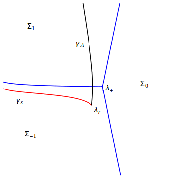
Refer to caption

Figure 8: The right half-plane, with the turning point λ+\lambda_{+} and the Stokes lines emanating from it, the Stokes sectors Σ−1,0,1\Sigma_{-1,0,1}. The further point λr\lambda_{r} and the lines γA\gamma_{A}, γS\gamma_{S} are used in the proof of Lemma 4.6.

Of the three Stokes lines emanating from λ+\lambda_{+}, one is the boundary between the Stokes sector Σ0\Sigma_{0} and Σ+1\Sigma_{+1}, another one is the boundary between the Stokes sector Σ0\Sigma_{0} and Σ−1\Sigma_{-1}, and the third one is the boundary between Σ+1\Sigma_{+1} and Σ−1\Sigma_{-1}. Notice that the region Λ+\Lambda_{+}, where the behaviour of ψ+\psi_{+} is known from Proposition 4.2, lies in the proximity of the third Stokes line, along which the solutions are oscillatory in nature33 3 Notice that the notion of Stokes sectors Σk\Sigma_{k} that we use in WKB approximation does not coincide with the notion of Stokes sectors Ωk\Omega_{k} used in Theorem 2.2. However for large λ\lambda their boundaries are asymptotic..

Therefore in order to compare ψ0\psi_{0} and ψ+\psi_{+} we need to compute the asymptotic behaviour of ψ0\psi_{0} in the union of the Stokes domains Σ1\Sigma_{1} and Σ−1\Sigma_{-1}. To this aim we express ψ0\psi_{0} as a linear combination of the solutions ψ±1​(λ)\psi_{\pm 1}(\lambda) subdominant in the Stokes domains Σ±1\Sigma_{\pm 1}. Before doing so we need to define the error function ρ±1\rho_{\pm 1} that controls the WKB estimates,

ρ±1​(λ)=infℓ∫ℓ|4​V′′​(μ)​V​(μ)−5​V′​(μ)24​V​(μ)52|​𝑑μ.\displaystyle\rho_{\pm 1}(\lambda)=\inf_{\ell}\int_{\ell}\left|\frac{4V^{\prime\prime}(\mu)V(\mu)-5V^{\prime}(\mu)^{2}}{4V(\mu)^{\frac{5}{2}}}\right|{\rm d}\mu.

Here ℓ:[0,1)→ℂ\ell\colon[0,1)\to\mathbb{C} is any path such that:

  1. (i)

    ℓ⁡(0)=λ\ell(0)=\lambda;

  2. (ii)

    ±ℜ⁡SA​(ℓ⁡(t))\pm\Re S_{A}(\ell(t)) is monotonically increasing;

  3. (iii)

    limt→1ℜ⁡SA​(ℓ⁡(t))=±∞\lim\limits_{t\to 1}\Re S_{A}(\ell(t))=\pm\infty;

see [37] for more details. We have the following lemma.

Lemma 4.5.

There exist subdominant solutions ψ~±1\widetilde{\psi}_{\pm 1} in Σ±1\Sigma_{\pm 1} of equation (4.4), uniquely characterised by the asymptotic behaviour

ψ~±1(λ;α)=VA(λ)−14ei±(SA​(λ)−π4)(1+o(1)),λ∈Σ±1and|λ|≫0.\displaystyle\widetilde{\psi}_{\pm 1}(\lambda;\alpha)=V_{A}(\lambda)^{-\frac{1}{4}}e^{i\pm(S_{A}(\lambda)-\frac{\pi}{4})}\big(1+o(1)\big),\qquad\lambda\in\Sigma_{\pm 1}\qquad\mbox{and}\qquad|\lambda|\gg 0.

Furthermore the following hold true:

  1. (i)

    Both these subdominant solutions depend holomorphically on α\alpha in DD.

  2. (ii)

    The solution ψ~0=ψ~1−ψ~−1\widetilde{\psi}_{0}=\widetilde{\psi}_{1}-\widetilde{\psi}_{-1} is subdominant in Σ0\Sigma_{0}.

  3. (iii)

    The solution ψ~0​(λ)\widetilde{\psi}_{0}(\lambda) has the following asymptotic expansion in the union of the Stokes domains Σ+1\Sigma_{+1} and Σ−1\Sigma_{-1},

    ψ~0​(λ)=VA​(λ)−14​[c1​(λ)​ei​(SA​(λ)−π4)−c−1​(λ)​e−i⁡(SA​(λ)−π4)],\displaystyle\widetilde{\psi}_{0}(\lambda)=V_{A}(\lambda)^{-\frac{1}{4}}\big[c_{1}(\lambda)e^{i(S_{A}(\lambda)-\frac{\pi}{4})}-c_{-1}(\lambda)e^{-i(S_{A}(\lambda)-\frac{\pi}{4})}\big],
    ∂ψ~0​(λ)∂λ=−VA​(λ)14​[c~1​(λ)​ei​(SA​(λ)−π4)+c~−1​(λ)​e−i⁡(SA​(λ)−π4)],\displaystyle\frac{\partial\widetilde{\psi}_{0}(\lambda)}{\partial\lambda}=-V_{A}(\lambda)^{\frac{1}{4}}\big[\tilde{c}_{1}(\lambda)e^{i(S_{A}(\lambda)-\frac{\pi}{4})}+\tilde{c}_{-1}(\lambda)e^{-i(S_{A}(\lambda)-\frac{\pi}{4}\ )}\big], (4.15)

    for some multiplicative correction terms c±1c_{\pm 1}, c~±1\tilde{c}_{\pm 1} such that |c±1​(λ)−1|=O⁡(ρ±1​(λ))|c_{\pm 1}(\lambda)-1|=O\big(\rho_{\pm 1}(\lambda)\big) and |c~±1−c±1|≤|V′​(λ)4​V​(λ)32​c±1||\tilde{c}_{\pm 1}-c_{\pm 1}|\leq\big|\frac{V^{\prime}(\lambda)}{4V(\lambda)^{\frac{3}{2}}}c_{\pm 1}\big|.

Proof.

i) For each α\alpha, the solution ψ~±1​(λ,α)\widetilde{\psi}_{\pm 1}(\lambda;\alpha) are just multiples of the subdominant solutions ψ±1\psi_{\pm 1} defined in equation (2.20). More precisely we have

ψ~±1=ψ±1×exp⁡{limλ→±i​∞(SA​(λ)−g⁡(λ,E12​α)+E2​log⁡λ)},\displaystyle\widetilde{\psi}_{\pm 1}=\psi_{\pm 1}\times\exp\left\{\lim_{\lambda\to\pm i\infty}\left(S_{A}(\lambda)-g\big(\lambda,E^{\frac{1}{2}}\alpha\big)+\frac{E}{2}\log\lambda\right)\right\},

where the ‘gg-function’ g⁡(λ,z)g(\lambda,z) was defined in (2.2). It is a standard result that the subdominant solutions (sometimes called Sibuya’s solutions) ψ±1​(α)\psi_{\pm 1}(\alpha) are entire functions of α\alpha with that given normalisation, see, e.g., [54]. Since the exponential factor is a holomorphic function of α∈D\alpha\in D, the solutions ψ~±1\widetilde{\psi}_{\pm 1} are as well.

ii) Since, by construction, ψ~1\widetilde{\psi}_{1} and ψ~−1\widetilde{\psi}_{-1} have the same dominant asymptotic behaviour in Σ0\Sigma_{0}, their difference is subdominant.

iii) The estimate (4.15) follows from the standard WKB estimates (see, e.g., [37, Appendix] or [19]).

ψ~±1​(λ)=VA​(λ)−14​c±1​(λ)​e±i⁡(SA−π4),\displaystyle\widetilde{\psi}_{\pm 1}(\lambda)=V_{A}(\lambda)^{-\frac{1}{4}}c_{\pm 1}(\lambda)e^{\pm i(S_{A}-\frac{\pi}{4})},
∂ψ~±1​(λ)∂λ=−VA​(λ)14​c~±1​(λ)​e±i⁡(SA−π4),\displaystyle\frac{\partial\widetilde{\psi}_{\pm 1}(\lambda)}{\partial\lambda}=-V_{A}(\lambda)^{\frac{1}{4}}\tilde{c}_{\pm 1}(\lambda)e^{\pm i(S_{A}-\frac{\pi}{4})},

which finishes the proof of the lemma. ∎

The error functions ρ±1\rho_{\pm 1} of the WKB approximation are estimated in the following lemma.

Lemma 4.6.

Given the hypothesis in Proposition 4.3, there exist constants E0E_{0}, CC such that, for E≥E0E\geq E_{0}, the following inequality holds

ρ±1​(λ)≤C​E−2​γ,\displaystyle\rho_{\pm 1}(\lambda)\leq CE^{-2\gamma},

for all (λ,α)∈Λ+×D(\lambda,\alpha)\in\Lambda_{+}\times D.

Proof.

The proof is in Appendix C. ∎

We can now complete the proof of Proposition 4.3. To this aim, we set ψ0​(λ,α)=E14​ψ~0​(λ,α)\psi_{0}(\lambda;\alpha)=E^{\frac{1}{4}}\widetilde{\psi}_{0}(\lambda;\alpha), where ψ~0\widetilde{\psi}_{0} is the solution studied in Lemma 4.5(ii). Due to Lemma 4.6 and Lemma 4.5(iii), there exists a CC such that

|1−c±1|≤C​E−2​γ,|1−c~±1|≤C​E−2​γ,\displaystyle|1-c_{\pm 1}|\leq CE^{-2\gamma},\qquad|1-\widetilde{c}_{\pm 1}|\leq CE^{-2\gamma},

for all (λ,α)∈Λ+×D(\lambda,\alpha)\in\Lambda_{+}\times D. In fact, the first estimate follows directly from the estimate |1−c±1|=𝒪⁡(ρ±1)|1-c_{\pm 1}|=\mathcal{O}(\rho_{\pm 1}), the second arises from the previous estimate and the fact that also V′​(λ)4​V​(λ)32=𝒪⁡(E−2​γ)\frac{V^{\prime}(\lambda)}{4V(\lambda)^{\frac{3}{2}}}=\mathcal{O}(E^{-2\gamma}) for (λ,α)∈Λ+×D(\lambda,\alpha)\in\Lambda_{+}\times D. The estimate (4.12) now follows from Lemma 4.4.

4.4 Matching and asymptotics of poles

In this subsection we complete the proof of Theorem 1.2, by comparing the asymptotic form of the solutions ψ+​(λ)\psi_{+}(\lambda) and ψ0​(λ)\psi_{0}(\lambda) of equation (4.4). These were computed in Propositions 4.2 and 4.3, on the respective domains Λ+\Lambda_{+} and Λ0\Lambda_{0}; these domains satisfy Λ+⊂Λ0\Lambda_{+}\subset\Lambda_{0}.

According to these results, on the domain Λ+\Lambda_{+} the solutions ψ0\psi_{0} and ψ+\psi_{+} share the same trigonometric form but for a generally different phase, see equations (4.7) and (4.12). The phase-difference is the following function of α\alpha,

Φ⁡(α,E)=E2​(−α​(1−α2)12+cos−1⁡(α))−(2+n)​π4\displaystyle\Phi(\alpha;E)=\frac{E}{2}\big({-}\alpha\big(1-\alpha^{2}\big)^{\frac{1}{2}}+\cos^{-1}(\alpha)\big)-\frac{(2+n)\pi}{4}
+i⁡(j​log⁡(2​(1−α2)34​E12)−12​log⁡Fn,j).\displaystyle\hphantom{\Phi(\alpha;E)=}{}+i\left(j\log\big(2\big(1-\alpha^{2}\big)^{\frac{3}{4}}E^{\frac{1}{2}}\big)-\frac{1}{2}\log F_{n,j}\right). (4.16)

Here Fn,j=Γ​[12​(1+n+j)]Γ​[12​(1+n−j)]F_{n,j}=\frac{\Gamma\big[\tfrac{1}{2}(1+n+j)\big]}{\Gamma\big[\tfrac{1}{2}(1+n-j)\big]}, as defined in (1.12). It plays a major role in our analysis. In fact, we can express the Wronskian W⁡[ψ0,ψ+]=ψ0​ψ+′−ψ0′​ψ+W[\psi_{0},\psi_{+}]=\psi_{0}\psi_{+}^{\prime}-\psi_{0}^{\prime}\psi_{+} in terms of Φ⁡(α,E)\Phi(\alpha;E).

Proposition 4.7.

Here DD is a simply connected compact subset of the vertical strip −1<ℜ⁡α<1-1<\Re\alpha<1 and ψ+​(λ)\psi_{+}(\lambda) and ψ0​(λ)\psi_{0}(\lambda) are the solutions of (4.4) studied in Proposition 4.2 and 4.3. For EE big enough we have the following decomposition of the Wronskian,

E−12​W​[ψ0,ψ+]=sin⁡(Φ⁡(α,E))+E−13​R​(α,E),\displaystyle E^{-\frac{1}{2}}W[\psi_{0},\psi_{+}]=\sin\big(\Phi(\alpha;E)\big)+E^{-\frac{1}{3}}R(\alpha,E), (4.17)

where Φ⁡(α,E)\Phi(\alpha;E) is defined in (4.16) and R⁡(α,E)R(\alpha,E) is an analytic function of α∈D\alpha\in D such that

supα∈D,E≥E0|R⁡(α,E)exp⁡(i​Φ​(α,E))|<+∞.\displaystyle\sup_{\alpha\in D,\,E\geq E_{0}}\left|\frac{R(\alpha,E)}{\exp{\big(i\Phi(\alpha,E)\big)}}\right|<+\infty.
Proof.

RR is analytic because ψ0\psi_{0}, ψ+\psi_{+} and sin⁡(Φ⁡(α,E))\sin(\Phi(\alpha;E)) are analytic in DD. The estimate is a direct consequence of Proposition 4.2 and 4.3, specialised to γ=13\gamma=\frac{1}{3}. ∎

According to the proposition above, the asymptotic distribution of the zeros of Hm,n​(α)H_{m,n}(\alpha) with nn bounded is determined by the zeros of the transcendental equation sin⁡(Φ⁡(α,E))=0\sin(\Phi(\alpha;E))=0. Equivalently

12​(α​(1−α2)12−cos−1⁡(α))+π4−E−1​i​(j​log⁡(2​(1−α2)34​E12)−12​log⁡Fn,j)=π​kE\displaystyle\frac{1}{2}\big(\alpha\big(1-\alpha^{2}\big)^{\frac{1}{2}}-\cos^{-1}(\alpha)\big)+\frac{\pi}{4}-E^{-1}i\left(j\log\big(2\big(1-\alpha^{2}\big)^{\frac{3}{4}}E^{\frac{1}{2}}\big)-\frac{1}{2}\log F_{n,j}\right)=\frac{\pi k}{E} (4.18)

for some kk, integer if mm is odd, half-integer if mm is even, whose range will be determined below.

Notice that for any compact subset of the horizontal strip −1<ℜ⁡α<1-1<{\Re}\alpha<1, equation (4.18) is just a vanishing perturbation of the equation f⁡(α)=π​kEf(\alpha)=\frac{\pi k}{E}, where f⁡(α)=12​(α​(1−α2)12−cos−1⁡(α))+π4f(\alpha)=\frac{1}{2}\big(\alpha(1-\alpha^{2})^{\frac{1}{2}}-\cos^{-1}(\alpha)\big)+\frac{\pi}{4}, because 1/f′​(α)=(1−α2)−121/f^{\prime}(\alpha)=(1-\alpha^{2})^{-\frac{1}{2}} is bounded. The equation f⁡(α)=π​kEf(\alpha)=\frac{\pi k}{E} has one and only one (and real) solution in the ’bulk’ for each |k|≤E4|k|\leq\frac{E}{4} and no solutions at all if |k|>E4|k|>\frac{E}{4}.

Since we are interested in the solutions of equation (4.18) only up to an additive error of the order E−43E^{-\frac{4}{3}}, equation (4.18) can be greatly simplified. Firstly, the imaginary part of the solutions is of order E−1​log⁡EE^{-1}\log{E} and thus we can linearise the system with respect to αI=ℑ⁡α\alpha_{I}=\Im\alpha at αI=0\alpha_{I}=0. Secondly, we can discard all terms of order E−δE^{-\delta}, δ>43\delta>\frac{4}{3} in the equation that we obtained after the linearisation with respect to αI\alpha_{I}.

These two simplifications lead to the system (1.13), whose solutions αj,k\alpha_{j,k} we described at the beginning of the present section, and to the following lemma, whose details of the proof are left to the reader.

Lemma 4.8.

For j∈Jnj\in J_{n} denote, as in Definition 1.1, by αj,k\alpha_{j,k} the unique solution of the system (1.13). Fix 0<σ<140<\sigma<\frac{1}{4}, set dR:=f−1​(π4​(1−4​σ))d_{R}:=f^{-1}\big(\frac{\pi}{4}(1-4\sigma)\big) and let dI>0d_{I}>0 be such that D0:={|ℜ⁡α|≤dR,|ℑ⁡α|≤dI}D_{0}:=\{|\Re{\alpha}|\leq d_{R},|\Im{\alpha}|\leq d_{I}\} contains all points αj,k\alpha_{j,k}, with |k|≤σ​E|k|\leq\sigma E and j∈Jnj\in J_{n}, for EE large enough, say E≥E0E\geq E_{0}.

Now, for an arbitrarily small but fixed ε\varepsilon, let D:={|ℜ⁡α|≤dR+ε,|ℑ⁡α|≤dI}D:=\{|\Re{\alpha}|\leq d_{R}+\varepsilon,|\Im{\alpha}|\leq d_{I}\}. Then there exists an E1≥E0E_{1}\geq E_{0} and a constant CC such that, for all E≥E1E\geq E_{1}, |k|≤σ​E|k|\leq\sigma E and j∈Jnj\in J_{n}, equation (4.18) has a unique solution α~j,k\tilde{\alpha}_{j,k} in DD and

|α~j,k−αj,k|≤C​E−2​log2​E.\displaystyle|\tilde{\alpha}_{j,k}-\alpha_{j,k}|\leq CE^{-2}\log^{2}E.

We have collected all the intermediate results required to prove Theorem 1.2, that we state again here.

Theorem.

Fix 0<σ<140<\sigma<\frac{1}{4}, then there exist a constant E0E_{0} and CσC_{\sigma} such that, for all E≥E0E\geq E_{0} and |k|≤σ​E|k|\leq\sigma E, the polynomial Hm,n​(z)H_{m,n}(z) has one and only one zero in each disc of the form {|z−E12αj,k|≤CσE−56}\big\{\big|z-E^{\frac{1}{2}}\alpha_{j,k}\big|\leq C_{\sigma}E^{-\frac{5}{6}}\big\}.

Proof.

We follow the proof of [38, Theorem 1] quite closely. Because of Lemma 4.8, the thesis is equivalent to: W⁡[ψ0,ψ+]​(α,E)W[\psi_{0},\psi_{+}](\alpha;E) and sin⁡(Φ⁡(α,E))\sin(\Phi(\alpha;E)) have the same number of zeros (namely one) in the disk |α−αj,k|≤C​E−43|\alpha-\alpha_{j,k}|\leq CE^{-\frac{4}{3}}.

The proof of this statement is based on Proposition 4.7 and the classical Rouché’s theorem: Let KK be a compact domain of the complex plane with simple boundary ∂K\partial K. If pp and qq are holomorphic functions, in a larger domain K′K^{\prime}, such that |q|<|p||q|<|p| on ∂K\partial K, then pp and p+qp+q have the same number of zeros – counting multiplicities – inside KK.

In our setting KK is a disc centred in αj,k\alpha_{j,k} with radius κ​E−ρ\kappa E^{-\rho} for some κ\kappa, δ\delta to be defined below, p=sin⁡(Φ⁡(α,E))p=\sin\big(\Phi(\alpha;E)\big) and q=E−12​W​[ψ0,ψ+]​(α,E)−sin⁡(Φ⁡(α,E))q=E^{-\frac{1}{2}}W[\psi_{0},\psi_{+}](\alpha;E)-\sin\big(\Phi(\alpha;E)\big).

Since σ<14\sigma<\frac{1}{4}, the αj,k\alpha_{j,k} belong to a bounded subset DD of the bulk and |αj,k2−1||\alpha_{j,k}^{2}-1| is therefore uniformly bounded from below by a positive constant. Hence, by means of a Taylor expansion estimate, for any κ>0\kappa>0, ρ>0\rho>0 there exists some numbers, cj,kc_{j,k} uniformly bounded (with the bound depending just on κ,ρ\kappa,\rho), such that ||p⁡(α)|−E1−ρ​κ​|1−αj,k2|12|≤cj,k​E1−2​ρ​κ2||p(\alpha)\big|{-}E^{1-\rho}\kappa|1-\alpha_{j,k}^{2}|^{\frac{1}{2}}\big|\leq c_{j,k}E^{1-2\rho}\kappa^{2} for any α\alpha belonging to the circle with centre αj,k\alpha_{j,k} and radius κ​E−δ\kappa E^{-\delta}.

Similarly on the union of all these circles |exp⁡(i​Φ​(α,E))||\exp{\big(i\Phi(\alpha,E)\big)}| is uniformly bounded and therefore, by Proposition 4.7 there exists a C′C^{\prime} such that, for EE large enough, |q|≤E−13​C′|q|\leq E^{-\frac{1}{3}}C^{\prime} on the union of all these circles.

Hence, for EE big enough, if ρ=43\rho=\frac{4}{3} and κ>2​C′​supj,k|1−αj,k2|−12\kappa>2C^{\prime}\sup\limits_{j,k}|1-\alpha_{j,k}^{2}|^{-\frac{1}{2}}, then |q|<|p||q|<|p| on all the circles with centre αj,k\alpha_{j,k} and radius κ​E−ρ\kappa E^{-\rho}. This concludes the proof. ∎

4.5 Proof of Theorem 1.3.

Recall that in stating and proving Theorem 1.2 and all necessary preparatory lemmas and propositions, we worked with a compact subset DD of the α\alpha-plane not containing the points α=±1\alpha=\pm 1. This is because all estimates involved break down at those two points.

However, we can improve our results without modifying the procedures if we let DED_{E} vary with EE and approach the points ±1\pm 1 slowly enough. To this aim we fix δ>13\delta>\frac{1}{3} and we assume that the distance of DED_{E} from α=±1\alpha=\pm 1 is greater or equal to a constant times E−1+δE^{-1+\delta}.

Indeed, we can prove Theorem 1.3 that we state again here for convenience.

Theorem.

Fix 13<δ≤1\frac{1}{3}<\delta\leq 1 and s>0s>0. There exist a constant E0E_{0} and a constant CsC_{s} such that, if E≥E0E\geq E_{0}, then for all |k|≤(14−s​E3​−1+δ2)​E|k|\leq\big(\frac{1}{4}-sE^{3\frac{-1+\delta}{2}}\big)E, the polynomial Hm,n​(z)H_{m,n}(z) has one and only one zero in each disc of the form |z−E12​αj,k|≤Cs​E−δ+16\big|z-E^{\frac{1}{2}}\alpha_{j,k}\big|\leq C_{s}E^{-\delta+\frac{1}{6}}.

Proof.

We assume that α∈DE\alpha\in D_{E}, where DED_{E} is a compact simply connected domain whose distance to the points α=±1\alpha=\pm 1 is bigger or equal than a constant times E1−δE^{1-\delta}. In other words, there exists a c>0c>0 such that supα∈DE|(1−α2)−1|≤c​Eδ−1\sup\limits_{\alpha\in D_{E}}|(1-\alpha^{2})^{-1}|\leq cE^{\delta-1}.

It turns out that the statement of Propositions 4.1, 4.2, 4.3 and 4.7 holds true if we appropriately modify the error bounds.

Below, we list the necessary modification, whose verification is straightforward.

  • (i)

    In Proposition 4.1(ii). The equation (4.7) must be modified as follows. For j∈Jnj\in J_{n}, the branch βj​(α)\beta_{j}(\alpha) has the following asymptotic expansion

    OPENβj​(α,E)=j​i​(1−α2)12​(1+E1−3​δ2​rj​(α,E))),\displaystyle\beta_{j}(\alpha,E)=ji\big(1-\alpha^{2}\big)^{\frac{1}{2}}\big(1+E^{\frac{1-3\delta}{2}}r_{j}(\alpha,E))\big),

    where rj​(α,E)r_{j}(\alpha,E) is a bounded function on DE×[E0,∞)D_{E}\times[E_{0},\infty).

  • (ii)

    Proposition 4.2, having fixed γ=3​δ−16\gamma=\frac{3\delta-1}{6}, holds true if the error terms in the estimate (4.7) are modified as follows

    |ψ+​(λ)−Σ⁡(λ,j,φ,χ)|≤C​E−3​δ−16,\displaystyle|\psi_{+}(\lambda)-\Sigma(\lambda;j,\varphi,\chi\big)|\leq CE^{-\frac{3\delta-1}{6}},
    |E−12​ψ+′​(λ)+Σ⁡(λ,j,φ+12​π,χ)|≤C​E−3​δ−16.\displaystyle\big|E^{-\frac{1}{2}}\psi_{+}^{\prime}(\lambda)+\Sigma\big(\lambda;j,\varphi+\tfrac{1}{2}\pi,\chi\big)\big|\leq CE^{-\frac{3\delta-1}{6}}.
  • (iii)

    Proposition 4.3, having fixed γ=3​δ−16\gamma=\frac{3\delta-1}{6}, holds true if the error bound in equations (4.7) is modified as follows

    |ψ0​(λ,α)−Σ⁡(λ,j,φ′,χ′)|≤C​E−3​δ−16​(|Σ⁡(λ,j,φ′,χ′)|+|Σ⁡(λ,j,φ′+12​π,χ′)|),\displaystyle\big|\psi_{0}(\lambda;\alpha)-\Sigma(\lambda;j,\varphi^{\prime},\chi^{\prime})\big|\leq CE^{-\frac{3\delta-1}{6}}\big(|\Sigma(\lambda;j,\varphi^{\prime},\chi^{\prime})|+\big|\Sigma\big(\lambda;j,\varphi^{\prime}+\tfrac{1}{2}\pi,\chi^{\prime}\big)\big|\big),
    |E−12​∂ψ0​(λ,α)∂λ+Σ⁡(λ,j,φ′+12​π,χ′)|\displaystyle\left|E^{-\frac{1}{2}}\frac{\partial\psi_{0}(\lambda;\alpha)}{\partial\lambda}+\Sigma\big(\lambda;j,\varphi^{\prime}+\tfrac{1}{2}\pi,\chi^{\prime}\big)\right|
    ≤C​E−3​δ−16​(|Σ⁡(λ,j,φ′,χ′)|+|Σ⁡(λ,j,φ′+12​π,χ′)|).\displaystyle\qquad{}\leq CE^{-\frac{3\delta-1}{6}}\big(|\Sigma(\lambda;j,\varphi^{\prime},\chi^{\prime})|+\big|\Sigma\big(\lambda;j,\varphi^{\prime}+\tfrac{1}{2}\pi,\chi^{\prime}\big)\big|\big).
  • (iv)

    Proposition 4.7 holds true if the error bound in equation (4.17) is modified as follows

    E−12​W​[ψ0,ψ+]=sin⁡(Φ⁡(α,E))+E−3​δ−16​R​(α,E).\displaystyle E^{-\frac{1}{2}}W[\psi_{0},\psi_{+}]=\sin\big(\Phi(\alpha;E)\big)+E^{-\frac{3\delta-1}{6}}R(\alpha,E).
  • (v)

    Finally the estimate of Lemma 4.8 about the distance among solutions α~j,k\tilde{\alpha}_{j,k} of equation (4.18) and the points αj,k\alpha_{j,k} is modified as follows: For kk in the range of the present Theorem, there exists a constant CC depending on ss such that

    |α~j,k−αj,k|≤C​E−2​δ​log2​E.\displaystyle|\tilde{\alpha}_{j,k}-\alpha_{j,k}|\leq CE^{-2\delta}\log^{2}E.

We notice that as ℜ⁡α→1−\Re\alpha\to 1^{-}, we have f⁡(α)=2323​(1−α)32+𝒪⁡((1−α)52)f(\alpha)=\frac{2^{\frac{3}{2}}}{3}(1-\alpha)^{\frac{3}{2}}+\mathcal{O}\big((1-\alpha)^{\frac{5}{2}}\big) (and a similar behaviour for ℜ⁡α→−1+\Re\alpha\to-1^{+}). Therefore, we can appropriately choose a c>0c>0 such that all solutions of the system (1.13), with kk in the given range, belong to the strip −1+c​E−1+δ≤ℜ⁡α≤1−c​E−1+δ-1+cE^{-1+\delta}\leq\Re\alpha\leq 1-cE^{-1+\delta}.

The proof can then be continued following the very same steps of the proof of Theorem 1.2; we prove that Hm,n​(E12​α)H_{m,n}\big(E^{\frac{1}{2}}\alpha\big) has one and only one zero in each disc of the form |α−αj,k|≤Cs​E−5+3​δ6|\alpha-\alpha_{j,k}|\leq C_{s}E^{-\frac{5+3\delta}{6}}. Indeed we again set p=sin⁡(Φ⁡(α,E))p=\sin(\Phi(\alpha;E)) and q=E−12​W​[ψ0,ψ+]​(α,E)−sin⁡(Φ⁡(α,E))q=E^{-\frac{1}{2}}W[\psi_{0},\psi_{+}](\alpha;E)-\sin(\Phi(\alpha;E)).

We fix some κ,ρ>0\kappa,\rho>0 and estimate the value of |p⁡(α)||p(\alpha)| for α\alpha belonging to the circle with centre αj,k\alpha_{j,k} and radius κ​E−ρ\kappa E^{-\rho}. By means of a Taylor series estimate, and taking in account that |1−α2|≥c​E−1+δ|1-\alpha^{2}|\geq cE^{-1+\delta} and δ>13\delta>\frac{1}{3}, we obtain the following lower bound of pp on the aforementioned circles: if EE is big enough, there exists a c′c^{\prime} (depending on cc) such that, on the union of all these circles, |p⁡(α)|≥c′​E1+δ2−ρ|p(\alpha)|\geq c^{\prime}E^{\frac{1+\delta}{2}-\rho} provided ρ>1−δ\rho>1-\delta. Due to the above modification of Proposition 4.7, there exists a c′′c^{\prime\prime} (depending on cc) such that on the union of the circle |q⁡(α)|≤c′′​E−3​δ+16|q(\alpha)|\leq c^{\prime\prime}E^{-\frac{3\delta+1}{6}}.

Therefore as long as 1−δ<ρ≤δ+131-\delta<\rho\leq\delta+\frac{1}{3}, and EE is big enough, we can find a κ\kappa such that |q|<|p||q|<|p| on the aforementioned circle. The thesis then follows from Rouché’s theorem. ∎

4.6 Edge asymptotics

In this last section of the paper we briefly discuss the edge asymptotic in the regime nn bounded and E=2​m+n→∞E=2m+n\to\infty. We anticipate below some preliminary results about the edge-asymptotic and we postpone more details and full proofs to a further publication.

Recall that the proof of Theorem 1.3 breaks down when 1−α2=𝒪⁡(E−23)1-\alpha^{2}=\mathcal{O}\big(E^{-\frac{2}{3}}\big), because in that regime the error of our asymptotic method is of the same order as the distance between the roots, as depicted in Fig. 9.

Refer to caption Refer to caption
m=16m=16 m=144m=144
Figure 9: Rescaled roots of Hm,5H_{m,5} in upper right corner. In blue numerically exact location, in red the asymptotic approximation αj,k\alpha_{j,k}, encircled by a circle of radius Cs​E−23C_{s}E^{-\frac{2}{3}}, with Cs=16C_{s}=\frac{1}{6}, for the range m+12−k∈{0,1,2}\frac{m+1}{2}-k\in\{0,1,2\}, j∈{0,2,4}j\in\{0,2,4\}. Even though the approximation by αj,k\alpha_{j,k} still look reasonably good, it does not give the dominant term in the asymptotic expansion of extreme roots. This is reflected in the fact that the absolute error of Theorem 1.3, if extrapolated at the value δ=13\delta=\frac{1}{3}, is of the same order of the distance between roots, namely E−23E^{-\frac{2}{3}} .

However, our procedures can be adapted appropriately to study the limit 1−α2=𝒪⁡(E−23)1-\alpha^{2}=\mathcal{O}\big(E^{-\frac{2}{3}}\big). Without losing generality we restrict our discussion to the case α→1\alpha\to 1.

As a first step we make the Ansatz 1−α=κ​E−231-\alpha=\kappa E^{-\frac{2}{3}} and look for κ\kappa of order E0E^{0} that solves the inverse monodromy problem for Hermite I rational solutions of PIV{\rm P}_{\rm IV}, equation (4.1). Upon inserting the Ansatz in equation (4.1), redefining the unknown β→E13​β\beta\to E^{\frac{1}{3}}\beta, and discarding lower order contributions, equation (4.1) reads

ψ′′​(λ)=Vκ​(λ,κ,β,E,n)​ψ​(λ),\displaystyle\psi^{\prime\prime}(\lambda)=V_{\kappa}(\lambda;\kappa,\beta,E,n)\psi(\lambda),
Vκ​(λ)=λ2+2​E12​λ−2​κ​E13−E16​βλ+n2−14​λ2.\displaystyle V_{\kappa}(\lambda)=\lambda^{2}+2E^{\frac{1}{2}}\lambda-2\kappa E^{\frac{1}{3}}-\frac{E^{\frac{1}{6}}\beta}{\lambda}+\frac{n^{2}-1}{4\lambda^{2}}.

We look for (κ,β)(\kappa,\beta) such that no-logarithm and quantisation conditions hold.

No-logarithm in the edge. Reasoning as in Proposition 4.1, we can express the unknown β\beta as an n-valued function of the unknown κ\kappa. To this aim, we apply the change of coordinates ν=E−16​λ\nu=E^{-\frac{1}{6}}\lambda. The resulting equation reads

ψ′′=(E−23​ν2+2​ν−2​κ−βν+n2−14​ν2)​ψ.\displaystyle\psi^{\prime\prime}=\left(E^{-\frac{2}{3}}\nu^{2}+2\nu-2\kappa-\frac{\beta}{\nu}+\frac{n^{2}-1}{4\nu^{2}}\right)\psi.

Therefore β=βj​(κ)​(1+𝒪⁡(E−23))\beta=\beta_{j}(\kappa)\big(1+\mathcal{O}(E^{-\frac{2}{3}})\big) where βj​(κ)\beta_{j}(\kappa), j∈Jnj\in J_{n} is one of the nn solutions of the no-logarithm condition for the equation

ψ′′=(2​ν−2​κ−βν+n2−14​ν2)​ψ.\displaystyle\psi^{\prime\prime}=\left(2\nu-2\kappa-\frac{\beta}{\nu}+\frac{n^{2}-1}{4\nu^{2}}\right)\psi. (4.19)

The above equation does not belong to the any standard class of linear special functions listed in [50] or [16]. In particular, the solution of the no-logarithm condition for the latter equation does not seem to have a simple factorisation. For the sake of the present discussion we assume that for ℜ⁡κ>0\Re\kappa>0, the functions βj​(κ)\beta_{j}(\kappa) are all distinct as in the case of the Whittaker equation.

Airy-like model near the origin. Applying again the change of variable ν=E−16​λ\nu=E^{-\frac{1}{6}}\lambda, and reasoning as in Proposition 4.2, we deduce that the solution ψ+\psi_{+} is asymptotic to the solution u+​(ν)u_{+}(\nu), subdominant at λ=0\lambda=0, of the equation

u′′​(ν)=(2​ν−2​κ−βj​(κ)ν+n2−14​ν2)​u​(ν).\displaystyle u^{\prime\prime}(\nu)=\left(2\nu-2\kappa-\frac{\beta_{j}(\kappa)}{\nu}+\frac{n^{2}-1}{4\nu^{2}}\right)u(\nu). (4.20)

The latter equation is an Airy equation with a centrifugal term. The solution u+​(ν)u_{+}(\nu) is thus for generic values of κ\kappa dominant at +∞+\infty. However, we say that κ\kappa is an eigenvalue of equation (4.20) if u+​(ν)u_{+}(\nu) is subdominant at +∞+\infty.

Matching. The asymptotic analysis of the solution ψ0\psi_{0} simplifies in this regime. In fact, in the large EE limit, the turning points λ+\lambda_{+} and λ−\lambda_{-} coalesce with the Fuchsian singularity λ=0\lambda=0. Therefore the standard approximation ψ0∼VA−14​e−SA\psi_{0}\sim V_{A}^{-\frac{1}{4}}e^{-S_{A}} is valid in a region close to λ=0\lambda=0, where the approximation of ψ+\psi_{+} by u+u_{+} is also valid. Finally, reasoning as in Proposition 4.7, we deduce that, asymptotically, the solutions ψ+\psi_{+} and ψ0\psi_{0} are proportional if and only if κ\kappa is one of the eigenvalue of (4.20).44 4 Remarkably a slightly simpler version of this problem was shown to model the growth-rate distribution of E. Coli, see [10] by one of the authors.

Extremal asymptotic. We have therefore arrived at a (preliminary) description for the edge asymptotic for roots with extreme real part, without entering into the details of estimating the error of the approximation: Let (κ,β)(\kappa,\beta) be such that the Airy-like equation (4.19) satisfies the no-logarithm condition and the quantisation condition limν→+∞u+​(ν)=0\lim\limits_{\nu\to+\infty}u_{+}(\nu)=0. If EE is big enough, there exists a root of the generalised Hermite polynomial Hm,n​(α)H_{m,n}(\alpha) with the asymptotic behaviour 1−α=κ​E−23+o⁡(E−23)1-\alpha=\kappa E^{-\frac{2}{3}}+o(E^{-\frac{2}{3}}).

Remark 4.9.

In the case n=1n=1, the above description coincides with the well known edge-asymptotic for roots of the Hermite polynomial [16]. Indeed, in the case n=1n=1, the only solution of the no-logarithm condition is β=0\beta=0: the equation (4.19) reduces to the standard Airy equation with potential 2​λ−2​κ2\lambda-2\kappa and u+u_{+} is the solution of the Airy equation that vanishes at λ=0\lambda=0. Therefore the eigenvalues equal κn=−2−13​εn,n≥1\kappa_{n}=-2^{-\frac{1}{3}}\varepsilon_{n},n\geq 1 where εn\varepsilon_{n} is the nn-th zero of the Airy function on the imaginary axis.

5 Concluding remarks

All singularities of Painlevé IV rationals can be expressed in terms of zeros of generalised Hermite Hm,nH_{m,n} and Okamoto polynomials Qm,nQ_{m,n}. We have characterised those zeros by means of the inverse monodromy problem for an anharmonic oscillator of degree two. We have shown that these oscillators in turn characterise three special classes of infinitely sheeted coverings of the sphere. In the case of generalised Hermite polynomials we have also explicitly computed the monodromy representation of such coverings by means of line complexes; as a by-product we obtained the number of real roots. Finally we have computed the asymptotic distribution in the bulk of zeros of generalised Hermite polynomials in the regime m≫0m\gg 0 and nn fixed; we have also presented some preliminary results about the edge asymptotics.

Many questions about rational solutions of Painlevé IV remain open and we plan to address some of them by means of the methods developed in the present paper. These include, in the case of generalised Hermite polynomials, a precise description of zeros in the edge – in particular the cross-over between the bulk and the edge behaviour described by the large κ\kappa limit of equation (4.20) – and the asymptotic distribution of zeros in the more general regime r:=m/n∈(0,1]r:=m/n\in(0,1] fixed and both m,n→∞m,n\rightarrow\infty. The latter is in principle a straightforward extension of our results, even though the error analysis presents some new analytical challenges.

The real testing ground of our methods is the analysis of Okamoto polynomials. On the theoretical side, we have yet to find a combinatorial classification of line complexes of the functions in the class F3nF_{3}^{n} discussed in Section 3. Such a classification would lead, along the lines of Corollary 3.5, to compute the number of real zeros. We also plan to tackle the asymptotic analysis of the distribution of zeros of generalised Okamoto polynomials, but at this stage it is uncertain whether our methods allows to deal with the greater complexity of these polynomials.

Appendix A Generalised Hermite and Okamoto polynomials

The generalised Hermite polynomials Hm,n​(z)H_{m,n}(z), where m,n∈ℕm,n\in\mathbb{N}, are recursively defined by

2​m​Hm+1,n​Hm−1,n=Hm,n​Hm,n′′−(Hm,n′)2+2​m​Hm,n2,\displaystyle 2mH_{m+1,n}H_{m-1,n}=H_{m,n}H_{m,n}^{\prime\prime}-(H_{m,n}^{\prime})^{2}+2mH_{m,n}^{2},
2​n​Hm,n+1​Hm,n−1=−Hm,n​Hm,n′′+(Hm,n′)2+2​n​Hm,n2,\displaystyle 2nH_{m,n+1}H_{m,n-1}=-H_{m,n}H_{m,n}^{\prime\prime}+(H_{m,n}^{\prime})^{2}+2nH_{m,n}^{2},

with H0,0=H1,0=H0,1=1H_{0,0}=H_{1,0}=H_{0,1}=1 and H1,1=2​zH_{1,1}=2z. Specialising to n=1n=1, we obtain the classical mm-th Hermite polynomial, that is,

Hm,1​(z)=(−1)m​ez2​∂m∂zm​[e−z2].\displaystyle H_{m,1}(z)=(-1)^{m}e^{z^{2}}\frac{\partial^{m}}{\partial z^{m}}\big[e^{-z^{2}}\big].

Similarly the generalised Okamoto polynomials Qm,nQ_{m,n}, where m,n∈ℤm,n\in\mathbb{Z}, are defined via the recursion

Qm+1,n​Qm−1,n=92​(Qm,n​Qm,n′′−(Qm,n′)2)+(2​z2+3​(2​m+n−1))​Qm,n2,\displaystyle Q_{m+1,n}Q_{m-1,n}=\tfrac{9}{2}\big(Q_{m,n}Q_{m,n}^{\prime\prime}-(Q_{m,n}^{\prime})^{2}\big)+\big(2z^{2}+3(2m+n-1)\big)Q_{m,n}^{2},
Qm,n+1​Qm,n−1=92​(Qm,n​Qm,n′′+(Qm,n′)2)+(2​z2+3​(1−m−2​n))​Qm,n2,\displaystyle Q_{m,n+1}Q_{m,n-1}=\tfrac{9}{2}\big(Q_{m,n}Q_{m,n}^{\prime\prime}+(Q_{m,n}^{\prime})^{2}\big)+\big(2z^{2}+3(1-m-2n)\big)Q_{m,n}^{2},

with Q0,0=Q1,0=Q0,1=1Q_{0,0}=Q_{1,0}=Q_{0,1}=1 and Q1,1=2​zQ_{1,1}=\sqrt{2}z. The polynomials Qm,0Q_{m,0} and Qm,1Q_{m,1} with m∈ℤm\in\mathbb{Z}, were originally introduced by Okamoto [49], to describe the subcases of (1.7) where θ0∈{±16,±13}\theta_{0}\in\big\{\pm\frac{1}{6},\pm\frac{1}{3}\big\}.

Proposition A.1.

For m,n∈ℕm,n\in\mathbb{N}, the polynomial Hm,nH_{m,n} has only simple roots and none common with Hm+1,nH_{m+1,n}, Hm,n+1H_{m,n+1} and Hm−1,n+1H_{m-1,n+1}. Furthermore Hm,n​(12​z)H_{m,n}\big(\frac{1}{2}z\big) is monic of degree m​nmn with integer coefficients and we have the symmetry

Hm,n​(i​z)=im​n​Hn,m​(z).\displaystyle H_{m,n}(iz)=i^{mn}H_{n,m}(z).

For m,n∈ℤm,n\in\mathbb{Z}, the polynomial Qm,nQ_{m,n} has only simple roots and none common with Qm+1,nQ_{m+1,n}, Qm,n+1Q_{m,n+1} and Qm−1,n+1Q_{m-1,n+1}. Furthermore Qm,n​(12​z)Q_{m,n}\big(\frac{1}{\sqrt{2}}z\big) is monic of degree dm,n=m2+n2+m​n−m−nd_{m,n}=m^{2}+n^{2}+mn-m-n with integer coefficients and we have the symmetries

Qm,n​(i​z)=idm,n​Qn,m​(z),Qm,n​(z)=Q−m−n+1,m​(z).\displaystyle Q_{m,n}(iz)=i^{d_{m,n}}Q_{n,m}(z),\qquad Q_{m,n}(z)=Q_{-m-n+1,m}(z).
Proof.

See Noumi and Yamada [46]. ∎

Appendix B Bäcklund transformations

Okamoto [49] first uncovered that PIV{\rm P}_{\rm IV} enjoys the action of the affine Weyl group A1(1)A_{1}^{(1)} by means of Bäcklund transformations on its solutions, see also Noumi and Yamada [46]. In this study we only require the including translations, generated by

ℛ1:\displaystyle\mathcal{R}_{1}\colon\quad ω(1)=(ω′+4​θ0)2+8​(θ∞−θ0)​ω2−ω2​(ω+2​z)22​ω​(ω2+2​z​ω−ω′−4​θ0),\displaystyle\omega^{(1)}=\frac{(\omega^{\prime}+4\theta_{0})^{2}+8(\theta_{\infty}-\theta_{0})\omega^{2}-\omega^{2}(\omega+2z)^{2}}{2\omega(\omega^{2}+2z\omega-\omega^{\prime}-4\theta_{0})},
ℛ2:\displaystyle\mathcal{R}_{2}\colon\quad ω(2)=(ω′−4​θ0)2+8​(θ∞−1−θ0)​ω2−ω2​(ω+2​z)22​ω​(ω2+2​z​ω+ω′−4​θ0),\displaystyle\omega^{(2)}=\frac{(\omega^{\prime}-4\theta_{0})^{2}+8(\theta_{\infty}-1-\theta_{0})\omega^{2}-\omega^{2}(\omega+2z)^{2}}{2\omega(\omega^{2}+2z\omega+\omega^{\prime}-4\theta_{0})},
ℛ3:\displaystyle\mathcal{R}_{3}\colon\quad ω(3)=(ω′−4​θ0)2+8​(θ∞+θ0)​ω2−ω2​(ω+2​z)22​ω​(ω2+2​z​ω−ω′+4​θ0),\displaystyle\omega^{(3)}=\frac{(\omega^{\prime}-4\theta_{0})^{2}+8(\theta_{\infty}+\theta_{0})\omega^{2}-\omega^{2}(\omega+2z)^{2}}{2\omega(\omega^{2}+2z\omega-\omega^{\prime}+4\theta_{0})},
ℛ4:\displaystyle\mathcal{R}_{4}\colon\quad ω(4)=(ω′+4​θ0)2+8​(θ∞−1+θ0)​ω2−ω2​(ω+2​z)22​ω​(ω2+2​z​ω+ω′+4​θ0),\displaystyle\omega^{(4)}=\frac{(\omega^{\prime}+4\theta_{0})^{2}+8(\theta_{\infty}-1+\theta_{0})\omega^{2}-\omega^{2}(\omega+2z)^{2}}{2\omega(\omega^{2}+2z\omega+\omega^{\prime}+4\theta_{0})}, (B.1)

where the complex parameters are transformed correspondingly as

θ0(1)=θ0−12,\displaystyle\theta_{0}^{(1)}=\theta_{0}-\tfrac{1}{2},\qquad θ0(2)=θ0+12,\displaystyle\theta_{0}^{(2)}=\theta_{0}+\tfrac{1}{2},\qquad θ0(3)=θ0+12,\displaystyle\theta_{0}^{(3)}=\theta_{0}+\tfrac{1}{2},\qquad θ0(4)=θ0−12,\displaystyle\theta_{0}^{(4)}=\theta_{0}-\tfrac{1}{2},
θ∞(1)=θ∞+12,\displaystyle\theta_{\infty}^{(1)}=\theta_{\infty}+\tfrac{1}{2},\qquad θ∞(2)=θ∞−12,\displaystyle\theta_{\infty}^{(2)}=\theta_{\infty}-\tfrac{1}{2},\qquad θ∞(3)=θ∞+12,\displaystyle\theta_{\infty}^{(3)}=\theta_{\infty}+\tfrac{1}{2},\qquad θ∞(4)=θ∞−12.\displaystyle\theta_{\infty}^{(4)}=\theta_{\infty}-\tfrac{1}{2}.

It is these Bäcklund transformations, which can be extended to Schlesinger transformations of the associated linear system (2.6), as shown by Fokas et al. [24]. Note that the following identities hold true

ℛ1​ℛ2=ℐ,ℛ3​ℛ4=ℐ,ℛ1​ℛ3=ℛ3​ℛ1,\displaystyle\mathcal{R}_{1}\mathcal{R}_{2}=\mathcal{I},\qquad\mathcal{R}_{3}\mathcal{R}_{4}=\mathcal{I},\qquad\mathcal{R}_{1}\mathcal{R}_{3}=\mathcal{R}_{3}\mathcal{R}_{1},

where ℐ\mathcal{I} denotes the identity.

Appendix C WKB Computations

Proof of Lemma 4.4.

After the change of variable ν=E−12​μ+α\nu=E^{-\frac{1}{2}}\mu+\alpha, the integral reads

SA​(λ)=E​∫E−12​λ+αE−12​λ++α1−ν2+j​i​(1−α2)12E⁡(ν−α)−n2−14​E2​(ν−α)2​𝑑ν,\displaystyle S_{A}(\lambda)=E\int^{E^{-\frac{1}{2}}\lambda_{+}+\alpha}_{E^{-\frac{1}{2}}\lambda+\alpha}\sqrt{1-\nu^{2}+\frac{ji(1-\alpha^{2})^{\frac{1}{2}}}{E(\nu-\alpha)}-\frac{n^{2}-1}{4E^{2}(\nu-\alpha)^{2}}}{\rm d}\nu,

where, by equation (4.13), we have E−12​λ++α=1+j​i2​(1−α)​E−1+𝒪⁡(E−2)E^{-\frac{1}{2}}\lambda_{+}+\alpha=1+\frac{ji}{2(1-\alpha)}E^{-1}+\mathcal{O}(E^{-2}). We introduce a fixed but arbitrarily small ε>0\varepsilon>0 and shift the upper integration limit to get

SA​(λ)=E​∫E−12​λ+α1+i​E−1+ε1−ν2+j​i​(1−α2)12E⁡(ν−α)−n2−14​E2​(ν−α)2​𝑑ν+𝒪⁡(E−1−3​ε2).\displaystyle S_{A}(\lambda)=E\int^{1+iE^{-1+\varepsilon}}_{E^{-\frac{1}{2}}\lambda+\alpha}\sqrt{1-\nu^{2}+\frac{ji(1-\alpha^{2})^{\frac{1}{2}}}{E(\nu-\alpha)}-\frac{n^{2}-1}{4E^{2}(\nu-\alpha)^{2}}}{\rm d}\nu+\mathcal{O}\big(E^{-\frac{1-3\varepsilon}{2}}\big).

Next, expanding the integrand about E=∞E=\infty, gives

SA​(λ)=∫E−12​λ+α1+i​E−1+ε(E​1−ν2+12​j​i​(1−α2)12(ν−α)​(1−ν2)12)​𝑑ν\displaystyle S_{A}(\lambda)=\int^{1+iE^{-1+\varepsilon}}_{E^{-\frac{1}{2}}\lambda+\alpha}\left(E\sqrt{1-\nu^{2}}+\tfrac{1}{2}ji\frac{(1-\alpha^{2})^{\frac{1}{2}}}{(\nu-\alpha)(1-\nu^{2})^{\frac{1}{2}}}\right){\rm d}\nu
+∫E−12​λ+α1+i​E−1+ε∑k≥2E−k+1ck(ν−α)k​(1−ν2)k−12dν+𝒪(E−1−3​ε2),\displaystyle\hphantom{S_{A}(\lambda)=}{}+\int^{1+iE^{-1+\varepsilon}}_{E^{-\frac{1}{2}}\lambda+\alpha}\sum_{k\geq 2}E^{-k+1}\frac{c_{k}}{(\nu-\alpha)^{k}(1-\nu^{2})^{k-\frac{1}{2}}}{\rm d}\nu+\mathcal{O}\big(E^{-\frac{1-3\varepsilon}{2}}\big), (C.1)

where the series ∑ck​wk\sum c_{k}w^{k} has positive radius of convergence r0r_{0}.

In the first line, discarding again an error 𝒪⁡(E−1−3​ε2)\mathcal{O}\big(E^{-\frac{1-3\varepsilon}{2}}\big), the upper integration limit can be replaced by 11, and the remaining integral can be written explicitly in terms of elementary functions. Indeed, the integral of the first term of the first line equals

14​E​(−2​(α+λ​E−12)​1−(α+λ​E−12)2−2​arcsin⁡(α+λ​E−12)+π),\displaystyle\tfrac{1}{4}E\big({-}2\big(\alpha+\lambda E^{-\frac{1}{2}}\big)\sqrt{1-\big(\alpha+\lambda E^{-\frac{1}{2}}\big)^{2}}-2\arcsin\big(\alpha+\lambda E^{-\frac{1}{2}}\big)+\pi\big),

which in the limit λ≍E−12+γ\lambda\asymp E^{-\frac{1}{2}+\gamma} yields

12​E​(−α​(1−α2)12+arccos⁡α)−E12​(1−α2)12​λ+𝒪⁡(E−1+2​γ).\displaystyle\tfrac{1}{2}E\big({-}\alpha\big(1-\alpha^{2}\big)^{\frac{1}{2}}+\arccos{\alpha}\big)-E^{\frac{1}{2}}\big(1-\alpha^{2}\big)^{\frac{1}{2}}\lambda+\mathcal{O}\big(E^{-1+2\gamma}\big).

The second term of the first line of (C.1) is equal to

12​j​i​(−log⁡λ+12​log⁡E+log⁡[(1−α2)​(1−(α+E−12​λ)2)−α⁡(α+E−12​λ)+1]),\displaystyle\tfrac{1}{2}ji\Big({-}\log\lambda+\tfrac{1}{2}\log E+\log\Big[\sqrt{\big(1-\alpha^{2}\big)\big(1-\big(\alpha+E^{-\frac{1}{2}}\lambda\big)^{2}\big)}-\alpha\big(\alpha+E^{-\frac{1}{2}}\lambda\big)+1\Big]\Big),

and in the limit λ≍E−12+γ\lambda\asymp E^{-\frac{1}{2}+\gamma} yields

12​j​i​(−log⁡λ+log⁡E12+log⁡2​(1−α2))+𝒪⁡(E−1+γ).\displaystyle\tfrac{1}{2}ji\big({-}\log\lambda+\log E^{\frac{1}{2}}+\log 2(1-\alpha^{2})\big)+\mathcal{O}\big(E^{-1+\gamma}\big).

To conclude the proof, we show that for λ≍E−12+γ\lambda\asymp E^{-\frac{1}{2}+\gamma} the second line of (C.1) is of order E−γE^{-\gamma}, if ε\varepsilon is sufficiently small. We therefore fix s∈ℂs\in\mathbb{C}, ℜ⁡s>0\Re s>0 and let λ=s​E−12+γ\lambda=sE^{-\frac{1}{2}+\gamma} (γ≥0\gamma\geq 0).

Since the contribution of the endpoints is different, we split the integration contour in two, namely ∫E−12​λ+α1+α2\int_{E^{-\frac{1}{2}}\lambda+\alpha}^{\frac{1+\alpha}{2}} and ∫1+α21+i​E−1+ε\int_{\frac{1+\alpha}{2}}^{1+iE^{-1+\varepsilon}}.

Along the first sub-contour, after the change of variable ρ=E1−γ​(ν−α)\rho=E^{1-\gamma}(\nu-\alpha), the integrand becomes

∫sE1−γ​(1−α2)∑k≥2E−γ⁡(k−1)​ck​ρ−k​(1−(Eγ−1​ρ+α)2)−k+12​𝑑ρ.\displaystyle\int_{s}^{E^{1-\gamma}(1-\frac{\alpha}{2})}\sum_{k\geq 2}E^{-\gamma(k-1)}c_{k}\rho^{-k}\big(1-\big(E^{\gamma-1}\rho+\alpha\big)^{2}\big)^{-k+\frac{1}{2}}{\rm d}\rho.

Estimating (1−(Eγ−1​ρ+α)2)−k+12(1-(E^{\gamma-1}\rho+\alpha)^{2})^{-k+\frac{1}{2}} with its supremum, the radius of convergence of the series is easily estimated to be at least Eγ​(1−α2)​s​r0E^{\gamma}(1-\alpha^{2})sr_{0}. Therefore, for EE large enough, the integrand is seen to converge uniformly and the dominant contribution is 𝒪⁡(E−γ)\mathcal{O}(E^{-\gamma}).

Similar considerations, along the second sub-contour, lead to a dominant contribution of order 𝒪⁡(E−1+ε2)\mathcal{O}(E^{-\frac{1+\varepsilon}{2}}). ∎

Proof of Lemma 4.6.

We prove the lemma for ρ1\rho_{1}. An analogue proof is valid for the case ρ−1\rho_{-1}.

For any potential VV, we define the function R⁡(V,λ)=4​V′′​(λ)​V​(λ)−5​V′​(λ)2V​(λ)52R(V,\lambda)=\frac{4V^{\prime\prime}(\lambda)V(\lambda)-5V^{\prime}(\lambda)^{2}}{V(\lambda)^{\frac{5}{2}}}.

By definition ρ1≤∫ℓ|R⁡(VA,μ)​𝑑μ|\rho_{1}\leq\int_{\ell}|R(V_{A},\mu){\rm d}\mu| where the oriented integration contour ℓ\ell is such that along it the real part of the phase function, ℜ⁡SA\Re{S_{A}}, is not decreasing and tends to +∞+\infty

To this aim, we fix some 0<r<1−ℜ⁡α0<r<1-\Re\alpha and define the following integration contour

∫λ,γSλr|R⁡(VA,μ)|𝑑μ+∫λr,γA∞|R⁡(VA,μ)|​𝑑μ,\displaystyle\int_{\lambda,\gamma_{S}}^{\lambda_{r}}|R(V_{A},\mu)|{\rm d}\mu+\int_{\lambda_{r},\gamma_{A}}^{\infty}|R(V_{A},\mu)|{\rm d}\mu,

where λr\lambda_{r} is the intercept with real part E12​rE^{\frac{1}{2}}r of the Stokes line γS\gamma_{S} defined by the equation ℜ⁡S⁡(μ)=ℜ⁡S⁡(λ)\Re S(\mu)=\Re S(\lambda). The second integral in taken along the anti-Stokes line γA\gamma_{A}, defined by the equation ℑ⁡S⁡(μ)=ℑ⁡S⁡(λr)\Im S(\mu)=\Im S(\lambda_{r}) and the inequality ℜ⁡S⁡(μ)≥ℜ⁡S⁡(λr)\Re S(\mu)\geq\Re S(\lambda_{r}); see Fig. 8.

We first analyse the integral along the anti-Stokes line γA\gamma_{A}. By our choice of the endpoint λr\lambda_{r}, along γA\gamma_{A} we have that |μ|≥C​E12|\mu|\geq CE^{\frac{1}{2}} for some C>0C>0. We make the change of variable ν=E−12​μ\nu=E^{-\frac{1}{2}}\mu and expand the integrand around E=∞E=\infty to get

∫λr∞|R⁡(VA,μ)|𝑑μ=E−1​∫E−12​λr∞|R⁡(V0,ν)|​𝑑ν​(1+𝒪⁡(E−1)),\displaystyle\int_{\lambda_{r}}^{\infty}|R(V_{A},\mu)|{\rm d}\mu=E^{-1}\int_{E^{-\frac{1}{2}}\lambda_{r}}^{\infty}|R(V_{0},\nu)|{\rm d}\nu\big(1+\mathcal{O}\big(E^{-1}\big)\big),

where V0​(ν)=ν2+2​α​ν−(1−α2)V_{0}(\nu)=\nu^{2}+2\alpha\nu-(1-\alpha^{2}). Since E−12​λrE^{-\frac{1}{2}}\lambda_{r} has a well-defined limit different from zero and R⁡(V0,ν)R(V_{0},\nu) is integrable at ∞\infty, we conclude that the integral along γA\gamma_{A} is 𝒪⁡(E−1)\mathcal{O}(E^{-1}).

We tackle now the contribution from the integration along the Stokes line. We split the integration contour in two: We fix r′>0r^{\prime}>0 and write

∫λ,γSλr′|R⁡(VI,μ)|𝑑μ+∫λ1,γSλr′|R⁡(VI,μ)|​𝑑μ,\displaystyle\int_{\lambda,\gamma_{S}}^{\lambda^{\prime}_{r}}|R(V_{I},\mu)|{\rm d}\mu+\int_{\lambda_{1},\gamma_{S}}^{\lambda^{\prime}_{r}}|R(V_{I},\mu)|{\rm d}\mu,

where λr′\lambda^{\prime}_{r} is the intercept with real part E16​r′E^{\frac{1}{6}}r^{\prime} of the Stokes line γS\gamma_{S}.

A detailed balance analysis shows that for any fixed positive ss, s′s^{\prime}, in the domain s​E−12+γ≤|λ|≤E16​s′sE^{-\frac{1}{2}+\gamma}\leq|\lambda|\leq E^{\frac{1}{6}}s^{\prime}, |R⁡(VA,E)|≤C​E−1​|λ|−3|R(V_{A},E)|\leq CE^{-1}|\lambda|^{-3} for EE large enough (depending on ss, s′s^{\prime}). This means that that the first integral is 𝒪⁡(E−2​γ)\mathcal{O}(E^{-2\gamma}).

Similarly, for any fixed positive tt, t′t^{\prime}, in the domain E16​t≤|ℜ⁡λ|≤E12​t′E^{\frac{1}{6}}t\leq|\Re\lambda|\leq E^{\frac{1}{2}}t^{\prime}, |R⁡(VA,E)|≤C′​|λ|​E−32|R(V_{A},E)|\leq C^{\prime}|\lambda|E^{-\frac{3}{2}} for EE large enough (depending on rr, r′r^{\prime}). This means that the second integral is 𝒪⁡(E−1)\mathcal{O}(E^{-1}). ∎

Acknowledgements

D.M. is an FCT Researcher supported by the FCT Investigator Grant IF/00069/2015. D.M. is also partially supported by the FCT Research Project PTDC/MAT-STA/0975/2014. The present work began in December 2015 while D.M. was a Visiting Scholar at the University of Sydney funded by the ARC Discovery Project DP130100967. D.M. wishes to thank the Department of Mathematics and Statistics of the University of Sydney and the Centro di Ricerca Matematica Ennio De Giorgi in Pisa for the kind hospitality.

P.R. is a research associate at the University of Sydney, supported by Nalini Joshi’s ARC Laureate Fellowship Project FL120100094. P.R. would like to extend his gratitude to the department of mathematics of the University of Lisbon and the Centro di Ricerca Matematica Ennio De Giorgi in Pisa, where a major part of this collaboration took place. P.R. was also supported by an IPRS scholarship at the University of Sydney.

We are deeply indebted to Nalini Joshi for her continuous scientific and material support. We also thank Alexandre Eremenko, Davide Guzzetti, Peter Miller and Walter Van Assche for discussions about the present topic of investigation at various stages of this work.

We also acknowledge the anonymous referees for helping us improving the paper.

References

  • [1] Bender C.M., Boettcher S., Quasi-exactly solvable quartic potential, J. Phys. A: Math. Gen. 31 (1998), L273–L277, physics/9801007.
  • [2] Bertola M., Bothner T., Zeros of large degree Vorob’ev–Yablonski polynomials via a Hankel determinant identity, Int. Math. Res. Not. 2015 (2015), 9330–9399, arXiv:1401.1408.
  • [3] Boutroux P., Recherches sur les transcendantes de M. Painlevé et l’étude asymptotique des équations différentielles du second ordre, Ann. Sci. École Norm. Sup. (3) 30 (1913), 255–375.
  • [4] Buckingham R., Large-degree asymptotics of rational Painlevé-IV functions associated to generalized Hermite polynomials, arXiv:1706.09005.
  • [5] Buckingham R.J., Miller P.D., Large-degree asymptotics of rational Painlevé-II functions: noncritical behaviour, Nonlinearity 27 (2014), 2489–2578, arXiv:1310.2276.
  • [6] Buckingham R.J., Miller P.D., Large-degree asymptotics of rational Painlevé-II functions: critical behaviour, Nonlinearity 28 (2015), 1539–1596, arXiv:1406.0826.
  • [7] Chudnovsky D.V., Chudnovsky G.V., Classical constants and functions: computations and continued fraction expansions, in Number Theory (New York, 1989/1990), Springer, New York, 1991, 13–74.
  • [8] Clarkson P.A., The fourth Painlevé equation and associated special polynomials, J. Math. Phys. 44 (2003), 5350–5374.
  • [9] Costin O., Huang M., Tanveer S., Proof of the Dubrovin conjecture and analysis of the tritronquée solutions of PIP_{I}, Duke Math. J. 163 (2014), 665–704, arXiv:1209.1009.
  • [10] De Martino D., Masoero D., Asymptotic analysis of noisy fitness maximization, applied to metabolism & growth, J. Stat. Mech. Theory Exp. 2016 (2016), 123502, 25 pages, arXiv:1606.09048.
  • [11] Deift P., Universality for mathematical and physical systems, in International Congress of Mathematicians, Vol. I, Eur. Math. Soc., Zürich, 2007, 125–152, math-ph/0603038.
  • [12] Dubrovin B., Painlevé transcendents in two-dimensional topological field theory, in The Painlevé Property, CRM Ser. Math. Phys., Springer, New York, 1999, 287–412, math.AG/9803107.
  • [13] Dubrovin B., Mazzocco M., Monodromy of certain Painlevé-VI transcendents and reflection groups, Invent. Math. 141 (2000), 55–147, math.AG/9806056.
  • [14] Elfving G., Über eine Klasse von Riemannschen Flächen und ihre Uniformisierung, Acta Soc. Sci. Fennicae 2 (1934), 1–60.
  • [15] Erdélyi A., Asymptotic expansions, Dover Publications, Inc., New York, 1956.
  • [16] Erdélyi A., Magnus W., Oberhettinger F., Tricomi F.G., Higher transcendental functions, Vol. II, McGraw-Hill Book Company, New York, 1953.
  • [17] Eremenko A., Geometric theory of meromorphic functions, in In the Tradition of Ahlfors and Bers, III, Contemp. Math., Vol. 355, Amer. Math. Soc., Providence, RI, 2004, 221–230.
  • [18] Eremenko A., Gabrielov A., Analytic continuation of eigenvalues of a quartic oscillator, Comm. Math. Phys. 287 (2009), 431–457, arXiv:0802.1461.
  • [19] Fedoryuk M.V., Asymptotic analysis. Linear ordinary differential equations, Springer-Verlag, Berlin, 1993.
  • [20] Felder G., Hemery A.D., Veselov A.P., Zeros of Wronskians of Hermite polynomials and Young diagrams, Phys. D 241 (2012), 2131–2137, arXiv:1005.2695.
  • [21] Filipuk G., Halburd R.G., Movable algebraic singularities of second-order ordinary differential equations, J. Math. Phys. 50 (2009), 023509, 18 pages, arXiv:0804.2859.
  • [22] Fokas A.S., Its A.R., Kapaev A.A., Novokshenov V.Yu., Painlevé transcendents. The Riemann–Hilbert approach, Mathematical Surveys and Monographs, Vol. 128, Amer. Math. Soc., Providence, RI, 2006.
  • [23] Fokas A.S., Its A.R., Kitaev A.V., Discrete Painlevé equations and their appearance in quantum gravity, Comm. Math. Phys. 142 (1991), 313–344.
  • [24] Fokas A.S., Muğan U., Ablowitz M.J., A method of linearization for Painlevé equations: Painlevé IV{\rm IV}, V{\rm V}, Phys. D 30 (1988), 247–283.
  • [25] Gromak V.I., Theory of the fourth Painlevé equation, Differ. Equations 23 (1987), 506–513.
  • [26] Gromak V.I., Laine I., Shimomura S., Painlevé differential equations in the complex plane, De Gruyter Studies in Mathematics, Vol. 28, Walter de Gruyter & Co., Berlin, 2002.
  • [27] Its A.R., Novokshenov V.Yu., The isomonodromic deformation method in the theory of Painlevé equations, Lecture Notes in Math., Vol. 1191, Springer-Verlag, Berlin, 1986.
  • [28] Jimbo M., Miwa T., Monodromy preserving deformation of linear ordinary differential equations with rational coefficients. II, Phys. D 2 (1981), 407–448.
  • [29] Joshi N., Radnović M., Asymptotic behavior of the fourth Painlevé transcendents in the space of initial values, Constr. Approx. 44 (2016), 195–231, arXiv:1412.3541.
  • [30] Kapaev A.A., Global asymptotics of the fourth Painlevé transcendent, available at http://www.pdmi.ras.ru/preprint/1996/96-06.html.
  • [31] Kapaev A.A., Connection formulae for degenerated asymptotic solutions of the fourth Painlevé equation, solv-int/9805011.
  • [32] Kitaev A.V., Asymptotic description of solutions of the fourth Painlevé equation on analogues of Stokes’s rays, J. Soviet Math. 54 (1991), 916–920.
  • [33] Lando S.K., Zvonkin A.K., Graphs on surfaces and their applications, Encyclopaedia of Mathematical Sciences, Vol. 141, Springer-Verlag, Berlin, 2004.
  • [34] Lukaševič N.A., The theory of Painlevé’s fourth equation, Differ. Equations 3 (1967), 771–780.
  • [35] Marquette I., Quesne C., Connection between quantum systems involving the fourth Painlevé transcendent and kk-step rational extensions of the harmonic oscillator related to Hermite exceptional orthogonal polynomial, J. Math. Phys. 57 (2016), 052101, 15 pages, arXiv:1511.01992.
  • [36] Masoero D., Essays on the Painlevé first equation and the cubic oscillator, Ph.D. Thesis, SISSA, 2010, available at https://urania.sissa.it/xmlui/handle/1963/5007.
  • [37] Masoero D., Poles of intégrale tritronquée and anharmonic oscillators. A WKB approach, J. Phys. A: Math. Theor. 43 (2010), 095201, 28 pages, arXiv:0909.5537.
  • [38] Masoero D., Poles of intégrale tritronquée and anharmonic oscillators. Asymptotic localization from WKB analysis, Nonlinearity 23 (2010), 2501–2507, arXiv:1002.1042.
  • [39] Masoero D., Y-system and deformed thermodynamic Bethe ansatz, Lett. Math. Phys. 94 (2010), 151–164, arXiv:1005.1046.
  • [40] Masoero D., Painlevé I, coverings of the sphere and Belyi functions, Constr. Approx. 39 (2014), 43–74, arXiv:1207.4361.
  • [41] Miller P.D., Sheng Y., Rational solutions of the Painlevé-II equation revisited, SIGMA 13 (2017), 065, 29 pages, arXiv:1704.04851.
  • [42] Milne A.E., Clarkson P.A., Bassom A.P., Application of the isomonodromy deformation method to the fourth Painlevé equation, Inverse Problems 13 (1997), 421–439.
  • [43] Murata Y., Rational solutions of the second and the fourth Painlevé equations, Funkcial. Ekvac. 28 (1985), 1–32.
  • [44] Nevanlinna R., Über Riemannsche Flächen mit endlich vielen Windungspunkten, Acta Math. 58 (1932), 295–373.
  • [45] Noumi M., Painlevé equations through symmetry, Translations of Mathematical Monographs, Vol. 223, Amer. Math. Soc., Providence, RI, 2004.
  • [46] Noumi M., Yamada Y., Symmetries in the fourth Painlevé equation and Okamoto polynomials, Nagoya Math. J. 153 (1999), 53–86, q-alg/9708018.
  • [47] Novokshenov V.Yu., Schelkonogov A.A., Distribution of zeroes to generalized Hermite polynomials, Ufa Math. J. 7 (2015), 54–66.
  • [48] Okamoto K., Sur les feuilletages associés aux équations du second ordre à points critiques fixes de P. Painlevé, Japan. J. Math. (N.S.) 5 (1979), 1–79.
  • [49] Okamoto K., Studies on the Painlevé equations. III. Second and fourth Painlevé equations, PIIP_{{\rm II}} and PIVP_{{\rm IV}}, Math. Ann. 275 (1986), 221–255.
  • [50] Olver F.W.J., Olde Daalhuis A.B., Lozier D.W., Schneider B.I., Boisvert R.F., Clark C.W., Miller B.R., Saunders B.V. (Editors), NIST digital library of mathematical functions, Release 1.0.15 of 2017-06-01, available at http://dlmf.nist.gov.
  • [51] Reeger J.A., Fornberg B., Painlevé IV: a numerical study of the fundamental domain and beyond, Phys. D 280/281 (2014), 1–13.
  • [52] Roffelsen P., Irrationality of the roots of the Yablonskii–Vorob’ev polynomials and relations between them, SIGMA 6 (2010), 095, 11 pages, arXiv:1012.2933.
  • [53] Roffelsen P., On the number of real roots of the Yablonskii–Vorob’ev polynomials, SIGMA 8 (2012), 099, 9 pages, arXiv:1208.2337.
  • [54] Sibuya Y., Global theory of a second order linear ordinary differential equation with a polynomial coefficient, North-Holland Mathematics Studies, Vol. 18, North-Holland Publishing Co., Amsterdam-Oxford, American Elsevier Publishing Co., Inc., New York, 1975.
  • [55] Steinmetz N., On Painlevé’s equations I, II and IV, J. Anal. Math. 82 (2000), 363–377.
  • [56] Turbiner A.V., One-dimensional quasi-exactly solvable Schrödinger equations, Phys. Rep. 642 (2016), 1–71, arXiv:1603.02992.
  • [57] Wasow W., Linear turning point theory, Applied Mathematical Sciences, Vol. 54, Springer-Verlag, New York, 1985.