Pressure Drop and Flow development in the Entrance Region of Micro-Channels with Second Order Velocity Slip Condition and the Requirement for Development Length
Abstract
In the present investigation, the development of axial velocity profile, the requirement for development length () and the pressure drop in the entrance region of circular and parallel plate micro-channels have been critically analysed for a large range of operating conditions (, and ). For this purpose, the conventional Navier-Stokes equations have been numerically solved using the finite volume method on non-staggered grid, while employing the second-order velocity slip condition at the wall with . The results indicate that although the magnitude of local velocity slip at the wall is always greater than that for the fully-developed section, the local wall shear stress, particularly for higher and , could be considerably lower than its fully-developed value. This effect, which is more prominent for lower , significantly affects the local and the fully-developed incremental pressure drop number and , respectively. As a result, depending upon the operating condition, , as well as , could assume negative values. This never reported observation implies that in the presence of enhanced velocity slip at the wall, the pressure gradient in the developing region could even be less than that in the fully-developed section. From simulated data, it has been observed that both and are characterised by the low and the high asymptotes, using which, extremely accurate correlations for them have been proposed for both geometries. Although owing to the complex nature, no correlation could be derived for and an exact knowledge of is necessary for evaluating the actual pressure drop for a duct length , a method has been proposed that provides a conservative estimate of the pressure drop for both and .
Keywords:
Pressure drop , Flow Development , Development length , Pipe and channel flows , Second-order slip boundary condition , Incremental pressure drop numberNomenclature
| Cross-sectional area (m2) | |
| Half gap between two parallel plates (m) | |
| , | First and second order coefficients for wall velocity slip condition |
| Pipe diameter (m) | |
| Hydraulic diameter for pipe and for parallel plate channel (m) | |
| Fanning friction factor, | |
| Gap between two parallel plates = (m) | |
| Coefficients in the correlation for | |
| Incremental pressure drop number | |
| Coefficients in the correlation for | |
| Knudsen number | |
| Coefficients in the correlation for | |
| Axial length (m) | |
| Coefficients in the correlation for | |
| Outward normal coordinate from the computational domain (m) | |
| Effective pressure (Pa) | |
| Wetted perimeter (m) | |
| Exponent in the correlation for | |
| Identifier for the coordinate system, also the radial coordinate (m) | |
| Radius of the pipe (m) | |
| Reynolds number, | |
| Special source term for axi-symmetric coordinates | |
| Axial velocity (m/s) | |
| Radial (for pipe) or transverse (for channel) velocity (m/s) | |
| Axial coordinate (m) | |
| Radial (for pipe) or transverse (for channel) coordinate (m) |
Greek Letters
| Mean free path (m) | |
| Dynamic viscosity (Pa s) | |
| Density (kg/m3) | |
| Tangential momentum accommodation coefficient | |
| Shear stress (N/m2) |
Subscripts
| Apparent | |
| Average | |
| Centre-line | |
| Due to friction | |
| Fully-developed | |
| Due to change in momentum | |
| Slip | |
| Tangential direction | |
| Pertaining to wall | |
| Pertaining to axial coordinate |
Superscripts
| Dimensionless quantity |
1 Introduction and Aim of Work
With the increasing miniaturisation, considerable technological developments have recently been taken place in order to manufacture fluidic systems with channel dimensions in the micro-metre scale, where the overall system dimensions could vary between a few m to 1 mm (36; 31; 32; 39; 40). As a result, one can easily find numerous examples of micro-channel flows in a broad range of scientific applications and also in everyday use scenarios, such as, the cooling of micro-electronic components and integrated circuits, the gas lubrication in micro-bearings, the active control of aerodynamic flows, the liquid ink flow through the print-heads of ink-jet printers, the extraction of biological samples and the development of micro analysis platforms dubbed “Lab-on-a-chip”, etc., to mention a few (5; 66).
Owing to its importance in the present context, several articles providing reviews on general and specific topics, monographs and books have been published over the past few decades, emphasising on different aspects of the micro-channel flows. Other than those presenting the broad-based general information, mentioned before, these documents may be classified into the ones specifically dealing with:
- 1.
- 2.
- 3.
Use of i) kinetic theory of gases (47; 13), ii) Molecular Dynamic (MD) simulations (8; 70), iii) Discrete Simulations Monte Carlo (DSMC) methods (48; 34), iv) Non-linear and linearised Boltzmann Equation (BE) (11; 12; 43) and v) Lattice Boltzmann Method (LBM) (20; 54; 75; 66; 1; 71) for predictions,
- 4.
- 5.
Micro-channel flows are often characterised by the higher mean free path () of the gas molecules that is comparable with the typical system dimension. In this respect, the Knudsen number may be defined as , where is the reference or the characteristic length. For the present investigation, for defining has been chosen as the diameter of the capillary for pipe flows and the gap between two parallel plates for channel flows. It appears that Schaaf and Chambre (55) first proposed the classifications of gas flow regimes based on as:
- 1.
The continuum regime holds for , where both continuum and local thermodynamic equilibrium assumptions are valid and hence the flow is governed by the conventional NS equations with the traditional no-slip condition at the wall.
- 2.
The slip flow regime is identified by , where the non-equilibrium effects, particularly close to the walls, start dominating the flow and hence the conventional no-slip boundary condition becomes invalid. It is, however, well established that the bulk flow outside the Knudsen layer, whose thickness is estimated to be of the order of (72; 74; 73), is still governed by the traditional NS equations (22; 40) and hence the gaseous micro-channel flows in this regime may still be predicted by employing the velocity slip and the temperature jump conditions at the walls, while describing the fluid motion by the continuous NS equations.
Alternatively, as Durst and his co-workers (15; 23; 24) suggested, the extended NS equations may be invoked for predictions that takes the self diffusion of mass into account. In this formulation, the mass velocity of the fluid is divided into its diffusive and convective parts, where the former explicitly depends on the local gradients of pressure and temperature and produces velocity slip at the wall, while the no-slip boundary condition applies for the convective velocity (53).
The present investigation has been carried out for and hence it primarily falls into the slip flow regime. Therefore, the conventional NS equations, along with the velocity slip condition at the wall, have been employed for modelling.
- 3.
The transition regime is characterised by , where the rarefaction effects dominate and hence both continuum and local thermodynamic equilibrium assumptions tend to fail. For the early transition regime, however, the predictions obtained using the conventional NS equations require the employment of higher order velocity slip condition at the wall in order to compensate for the non-linear stress-strain relationship and the variation in effective viscosity within the Knudsen layer (5; 22). Alternatively, costlier methods, like MD simulations, DSMC, or methods derived from the kinetic theory and the BE should be adopted for reliable predictions.
- 4.
While analysing ducted flows, however, it is essential to differentiate the hydro-dynamically fully-developed region11
1
Where analytical solutions for velocity distributions could be obtained for most cases. from the developing region that is observed close to the entrance. It is, therefore, important to determine the development length , in order to ascertain whether simple analytical solutions could be applied for predicting the flow characteristics. As summarised by Durst et al. (27), for the developing region, semi-analytical, experimental and numerical methods were adopted in the past.
Semi-analytical solutions in the developing region can be obtained only with considerable simplifying assumptions. By neglecting the axial diffusion of momentum, the boundary layer-type assumptions22 2 With parabolic axial velocity profile that depends on the local centre-line velocity. are typically invoked for this purpose (56). However, the experimental and the numerical investigations showed the existence of velocity overshoots close to the duct wall, particularly near the inlet, which proves incompatible with the concept of a boundary layer. Moreover, as Durst et al. (27) pointed out, the axial diffusion plays an extremely important role in the momentum transfer for low Reynolds number flows, pertinent specifically for micro-channels, and hence it cannot be neglected in this regime. Nevertheless, employing such semi-analytical treatments applicable only for the high Reynolds number regime, could be obtained as:
| (1) |
where is a constant and is the Reynolds number.33
3
Most often defined on the basis of average axial velocity and hydraulic diameter . Based on several investigations, is often cited in the standard text books (68; 30, see for example,) for pipe flows.
Experimental measurements of are similarly confronted with considerable difficulties. Present levels of uncertainty in the measurement of small difference in the centre-line velocity can produce large errors in determining . This was already reported by Durst et al. (27), which is also evident from the relatively high scattering of the experimentally determined values of .
Since the semi-analytical and the experimental methods fail to deliver accurate results for , it is obvious that only a numerical approach would be meaningful. Durst et al. (27) obtained the following correlations for from their numerical investigations, covering a wide range of Reynolds number ():
| (2a) | |||||
| (2b) | |||||
For channel flows, Durst et al. (27) presented their correlation for as a function of . In Eq. (2b), however, is used, which is consistent with the present definition and hence the constants differ from that of the original article.
As far as the developing flow through micro-channels are concerned, in spite of a thorough literature review, the present authors are aware about only two articles by Barber and Emerson (4) and Ferrás et al. (28), where the authors numerically determined , employing the simplified first order velocity slip condition at the wall. While Barber and Emerson (4) considered flows through both pipes and parallel plate channels for , Ferrás et al. (28) dealt with only the latter geometry and restricted their study for . In order to define the and , the hydraulic diameter and the gap between parallel plates were chosen as the length scales by Barber and Emerson (4) and Ferrás et al. (28), respectively.
It may be noted that for pipe flows, in spite of observing the dependence of on both and , Barber and Emerson (4) recommended the use of correlations from Chen (17) and Dombrowski et al. (21) irrespective of , although they were obtained for in the continuum regime. Therefore, the validity of the proposed predictive equations for of pipe flows is questionable, particularly for higher .
For parallel plate channels, Barber and Emerson (4) and Ferrás et al. (28) proposed different correlations for , presented in Eqs. (3a) and (3b), respectively:
| (3a) | |||||
| (3b) | |||||
where the symbols and are used, highlighting the difference between the former and the present definitions. In Eq. (3a), the first order velocity slip coefficient is defined as (4), where is the tangential momentum accommodation coefficient that varies between and for specular and diffusive reflections, respectively (69; 46; 45), while for Eq. (3b), is substituted for consistent representation. Comparison of these correlations clearly reveals the apparent contradictions. Equation (3a) suggests that the low () asymptote is independent of ,44
4
is obtained from the first term in Eq. (3a) in this limit. whereas the high asymptote () is a linear function of that explicitly depends on . On the other hand, Eq. (3b) shows that the high asymptote is given by and hence is independent of ,55
5
In this regime, is expected to be a linear function of that depends on . although the low asymptote clearly depends on . It is, therefore, evident that the discrepancy in for flows through parallel plate channel must be resolved through systematic investigation.
Although the aforementioned contradicting correlations from Barber and Emerson (4) in Eq. (3a) and Ferrás et al. (28) in Eq. (3b) were obtained employing the first order velocity slip boundary condition at the wall,66 6 Where the effects of and cannot be separately distinguished. Dongari et al. (22) clearly demonstrated that such a simplified approximation fails to explain certain unexpected behaviours, such as the Knudsen (42) paradox. As a viable alternative, they suggested employing the more general second order velocity slip condition at the wall as:
| (4) |
where is the velocity of the solid wall, is the fluid velocity tangential to the wall and the suffix refers to the wall. Further, and are first and second order velocity slip coefficients, respectively, while is the local spatial coordinate, pointing outward from the domain. It is also evident that was explicitly set by both Barber and Emerson (4) and Ferrás et al. (28) and hence their predicted results must be questionable.
Another important observation is that although both Barber and Emerson (4) and Ferrás et al. (28) numerically solved the developing flow through circular pipes and parallel plate channels, neither of them reported the variations of pressure drop in the entrance region. However, these data, in the form of incremental pressure drop number (56), should be considered extremely important.
In view of the brief literature review, presented so far, few comments are now in order:
- 1.
In the slip flow and the early transition regimes, the conventional NS equations, originally derived for the continuum regime, could be employed for predictions of micro-channels flows, as long as the second order velocity slip condition is applied at the wall. Similar to the previous studies (4; 28), this modelling approach has been adopted also for the present investigation, which has been conducted for .
- 2.
Extremely insufficient data and no reliable correlation are available for of flow through circular micro-channels. For the parallel plate micro-channels, on the other hand, the available correlations for contradict each other and do not respect either the low or the high asymptotes for all .
- 3.
Both previous investigations on were carried out by employing the simplified first order velocity slip condition at the wall that fails to explain the Knudsen (42) paradox (22). It is, therefore, evident that the more general second order velocity slip condition in Eq. (4) should be adopted, from which, the results for the first order velocity slip condition could be retrieved by setting .
- 4.
The investigation for micro-channel flows should also be accompanied by the associated pressure drop data in the developing region. This information was missing in the previous studies and hence demands for a thorough investigation.
Based on the aforementioned observations, the present investigation has been carried out in order to study the pressure drop and the development of axial velocity profile in the entrance regions of circular and parallel plate micro-channels and to determine for such flows. For this purpose, the conventional NS equations have been employed, along with the second order velocity slip condition at the wall for , while assuming the flow to be steady as well as laminar. Since most of the micro-channel flows operate at low Mach numbers, the compressibility effects have been neglected and hence the fluid has been assumed to be incompressible (4). In addition, the fluid has been considered to be Newtonian and the flow as isothermal. Since both density and temperature of the fluid have been assumed to be constants and the viscosity of a Newtonian fluid is a weak function of pressure, its variation in space has been neglected.
The present article has been organised as follows. After this section, presenting a brief introduction, the literature review and the motivation, section 2 deals with the governing equations, their scaling and the employed boundary conditions. This section also provides analytical solutions for the fully-developed flow through both circular and parallel plate micro-channels with second order velocity slip condition at the wall along with some other relevant characteristics. In addition, a brief description of the numerical method is also outlined for the sake of completeness, along with the post-processing of relevant data. The main results, in the form of development of the axial velocity profile, the variations in , their correlations and the variations in as well as along with the correlations for the latter are presented in section 3. Finally, the conclusions are reported and the final remarks are made in section 4.
2 Mathematical Formulation
2.1 Governing Equations and Boundary Conditions
The conventional NS equations have been used for modelling the developing flow through micro-channels. In order to express the conservation equations in their non-dimensional forms, all coordinates and lengths have been made dimensionless with respect to , while the velocity components have been normalised using . On the other hand, the effective pressure, that also includes the hydrostatic pressure variation, has been scaled with respect to . As a consequence, the governing mass, axial and transverse (for parallel plate channel) or radial (for pipe) momentum conservation equations are obtained as presented in Eqs. (5), (6) and (7), respectively (9; 68; 30):
| (5) |
| (6) |
| (7) |
where is the identifier for the coordinate system that is set to unity and for the Cartesian and the cylindrical axi-symmetric coordinates, respectively. Further in Eqs. (6) and (7), is the dimensionless viscosity, where is the Reynolds number defined on the basis of the average axial velocity and the hydraulic diameter and in Eq. (7) is the special source term that appears only for the cylindrical axi-symmetric coordinates (pipe flows) and is set to zero for the Cartesian coordinates (flows through parallel plate channels). For further definitions, the nomenclature section may be referred.
In order to solve Eqs. (5) – (7), the following boundary conditions have been applied:
- 1.
At the inlet, i.e., at , the flow has been assumed to be uniform and hence and have been set for , where for pipes and (since ) for parallel plate channels.
- 2.
- 3.
On the line of symmetry (centre-line), i.e., at , and have been set for .
- 4.
On the wall, i.e., at for pipes and for parallel plate channels, the impermeable condition and the second order velocity slip condition in Eq. (4) have been applied for . Using the dimensionless variables and defining as and for pipes and parallel plate channels, respectively, Eq. (4) may be written for in its dimensionless form as:
(8) where, as the definitions suggest, and have been set for pipes and parallel plate channels, respectively. Fitting a second degree polynomial for close to the wall using the boundary and two interior nodes, located at same , the boundary velocity has been iteratively updated using Eq. (8).
2.2 Analytical Solution for Fully-developed Flow
For fully-developed flows, and and hence Eqs. (5) and (7) are automatically satisfied. Solving the further simplified form of Eq. (6) using the boundary conditions at and , the axial velocity profiles may be obtained as:
| (9a) | |||||
| (9b) | |||||
The slip velocity at the wall and the centre-line velocity for fully-developed flows may now be easily retrieved from Eq. (9) by setting or and or for pipe or channel flows, respectively. The variations in and as functions of are presented in Fig. 1 for different . The figure shows that increases and in order to maintain the same dimensionless mass flow rate (), decreases with the increase in both and . These variations for different are also more prominent for , which indicates that the difference between the first and the second order velocity slip conditions at the wall are expected to be more significant for higher and justifies the present investigation. For developing flows, on the other hand, owing to the higher axial velocity gradients at the wall, particularly close to the entrance, the effects of are expected to be more prominent even at lower .


The Fanning friction factor is defined as (56), where as the wall shear stress, and may be obtained from Eq. (9) as:
| (10a) | |||||
| (10b) | |||||
In the fully-developed section, owing to the absence of inertia (convection) and axial diffusion, the integral force balance could be obtained as , where is the pressure drop in the fully-developed section over an axial length . This relation may be expressed in dimensionless form as .
2.3 Numerical Simulations and Post Processing of Data
The numerical code, used by Durst et al. (27), has been employed also for the present study by modifying the wall boundary condition according to Eq. (8). For this purpose, Eqs. (5) – (7) have been discretised for a given non-staggered control volume (CV) using the finite volume approach (29), where the cell-face velocities have been evaluated using the momentum interpolation method (51). The central differencing scheme has been used for both convective and diffusive terms, where the deferred correction approach has been used for the former (41).
The set of discretised equations for a given equation have been solved iteratively by employing the Strongly Implicit Procedure (61), while the SIMPLE algorithm (50; 49) has been used in order to ensure the pressure-velocity coupling. After each iteration, the L2 norms of the residues for all conservation equations have been calculated and the solution has been accepted as converged when all these norms have been found to be less than .
From the converged solutions, the local friction factors have been obtained as , where is the wall shear stress at . Using the dimensionless variables and the expression for , one obtains:
| (11) |
Durst et al. (27) pointed out that the flow develops much faster (i.e., at least distance from the entrance) close to the wall as compared to the centre-line. This observation has been found to be true also for the present investigation, irrespective of , and . Therefore, has been always determined by the linear interpolation using two successive nodal velocities between which the centre-line velocity equals 99% of the analytical fully-developed value in Eq. (9).
Alternatively, the length required for in Eq. (11) to differ by 1% from in Eq. (10) could also be considered as a measure of . As expected, however, since the development of velocity gradient at the wall depends directly on the flow development close to the wall, also develops much faster than the centre-line velocity. Therefore, , calculated on the basis of centre-line velocity, provides the most conservative estimate and hence has been adopted for the present investigation.
In order to quantify the pressure drop in the developing region, , according to (56), has been evaluated. Assuming a uniform velocity profile at the inlet () and integrating the dimensional form of Eq. (6), one obtains:
| (12) |
where and are the cross-sectional averaged pressure at the inlet and , respectively:
| (13) |
In the expression for in Eq. (13), has the similar meaning as in Eqs. (5) – (7) with respect to the coordinate system. Dividing Eq. (12) by the inlet momentum , one obtains as:
| (14) |
Equation (14) clearly shows that the pressure drop occurs in the axial direction in order to 1) overcome the frictional resistance at the wall (the first term, ) and 2) increase the total momentum of the fluid (the last two terms, ). For the fully-developed flows (), since the velocity distribution is given by Eq. (9), could be analytically obtained as presented in Eqs. (15a) and (15b) for pipe and channel flows, respectively:
| (15a) | |||||
| (15b) | |||||
Like the fully-developed velocity profiles in Eq. (9), is also independent of . For (no-slip condition), is obtained as and for pipe and channel flows, respectively. The variations in as functions of for different are presented in Fig. 2, which shows decreases rapidly with the increase in , particularly for . Like and in Fig. 1, the variations are clearly more sensitive on than on for the investigated ranges.

Similar to in the fully-developed region, the apparent friction factor may be defined according to . Using this relation and Eq. (14), one obtains:
| (16) |
If the flow is assumed to be fully-developed even in the developing region, the pressure drop would be obtained as . The incremental pressure drop number is defined as the difference between the true and the expected fully-developed pressure drops, normalised with respect to :
| (17) | |||||
Since is expected to be higher than , is also expected to be higher than for the same axial distance and hence , irrespective of the operating condition, is expected to be always positive. The present authors are unaware about any case where has been reported to be negative. Nevertheless, once is known, may be evaluated as:
| (18) |
Unlike , as , asymptotically assumes a constant value that strongly depends on , and and is denoted as . It is evident that when the length of the duct , plays a direct as well as important role in the calculation of true pressure drop and hence the variation in is considered more important than in order to characterise the pressure drop in the developing region.
3 Results and Discussion
In the present investigation, numerical simulations have been performed for both pipe and channel flows by varying over a wide range from (diffusion dominated regime) to (convective regime), although the micro-channel flows may never encounter a case with extremely high Reynolds number. However, as will be shortly apparent, accurate low and high asymptotes are required in order to obtain reliable correlations for even in the moderate range of practical interest (4; 28). For each , has been varied from (continuum regime) to (early transition regime). As indicated by Dongari et al. (22) and Zhang et al. (73), most theoretical and experimental studies reported , while varies over a wide range. As a result, for the present investigation, (special case for ) has been chosen, while has been varied from 0 (first order) to 0.5. The results of Durst et al. (27) have been reproduced by setting .
Prior to obtaining the results, however, a careful grid independence study has been carried out and has been determined in order to ensure that the fully-developed flow condition for a given is always satisfied well inside the chosen duct length, irrespective of and . A preliminary investigation has revealed that other than pipe flows for high , always increases with the increase in and . For the most critical case with and , has been observed to be approximately to times of that calculated from Eq. (2) for the continuum regime. Therefore, for all investigated cases has been specified as times of for .
The computational domain has been discretised using non-uniform CVs, expanding in the axial direction and contracting in the transverse or the radial direction in geometric progression with common ratios and , respectively. The grid independence study showed CVs are required in order to resolve the axial direction, while for the transverse or the radial direction, CVs have been found to be sufficient as far as the evaluation of is concerned. The detailed results of the grid independence study, however, are not presented here for brevity.
Unless absolutely required, the results for pipe flows are only presented in this article in order to demonstrate and explain various physical aspects of micro-channel flows, while similar data for parallel plate channels are not presented here for the sake of brevity.
3.1 Development of Velocity Profile
The fully-developed velocity profile in Eq. (9) still remains parabolic, even in the presence of velocity slip at the wall. For no-slip condition at the wall, Durst et al. (27) already reported that owing to the higher velocity gradient, velocity overshoots occur close to the wall, particularly near the entrance, which subsequently decays and finally disappears. Barber and Emerson (4) and Ferrás et al. (28) also observed similar velocity overshoots with the first order velocity slip condition and hence it would be worthwhile exploring if (and how) this behaviour changes for the second order velocity slip condition.


The velocity profiles at different axial locations are presented in Fig. 3 for pipe flows with and for with and with . The figure shows that irrespective of the chosen parameters, the analytical solutions for the fully-developed flows have always been achieved at the exit that justify the present choice of . In addition, the velocity overshoot is observed to be more pronounced for higher , although even in this regime, it decreases considerably with the increase in both and . Accordingly, the largest velocity overshoot occurs for the highest with and , although the results are not presented in here for brevity. For higher with , the velocity overshoots could be so minute that it may hardly be noticeable.
From the variations of axial velocity profiles in Fig 3, it may appear that the parabolic (quadratic) velocity profile, without any velocity overshoot, could be assumed at least for higher and and the boundary layer theory could be applied for the prediction. However, similar to , such an apprehension could be true only for since the effects of axial diffusion are always neglected in such analysis and hence relations similar to Eq. (1) could be retrieved only in the convection dominated regime. Nevertheless, as Durst et al. (27) demonstrated, the constant in such relation still remains a function of , even in the apparently convection dominated regime () and hence numerical simulations are inevitable for all investigated ranges of parameters.
Another important observation is that irrespective of the operating condition, in the developing region is always higher than . However, for higher and , the velocity gradients at the wall are observed to be less that in the fully-developed section, which may be attributed to the presence of second term in Eq. (8) that becomes important with the increase in both and . As a consequence, for such cases, the wall shear stresses in the developing region are found to be less than that in the fully-developed section, which is expected to significantly affect the variations in , as shall be discussed later.
3.2 Development Lengths and Correlations
The dimensionless development lengths for both pipe and channel flows are still characterised by the low and the high asymptotes, similar to that reported by Durst et al. (27) for . The results for with and , along with that for , are presented in Fig. 4. A careful examination of the results, which will be shortly evident from the data in Table 1, shows that except for pipe flows in the high regime and for both pipe and channel flows in the low regime only with and high , increases with the increase in both and . In the high regime, however, irrespective of , for pipe flows first decreases with the initial increase in , where both reduction in and value of , up to which decreases, depend on . With the subsequent increase in , increases irrespective of , although only for the first order velocity slip condition (), decreases once again with the further increase in . Similar behaviour, however, could not be detected for channel flows, irrespective of . In the low regime, on the other hand, for both pipe and channel flows only with has been found to decrease marginally for higher values of . For all other , in the diffusion dominated regime consistently increases with the increase in . Nevertheless, the intermediate data are not presented in Fig. 4 for brevity, since they will be shortly apparent from the proposed correlations and the asymptotic behaviours for and in Table 1.

Comparing the variations in for and , it may be concluded that earlier correlations, developed specifically for the continuum regime (17; 21; 27), cannot be used for predicting of flows in presence of velocity slip at the wall, without causing substantial error. Nevertheless, the dependence of on could still be represented in its general form as:
| (19) |
where and are functions of and . They could also be functions of . However, since has been kept fixed to unity for all investigated cases, its effect could not be ascertained from the present study. Nevertheless, and have been directly obtained from the simulated data for at and at , respectively. The results for different combinations of and are presented in Table 1 for completeness, where the minimum for all and the local maximum for are highlighted for easy identification of the features described earlier.
As compared to the correlations proposed by Durst et al. (27) for , certain values have been further adjusted in order to improve the predictability. The exponent has been found to be and for pipe and channel flows, respectively, instead of for both geometries in Eq. (2).77
7
Corrected up to the first place of decimal, both exponents are, however, equal to . For pipe flows, (instead of with % deviation) and (rather than with % deviation) have been determined with a maximum absolute error of %, in contrast to %, obtained from the correlation of Durst et al. (27). Similarly, for channel flows, (as opposed to , with % deviation) and (in lieu of with % deviation) have been evaluated with a maximum absolute error of %, as compared to % achieved according to Eq. (2).
Insignificant deviations in the exponent has been observed since the earlier correlations (27) were obtained by allowing to vary only up to the first place of decimal, while minimising the maximum absolute relative error in using a search method. The marginal variations in may be explained by the fact that the earlier high asymptotes were obtained for , whereas the present computations have been extended up to . On the other hand, small differences in for , given by , may be attributed to the use of non-uniform grid in the radial (or the transverse) direction that better resolves the velocity gradients close to the wall than on uniform grid, employed by Durst et al. (27). Nevertheless, the dependence of and on for a fixed could be expressed as:
| (20) |
where and , while and are constants, obtained directly from the numerical simulations with for pipe and channel flows, respectively. Other and for and have been found to be best represented by the quadratic functions of . For pipe flows, they have been obtained as:
| (21a) | |||||
| (21b) | |||||
| (21c) | |||||
| (21d) | |||||
Similarly, for channel flows, these coefficients have been correlated as:
| (22a) | |||||
| (22b) | |||||
| (22c) | |||||
| (22d) | |||||
The exponent in Eq. (19) has been found to vary between and for pipe flows and and for channel flows. Similar to Durst et al. (27), these values have been obtained by minimising the maximum absolute relative error in for different combinations of and . Since the predicted is less sensitive to the variations in and since varies over a relatively small range, it has been correlated as:
| (23a) | |||||
| (23b) | |||||
The performance of the correlations is presented in Fig. 5 for the most stringent case with for different and also for , similar to that obtained by Durst et al. (27) in the continuum regime. It is evident from the figure that irrespective of , and , the present correlations perform extremely well for both geometries and produce maximum absolute errors of % and % for pipe and channel flows, respectively. Comparing these deviations with that obtained earlier for the continuum regime, it is obvious that the maximum errors in prediction occur for for both pipe and channel flows and hence the exponent may be further adjusted.


At this point, it may be mentioned that instead of evaluating from Eq. (23), if constant values of and are used irrespective of and , the resultant correlations produce maximum errors of % (for and ) and % (for ) for pipe and channel flows, respectively. On the other hand the use of for both pipe and channel flows, as proposed by Durst et al. (27) for the continuum regime, yields maximum absolute errors of % and % for pipe and channel flows, respectively.88
8
The maximum absolute error for pipe flows is still less than that for channel flows. Therefore, if some additional error ( %) is considered acceptable for pipe flows, may be recommended for both geometries in order to correlate even in the presence of substantial velocity slip at the wall, provided and are evaluated according to Eq. (20), while calculating from Eqs. (21) and (22) for pipe and channel flows, respectively.
For completeness, a comparison of the present correlation for channel flows with the first order velocity slip condition at the wall99
9
obtained by setting with those proposed by Barber and Emerson (4) and Ferrás et al. (28) is presented in Fig. 6 for . The figure clearly shows that although the high asymptote is well represented by both Eqs. (3a) and (19), the correlation of Ferrás et al. (28) in Eq. (3b) deviates considerably from the simulated data for . Nevertheless, up to , all correlations perform almost equally well and hence they are hardly distinguishable from each other in Fig. 6. The maximum absolute errors for , however, have been obtained as %, % and % for the present correlation (for ), Eq. (3a) (for ) and Eq. (3b) (for ), respectively. For , on the other hand, these errors are found to be %, % and %, respectively, for , although these variations are not shown in Fig. 6 for brevity. It may, therefore, be safely concluded that the present correlation for channel flows is not only more general1010
10
Since it accounts for the second order velocity slip condition at the wall. as compared to the recommendations from earlier studies, but also it has been proved to be the most accurate over the entire ranges of investigated parameters.
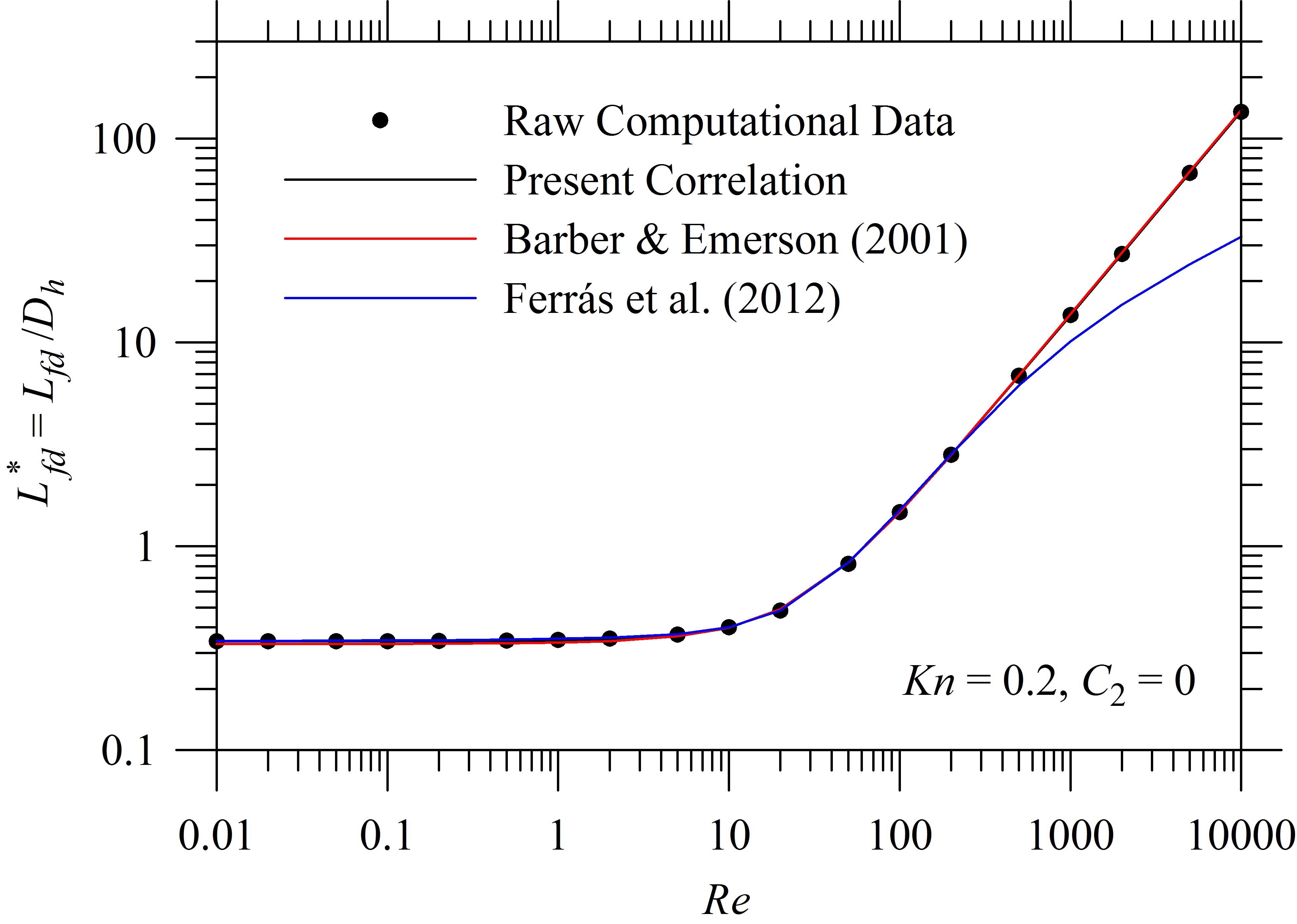
For pipe flows, however, no realistic comparison could be made since the only investigation from Barber and Emerson (4) recommended using the earlier correlations from Chen (17) and Dombrowski et al. (21) that were specifically developed for in the continuum regime, even for . Therefore, the present correlations in Eq. (19) are recommended for evaluating for both pipe and channel flows.
3.3 Incremental Pressure Drop Number
The investigation on pressure drop in the entrance region of micro-channels has been carried out by analysing the variations in as functions of for different operating conditions and their asymptotic behaviour in the fully-developed section has been analysed from the variations in as functions or , and . While for qualitatively remains similar to that for the no-slip case with and hence could still be functionally represented by the similar form in Eq. (19), substantial qualitative differences have been observed in the pressure drop data. In this section, the variations in and are critically examined and the correlations for the latter, that are extremely important for the evaluation of pressure drop for , are proposed.
For pipe flows with first order velocity slip condition at the wall, i.e., with , the variations in for different and are presented in Fig. 7, from which, it is evident that irrespective of and , always increases from at to its asymptotic value for the fully-developed flow as , or, to be precise, for . These variations are similar to that observed for with no-slip condition at the wall, although the magnitude of , as well as for a particular , reduces considerably with the increase in . The reduction in is due to the decrease in both , which, as shown in Eq. (15) and Fig. 2, is independent of and depends only on for a given , and the velocity gradient and hence the shear stress at the wall, which, other than and , also depends on , as demonstrated in Fig. 3. These effects are more prominent as increases beyond .


Similar variations in Fig. 8 for the second order velocity slip condition at the wall with , however, show some never reported interesting features. It is observed that as well as , particularly for higher , could even be negative, which, other than the already reported decrease in in Eq. (14), could be attributed to the reduction in wall shear stresses that occurs with the increase in both and (see Fig. 3). It may be recognised that a positive , which is most often the case in the continuum regime for and with the first order velocity slip condition (), implies that if one calculates the true pressure drop using rather than given in Eq. (16), one would underestimate , while a negative would lead to an overestimation of using the same method, which in certain cases, could be more acceptable than any underestimation.


Since negative values of are observed only for higher with the second order velocity slip condition at the wall, the variations in with for different and are presented in Fig. 9. The figure clearly shows that irrespective of , is always negative for , whereas for lower values of (specifically for and in Fig. 9), is always positive, although for always remains negative in the entrance region. Similar variations in and for , on the other hand, show that although is always negative at least in the developing region of the pipe, remains negative for lower (see cases with and in Fig. 9), while it increases with the increase in and eventually becomes positive for higher (see results for and in Fig. 9).


Similar variations in for , which lies in the border-line between the continuum and the slip flow regimes (55), with and are presented in Fig. 10 for different . For brevity, the intermediate results for and are not presented. The comparison of results in Figs. 7 – 10 clearly shows that although could be negative for higher , irrespective of and , it always remains positive as is reduced to . Most importantly, no negative , and hence , could be detected for the first order velocity slip condition at the wall, irrespective of and .


Another apparently inconsequential general observation from Figs. 7 – 10, which has not been mentioned so far, is that for a given combination of and , both for a particular and decrease substantially with the increase in . Such variations are, however, expected since according to Eq. (17), is defined as the difference between the true and the expected fully-developed pressure drops that is normalised with respect to , where by definition, for a given and the working fluid, is a linearly increasing function of . Therefore, any reduction in or does not necessarily imply a corresponding decrease in and as such, should always be calculated according to Eq. (18).
The aforementioned observations may be summarised as follows. The generalised slip boundary condition allows a positive tangential velocity component at the wall that, other than the operating conditions, depends on the axial location. As a consequence, with the increase in both and , the normal gradient of axial velocity at the wall decreases for a given combination of and . Therefore, the corresponding wall shear stress and hence as a consequence of Eq. (11), the local friction factor are reduced. Finally, certain operating conditions can produce sufficient velocity slip at the wall that, owing to the complex interaction of three terms in Eq. (17), may eventually lead to not only negative in the entrance region, but also a negative .


In order to demonstrate that the pressure drop characteristics for channel flows qualitatively remain nearly the same as that for pipe flows, the variations in as functions of are presented in Fig. 11 with for different and . Comparison of results in Figs. 9 and 11 adequately substantiates the claim and for brevity, no further variations in for channel flows is presented in this article. Nevertheless, it is also obvious from Figs. 7 – 11 that for both pipe and channel flows, the variations in are quite complex functions of and their nature strongly depends on the operating condition. Therefore, at this point, no general functional form could be proposed that would adequately describe the observed variations in and hence this issue has been left beyond the scope of the present investigation.


As mentioned earlier in section 2, for a duct length , the actual pressure drop may be evaluated according to Eq. (18) by substituting and . Therefore, similar to , is also considered as another important characteristic of the developing flow through ducts that takes into account the pressure drop in the entrance region. The variations in as functions of for different and are presented in Figs. 12 and 13 for pipe and channel flows, respectively. It is evident from the figures that the magnitude of decreases considerably with the increase in , and , although in the high regime, and appears to be a weak function of and . In addition, for lower , is less sensitive to the change in and the sensitivity increases with the increase in . Since these observations may be explained in view of the foregoing discussions, they are not repeated here for brevity.


Figures 12 and 13 also clearly show that for lower , irrespective of and , is always positive, whereas for , depending upon and , could assume either positive or negative values. However, as mentioned earlier, for the first order velocity slip condition at the wall (), or, even for lower , remains always positive for both pipe and channel flows, irrespective of and .
Nevertheless, irrespective of and , the variations in as functions of are still described by two asymptotes, where the low and the high asymptotes are given by and , respectively. Similar to and , and have been obtained directly from the simulated data for at and at , respectively. The obtained data for different and are presented in Table 2, from which it is evident that could assume either positive or negative values for both pipe and channel flows. On the other hand, for pipe flows is marginally negative only for higher and , while it remains always positive for channel flows for the investigated ranges of and . As a result, in Figs. 12 and 13 could not be consistently presented using the logarithmic scale and in order to highlight that assumes considerably smaller but non-zero values as on a linear scale, the variations of in these figures are presented only for the range .
Depending upon and , since and assume both positive and negative values, could not be represented by the form similar to that for in Eq. (19). Therefore, an alternative relation, that respects both low and high asymptotes, has been adopted in order to correlate :
| (24) |
where is a function of and . At this point, however, it is important to note that as , the wall shear stress and it has been found to be proportional to . Therefore, in this region is proportional to , according to the definitions of dimensionless variables. Similar consequence, although only in the convection dominated regime, could also be derived from the conventional boundary layer theory. Extensive numerical simulations show that for , varies from for , where the convective effects are insignificant, to as , where the axial diffusion is negligible. Therefore, for , the first term on the right hand side of Eq. (14) as and hence no grid-independent solution either for or could be obtained in this limit, although has been found to attain a grid-independent value (27). Further critical appreciation of this issue, arising out of the singularity in boundary conditions at the inlet, however, has been left beyond the scope of the present article.
Nevertheless, with the increase in , substantial velocity slip occurs at the wall for a given that not only reduces the wall shear stress and hence close to the inlet, but also it modifies the exponent to a great extent, from unity to reasonable fractional values, such that grid independent solutions for and hence could be obtained even in the limit as . Therefore, correlations for have been obtained only for , while accommodating the complete range of investigated .
In order to develop these correlations, however, and in Table 2 have been directly used, since owing to their large variations with and changing dependence on both and , no reliable correlation for them could be derived. Subsequently, has been determined for each combination of and , either by minimising the maximum absolute relative error in when for the entire range of , or using the least square method (i.e., by maximising the coefficient of determination ), when is expected for certain . The latter condition could be easily identified by checking i) if , where has been taken as , or ii) if the product of and is negative. Finally, for a given , as a function of has been expressed as:
| (25) |
where are functions of . For pipe flows, they have been correlated as:
| (26a) | |||||
| (26b) | |||||
| (26c) | |||||
Similarly for channel flows, could be expressed as:
| (27a) | |||||
| (27b) | |||||
| (27c) | |||||


Since the tabulated values of and have been used in order to evaluate , the correlations for in Eq. (24) are expected to perform extremely well for all simulated cases. Therefore, in order to demonstrate that these correlations are still accurate for the intermediate values of and , where and are required to be interpolated, four additional cases for both geometries have been carefully chosen between two tabulated results, where either or changes its sign. Comparison between the observed and the correlated values of for these additional cases are presented in Fig. 14. In addition, the results for two tabulated cases with and for are also shown in the same figure in order to demonstrate that the proposed correlations indeed perform extremely well for the already reported cases, where and could be directly obtained from Table 2 without any interpolation. While quantifying the performance of the correlations, however, it must be noted that since has been recorded for some of the cases, the maximum absolute relative error cannot be consistently considered an appropriate measure of deviation and hence the coefficient of determination has been reported in order to demonstrate the accuracy of the correlations.
At this point, a few comments regarding the interpolation of and for intermediate and are essential. It has been observed that the linearly interpolated and do not produce satisfactory agreement, owing to the non-linear nature of their variations as functions of both and . The minimum values of coefficient of determination have been obtained as for both pipe and channel flows,1111
11
Among four additional cases, has been observed for with and for pipe and channel flows, respectively. when linear interpolation is used while considering and as independent variables. In order to improve the prediction, and have been subsequently considered as independent variables for interpolation. Even then, the use of linear interpolation has resulted in for both geometries, although these data are not shown in Fig. 14 for brevity. Finally, cubic functions1212
12
In order to fit cubic functions, if possible, two points on either sides of the desired have been selected (e.g., for for pipe flow). Otherwise, depending upon the availability of data, three points on one side and one point on the other side of the desired have been chosen (e.g., for for both geometries). of and quadratic functions1313
13
Quadratic functions have been fitted preferably by selecting two points on the higher side and one point on the lower side of the desired (e.g., for ). In the absence of such data, one point on the higher side and two points on the lower side have been chosen (e.g., for ). of have been employed for interpolating and , that, rounded up to the fourth place of decimal, produce for all additional cases involving both geometries.
From the foregoing discussions, it is obvious that for a duct length , evaluation of the actual pressure drop from Eq. (18) requires accurate information about in the developing region. However, since no correlation for could be derived from the present investigation owing to its complex dependence on the operating conditions, few comments on the estimation of for would be useful. While selecting the pumping device and determining its power requirement for a particular micro-channel application, an overestimation is often considered more acceptable than any underestimation and hence in order to be on the safer side, could be estimated as:
| (28a) | |||||
| (28b) | |||||
It must be emphasised that , calculated from Eq. (28) for , should never be used for optimisation since the estimated value would always be greater than the true pressure drop and may be grossly erroneous. For , however, the correlation for in Eq. (24) may be used for accurately evaluating .
4 Summary, Conclusions and Final Remarks
In the present investigation, developing laminar flows through micro-capillaries and micro-channels have been numerically analysed by solving the conventional NS equations (5) – (7) along with the second-order velocity slip condition at the wall in Eq. (8). For both pipe and channel flows, thorough investigations have been conducted for and , while specifying and varying from to . The results for the first order velocity slip condition, similar to that presented by Barber and Emerson (4) and Ferrás et al. (28) for parallel plate channels, have been obtained by setting , whereas that of Durst et al. (27) in the continuum regime have been generated with .
Before carrying out the extensive parametric study, the maximum length of the computational domain has been first ascertained. The development of the axial velocity profile shows that analytical solutions for the fully-developed flow have always been obtained at the exit of the duct, irrespective of the operating condition. Since the obtained numerical solutions are also grid independent, this observation confirms the authenticity of the predicted results. The converged solutions for each combination of , and have been further post-processed in order to evaluate the local friction factor , the dimensionless development length , the local and the fully-developed incremental pressure drop number and , respectively. The obtained data have been carefully analysed and correlations for and have been proposed for both geometries. The major conclusions from the present investigation may be summarised as follows:
- 1.
The development of the axial velocity profile shows that although irrespective of , and , for any is always higher than , the velocity gradients at the wall and hence could be considerably less than that in the fully-developed section, particularly for higher and . These effects are more prominent for lower and significantly affect the variations in and hence . The velocity overshoots, on the other hand, are observed to be more pronounced for higher with lower velocity slip at the wall and are considerably reduced with the decrease in as well as the increase in both and .
- 2.
The development length increases with the increase in both and , except for pipe flows in the high regime and for both geometries in the low regime, but only with . For the first exception, initially decreases and subsequently increases with the increase in , except for , for which, although the variation is marginal, it decreases once again. For the second exception, on the other hand, decreases marginally for higher , which could be detected for for both geometries.
- 3.
Similar to the continuum regime, in the presence of ssecond order velocity slip at the wall is also characterised by the low and the high asymptotes and hence it has been correlated according to Eq. (19), where the expressions for , and are provided in Eqs. (20) – (23). The proposed correlations for produce % and % errors for pipe and channel flows, respectively. On the other hand, with a constant , as proposed by Durst et al. (27), these errors are obtained as % and %, respectively. Even for flows through parallel plate micro-channels with the first order velocity slip condition at the wall, the present correlation has been found to be more accurate than those proposed by Barber and Emerson (4) and Ferrás et al. (28) for the entire range of Reynolds number.
- 4.
Pressure drop characteristics in the entrance region as well as in the fully-developed section of micro-channels have been thoroughly analysed. It has been observed that depending upon the operating condition, particularly for higher and , both and could assume negative values. This important as well as interesting feature, which is more prominent in the low regime, has never been reported in the literature. These results imply that in the presence of substantial velocity slip at the wall, the pressure gradient in the developing section could be even less than that in the fully-developed region.
- 5.
No reliable correlation for could be proposed from the present investigation since for both geometries, is a quite complicated function of the axial location and the functional form depends strongly on the operating condition. Although the calculation of true pressure drop for a duct of length requires precise knowledge about , a method has been proposed in order to obtain an conservative estimate of the pressure drop that, other than the fully-developed friction factor , also depends on for .
- 6.
The magnitude of decreases consistently with the increase in , and , although it is a weak function of and in the high regime where . Irrespective of , it has been found to be a strong function of , whereas it appears to be weak function of for lower and its sensitivity to the change in increases with the increase in .
- 7.
Similar to , the variations in as functions of are also represented by the low and the high asymptotes, and , respectively for any combination of and . However, since these asymptotic values vary over a large range and their functional dependence on both and changes considerably over the investigated ranges, no reliable correlation for either or could be proposed. Moreover, since for both geometries and for pipe flows assume both positive and negative values, could not be expressed by the form similar to that for and hence an alternative expression in Eq. (24) has been adopted that satisfies both low and high limits. Using the tabulated values of and , has been determined for each , while allowing to vary from to , from which, correlations for has been proposed that are presented in Eqs. (25) – (27).
- 8.
Four additional cases for both geometries have been specifically simulated for intermediate values of and , where and are required to be carefully interpolated using cubic functions of and quadratic functions of . The performance of the proposed correlations show excellent agreement with the simulated data for all additional cases, with for both geometries.
As a final remark, it may be mentioned that in the present investigation, although , and have been varied over wide ranges, has been kept fixed to unity. Previous investigations and the present analysis based on the dimensionless parameters clearly show that the effects of and could not be separated if the first order velocity slip condition at the duct surface is applied. Therefore, in the future, in the second order velocity slip boundary condition at the wall should be varied over a realistic range in order to quantify its effects on both development length and pressure drop in the entrance region for pipe and channel flows.
References
- (1) C. K. Aidun and J. R. Clausen. Lattice-Boltzmann method for complex flows. Annual Review of Fluid Mechanics, 42:439–472, 2010.
- (2) S. Ansumali, I. V. Karlin, S. Arcidiacono, A. Abbas, and N. Prasianakis. Hydrodynamics beyond navierstokes: exact solution to the lattice Boltzmann hierarchy. Physical Review Letters, 98:124502, 2007.
- (3) E. B. Arkilic, M. A. Schmidt, and K. S. Breuer. Gaseous slip flow in microchannels. Journal of Microelectromechanical Systems, 6:167–174, 1997.
- (4) R. W. Barber and D. R. Emerson. A numerical investigation of low reynolds number gaseous slip flow at the entrance of circular and parallel plate micro-channels. In Proceedings of ECCOMAS Computational Fluid Dynamics Conference, 2001.
- (5) R. W. Barber and D. R. Emerson. Challenges in modeling gas-phase flow in microchannels: from slip to transition. Heat Transfer Engineering, 27:3–12, 2006.
- (6) A. Beskok and G. E. Karniadakis. Rarefaction and compressibility effects in gas microflows. ASME J. Fluids Eng., 118:448–456, 1996.
- (7) A. Beskok and G. E. Karniadakis. A model for flows in channels, pipes, and ducts at micro and nano scales. Microscale Thermophysical Engineering, 3:43–77, 1999.
- (8) G. A. Bird. Molecular gas dynamics and the direct simulation of gas flows. Clarendon Press, Oxford, 1994.
- (9) R. B. Bird, W. E. Stewart, and E. N. Lightfoot. Transport Phenomena. John Wiley & Sons, New York, 2002.
- (10) B. Y. Cao, J. Sun, M. Chen, and Z. Y. Guo. Molecular momentum transport at fluid-solid interfaces in mems/nems: a review. International Journal of Molecular Sciences, 10:4638–4706, 2009.
- (11) C. Cercignani. Theory and application of the Boltzmann equation. Scottish Academic Press, Edinburgh, 1975.
- (12) C. Cercignani. The Boltzmann equation and its applications. Springer-Verlag, New York, 1988.
- (13) C. Cercignani. Mathematical methods in kinetic theory. Plenum, New York, 1990.
- (14) C. Cercignani. Rarefied gas dynamics. Cambridge University Press, Cambridge, 2000.
- (15) S. Chakraborty and F. Durst. Derivations of extended navier-stokes equations from upscaled molecular transport considerations for compressible ideal gas flows: Towards extended constitutive forms. Phys. Fluids, 19:088104, 2007.
- (16) D. Chen and D. B. Bogy. Comparisons of slip-corrected reynolds lubrication equations for the air bearing film in the head-disk interface of hard disk drives. Tribology Letters, 37:191–201, 2010.
- (17) R. Y. Chen. Flow in the entrance region at low reynolds numbers. ASME J. Fluids Eng., 95:153–158, 1973.
- (18) S. Colin. Rarefaction and compressibility effects on steady and transient gas flows in microchannels. Microfluidics and Nanofluidics, 1:268–279, 2005.
- (19) S. Colin. Gas microflows in the slip flow regime: a critical review on convective heat transfer. ASME Journal of Heat Transfer, 134:020908, 2012.
- (20) R. Cornubert, D. d’Humieres, and D. Levermore. A knudsen layer theory for lattice gases. Physica D, 47:241–259, 1991.
- (21) N. Dombrowski, E. A. Foumeny, S. Ookawara, and A. Riza. The influence of reynolds number on the entry length and pressure drop for laminar pipe flow. The Canadian Journal of Chemical Engineering, 71:472–476, 1993.
- (22) N. Dongari, A. Agrawal, and A. Agrawal. Analytical solution of gaseous slip flow in long microchannels. Int. J. Heat Mass Transfer, 50:3411–3421, 2007.
- (23) N. Dongari, R. Sambasivam, and F. Durst. Extended navierstokes equations and treatments of micro-channel gas flows. Journal of Fluid Science and Technology, 4:454–467, 2009.
- (24) N. Dongari, F. Durst, and S. Chakraborty. Predicting microscale gas flows and rarefaction effects through extended navierstokesfourier equations from phoretic transport considerations. Microfluidics and Nanofluidics, 9:831–846, 2010.
- (25) N. Dongari, Y. H. Zhang, and J. M. Reese. Molecular free path distribution in rarefied gases. Journal of Physics D, Applied Physics, 44:125502, 2011a.
- (26) N. Dongari, Y. H. Zhang, and J. M. Reese. Modeling of knudsen layer effects in micro/nanoscale gas flows. ASME J. Fluids Eng., 133:071101, 2011b.
- (27) F. Durst, B. Ünsal, S. Ray, and O. Saleh. The development lengths of laminar pipe and channel flows. ASME J. Fluids Eng., 127:1154–1160, 2005.
- (28) L. Ferrás, A. Alfonso, M. Alves, J. Nóbrega, and F. Pinho. Development length in planar channel flows of newtonian fluids under the influence of wall slip. ASME J. Fluids Eng., 134:104503–1–104503–5, 2012.
- (29) J. H. Ferziger and M. Perić. Computational Methods for Fluid Dynamics. Springer, Berlin, 1999.
- (30) R. W. Fox, A. T. McDonald, and P. J. Pritchard. Introduction to Fluid Mechanics. John Wiley & Sons, New York, 2010.
- (31) M. Gad-el-Hak. The fluid mechanics of microdevices - the freeman scholar lecture. JFE, 121:5–33, 1999.
- (32) M. Gad-el-Hak. Flow physics in mems. Mécanique & Industries, 2:313–341, 2001.
- (33) M. Gad-el-Hak. Gas and liquid transport at the microscale. Heat Transfer Engineering, 27:13–29, 2006.
- (34) N. G. Hadjiconstantinou. Analysis of discretization in the direct simulation monte carlo. Phys. Fluids, 12:2634–2638, 2000.
- (35) N. G. Hadjiconstantinou. The limits of navierstokes theory and kinetic extensions for describing small-scale gaseous hydrodynamics. Phys. Fluids, 18:111301, 2006.
- (36) C. M. Ho and Y. C. Tai. Micro-electro-mechanical-systems (mems) and fluid flows. Annual Review of Fluid Mechanics, 30:579–612, 1998.
- (37) S. Jin and M. Slemrod. Regularization of the burnett equations via relaxation. Journal of Statistical Physics, 103:1009–1033, 2001.
- (38) S. G. Kandlikar, S. Colin, Y. P. S. Garimella, R. F. Pease, J. J. Brandner, and D. B. Tuckerman. Heat transfer in microchannels - 2012 status and research needs. ASME Journal of Heat Transfer, 135:091001, 2013.
- (39) G. E. Karniadakis and A. Beskok. Micro flows: fundamentals and simulation. Springer-Verlag, New York, 2002.
- (40) G. E. Karniadakis, A. Beskok, and N. Aluru. Microflows and Nanoflows: Fundamentals and Simulation. Springer-Verlag, New York, 2005.
- (41) P. K. Khosla and S. G. Rubin. A diagonally dominant second order accurate implicit scheme. Comput. Fluids, 2:207–209, 1974.
- (42) M. Knudsen. Die gesetze der molekularströmung und der inneren reibungsströmung der gase durch röhren. Annalen der Physik, 333(1):75–130, 1909.
- (43) B. Li and D. Y. Kwok. Discrete Boltzmann equation for microfluidics. Physical Review Letters, 90:124502, 2003.
- (44) C. R. Lilley and J. E. Sader. Velocity profile in the knudsen layer according to the Boltzmann equation. Proceedings of Royal Society A, 464:2015–2035, 2008.
- (45) D. A. . Lockerby and J. M. Reese. On the modelling of isothermal gas flows at the microscale. J. Fluid Mechanics, 604:235–261, 2008.
- (46) D. A. Lockerby, J. M. Reese, D. R. Emerson, and R. W. Barber. Velocity boundary condition at solid walls in rarefied gas calculations. Physical Review E, 70:017303, 2004.
- (47) S. K. Loyalka. Approximate method in kinetic theory. Phys. Fluids, 14:2291–2294, 1971.
- (48) L. S. Pan, G. R. Liu, and K. Y. Lam. Determination of slip coefficient for rarefied gas flows using direct simulation monte carlo. Journal of Micromechanics and Microengineering, 9:89–96, 1999.
- (49) S. V. Patankar. Numerical Heat Transfer and Fluid Flow. Hemisphere, Washington, DC, 1980.
- (50) S. V. Patankar and D. B. Spalding. A calculation procedure for heat, mass and momentum transfer in three-dimensional parabolic flows. Int. J. Heat Mass Transfer, 15(10):1787–1806, 1972.
- (51) C. Rhie and W. Chow. Numerical study of the turbulent flow past an airfoil with trailing edge separation. AIAA J., 21(11):1525–1532, 1983.
- (52) E. Roohi and M. Darbandi. Extending the navierstokes solutions to transition regime in two-dimensional micro- and nanochannel flows using information preservation scheme. Phys. Fluids, 21:082001, 2009.
- (53) R. Sambasivam. Extended Navier-Stokes Equations: Derivations and Applications to Fluid Flow Problems. PhD thesis, Friedrich Alexander Universität, Erlangen-Nürenberg, Germany, 2013.
- (54) M. Sbragaglia and Succi. Analytical calculation of slip flow in lattice Boltzmann models with kinetic boundary conditions. Phys. Fluids, 17:093602, 2005.
- (55) S. A. Schaaf and P. L. Chambre. Rarefied Gas Dynamics. Princeton University Press, Princeton, 1961.
- (56) R. K. Shah and A. L. London. Advances in Heat Transfer, Supplement I: Laminar Flow Forced Convection in Ducts. Academic Press, New York, San Francisco, London, 1978.
- (57) X. Shan, X. Yuan, and H. Chen. Kinetic theory representation of hydrodynamics: a way beyond the navierstokes equation. J. Fluid Mechanics, 550:413–441, 2006.
- (58) F. Sharipov. Application of the cercignani-lampis scattering kernel to calculations of rarefied gas flows. ii. slip and jump coefficients. European Journal of Mechanics B/Fluid, 22:133–143, 2003.
- (59) F. Sharipov and V. Seleznev. Data on internal rarefied gas flows. J Phys Chem Ref Data, 27:657–706, 1998.
- (60) C. E. Siewert and F. Sharipov. Model equations in rarefied gas dynamics: Viscous-slip and thermal-slip coefficients. Phys. Fluids, 14:4123–4129, 2002.
- (61) H. L. Stone. Iterative solution of implicit approximations of multidimensional partial differential equations. SIAM. J. Num. Anal., 5:530–541, 1968.
- (62) H. Struchtrup and M. Torrilhon. Regularization of grids 13 moment equations: derivation and linear analysis. Phys. Fluids, 15:2668–2680, 2003.
- (63) H. Struchtrup and M. Torrilhon. Higher-order effects in rarefied channel flows. Physical Review E, 78:046301, 2008.
- (64) G. H. Tang, Y. L. He, and W. Q. Tao. Comparison of gas slip models with solutions of linearized Boltzmann equation and direct simulation of monte carlo method. International Journal of Modern Physics C, 18:203–216, 2007a.
- (65) G. H. Tang, L. Zhuo, Y. L. He, and W. Q. Tao. Experimental study of compressibility, roughness and rarefaction influences on microchannel flow. Int. J. Heat Mass Transfer, 50:2282–2295, 2007b.
- (66) G. H. Tang, Y. H. Zhang, and D. R. Emerson. Lattice Boltzmann models for nonequilibrium gas flows. Physical Review E, 77:046701, 2008.
- (67) H. C. Weng and C. K. Chen. A challenge in navierstokes-based continuum modeling: Maxwell-burnett slip law. Phys. Fluids, 20:106101, 2008.
- (68) F. M. White. Fluid Mechanics. McGraw-Hill, New York, 2003.
- (69) L. Wu and D. B. Bogy. A generalized compressible reynolds lubrication equation with bounded contact pressure. Phys. Fluids, 13:2237–2244, 2001.
- (70) H. W. Zhang, Z. Q. Zhang, Y. G. Zheng, and H. F. Ye. Molecular dynamics-based prediction of boundary slip of fluids in nanochannels. Microfluidics and Nanofluidics, 12:107–115, 2012a.
- (71) J. Zhang. Lattice Boltzmann method for microfluidics: models and applications. Microfluidics and Nanofluidics, 10:1–28, 2011.
- (72) R. Zhang, X. Shan, and H. Chen. Efficient kinetic method for fluid simulation beyond the navierstokes equation. Physical Review E, 74:046703, 2006a.
- (73) W. Zhang, G. Meng, and X. Wei. A review on slip models for gas microflows. Microfluidics and Nanofluidics, 13:845–882, 2012b.
- (74) Y. H. Zhang, X. J. Gu, R. W. Barber, and D. R. Emerson. Capturing knudsen layer phenomena using a lattice Boltzmann model. Physical Review E, 74:046704, 2006b.
- (75) Y. Zheng, J. M. Reese, T. J. Scanlon, and D. A. Lockerby. Scaled navier-stokes-fourier equations for gas flow and heat transfer phenomena in micro- and nanosystems. In Proceedings of ASME ICNMM2006, Limerick, Ireland 96066, June 19–21 2006.
| Pipe | 0 | 0.6044 | 5.5935 | 0.6044 | 5.5935 | 0.6044 | 5.5935 | 0.6044 | 5.5935 | 0.6044 | 5.5935 | 0.6044 | 5.5935 |
|---|---|---|---|---|---|---|---|---|---|---|---|---|---|
| 0.0001 | 0.6045 | 5.5931 | 0.6045 | 5.5931 | 0.6045 | 5.5931 | 0.6045 | 5.5931 | 0.6045 | 5.5931 | 0.6045 | 5.5931 | |
| 0.001 | 0.6054 | 5.5882 | 0.6054 | 5.5884 | 0.6054 | 5.5884 | 0.6054 | 5.5882 | 0.6054 | 5.5882 | 0.6054 | 5.5882 | |
| 0.01 | 0.6136 | 5.5757 | 0.6138 | 5.5795 | 0.6141 | 5.5840 | 0.6144 | 5.5888 | 0.6146 | 5.5934 | 0.6149 | 5.5981 | |
| 0.02 | 0.6220 | 5.5795 | 0.6232 | 5.5975 | 0.6244 | 5.6159 | 0.6256 | 5.6344 | 0.6268 | 5.6543 | 0.6281 | 5.6743 | |
| 0.05 | 0.6399 | 5.5918 | 0.6471 | 5.6894 | 0.6544 | 5.7903 | 0.6623 | 5.8943 | 0.6703 | 6.0014 | 0.6786 | 6.1116 | |
| 0.1 | 0.6531 | 5.5768 | 0.6756 | 5.8708 | 0.6999 | 6.1890 | 0.7263 | 6.5322 | 0.7550 | 6.9053 | 0.7866 | 7.3167 | |
| 0.15 | 0.6554 | 5.5253 | 0.6951 | 6.0496 | 0.7398 | 6.6360 | 0.7907 | 7.3044 | 0.8501 | 8.0913 | 0.9240 | 9.0654 | |
| 0.2 | 0.6524 | 5.4554 | 0.7092 | 6.2142 | 0.7751 | 7.0958 | 0.8538 | 8.1542 | 0.9555 | 9.5227 | 1.1160 | 11.6313 | |
| Channel | 0 | 0.3152 | 1.0984 | 0.3152 | 1.0984 | 0.3152 | 1.0984 | 0.3152 | 1.0984 | 0.3152 | 1.0984 | 0.3152 | 1.0984 |
| 0.0001 | 0.3152 | 1.0985 | 0.3152 | 1.0985 | 0.3152 | 1.0985 | 0.3152 | 1.0985 | 0.3152 | 1.0985 | 0.3152 | 1.0985 | |
| 0.001 | 0.3156 | 1.0992 | 0.3156 | 1.0992 | 0.3156 | 1.0992 | 0.3156 | 1.0992 | 0.3156 | 1.0992 | 0.3156 | 1.0992 | |
| 0.01 | 0.3198 | 1.1130 | 0.3199 | 1.1133 | 0.3200 | 1.1136 | 0.3200 | 1.1140 | 0.3201 | 1.1144 | 0.3202 | 1.1148 | |
| 0.02 | 0.3241 | 1.1337 | 0.3245 | 1.1359 | 0.3249 | 1.1383 | 0.3254 | 1.1409 | 0.3258 | 1.1434 | 0.3262 | 1.1461 | |
| 0.05 | 0.3338 | 1.1950 | 0.3364 | 1.2105 | 0.3391 | 1.2265 | 0.3419 | 1.2429 | 0.3447 | 1.2597 | 0.3476 | 1.2766 | |
| 0.1 | 0.3417 | 1.2740 | 0.3502 | 1.3277 | 0.3591 | 1.3839 | 0.3683 | 1.4422 | 0.3780 | 1.5027 | 0.3879 | 1.5655 | |
| 0.15 | 0.3436 | 1.3248 | 0.3590 | 1.4279 | 0.3751 | 1.5378 | 0.3920 | 1.6537 | 0.4096 | 1.7763 | 0.4280 | 1.9059 | |
| 0.2 | 0.3425 | 1.3549 | 0.3647 | 1.5129 | 0.3880 | 1.6821 | 0.4123 | 1.8636 | 0.4377 | 2.0565 | 0.4647 | 2.2658 | |
| Pipe | 0.0001 | 76.3599 | 1.2655 | 76.3526 | 1.2655 | 76.3453 | 1.2655 | 76.3380 | 1.2655 | 76.3307 | 1.2655 | 76.3234 | 1.2655 |
| 0.001 | 63.2900 | 1.2454 | 62.9725 | 1.2453 | 62.6644 | 1.2453 | 62.3652 | 1.2452 | 62.0746 | 1.2451 | 61.7920 | 1.2450 | |
| 0.01 | 31.4299 | 1.0866 | 29.5644 | 1.0850 | 28.2273 | 1.0835 | 27.1745 | 1.0822 | 26.3005 | 1.0810 | 25.5503 | 1.0798 | |
| 0.02 | 21.6288 | 0.9478 | 19.4039 | 0.9439 | 18.0081 | 0.9403 | 16.9569 | 0.9369 | 16.1016 | 0.9335 | 15.3752 | 0.9302 | |
| 0.05 | 10.9205 | 0.6591 | 8.5012 | 0.6449 | 7.1769 | 0.6312 | 6.2058 | 0.6176 | 5.4263 | 0.6043 | 4.7707 | 0.5911 | |
| 0.1 | 5.3864 | 0.4029 | 3.0287 | 0.3709 | 1.8488 | 0.3403 | 1.0098 | 0.3109 | 0.3544 | 0.2826 | 0.2554 | ||
| 0.15 | 3.2671 | 0.2712 | 1.0311 | 0.2254 | 0.1831 | 0.1439 | 0.1075 | 0.0737 | |||||
| 0.2 | 2.2047 | 0.1948 | 0.0940 | 0.1391 | 0.0896 | 0.0456 | 0.0062 | ||||||
| Channel | 0.0001 | 80.3390 | 0.6802 | 80.3745 | 0.6912 | 80.3672 | 0.6912 | 80.3599 | 0.6912 | 80.3526 | 0.6912 | 80.3453 | 0.6912 |
| 0.001 | 67.2768 | 0.6726 | 66.9628 | 0.6814 | 66.6541 | 0.6813 | 66.3544 | 0.6813 | 66.0632 | 0.6812 | 65.7801 | 0.6812 | |
| 0.01 | 35.1348 | 0.6086 | 33.2312 | 0.6110 | 31.8826 | 0.6101 | 30.8196 | 0.6093 | 29.9364 | 0.6086 | 29.1775 | 0.6079 | |
| 0.02 | 25.0101 | 0.5505 | 22.7359 | 0.5513 | 21.3181 | 0.5496 | 20.2478 | 0.5480 | 19.3757 | 0.5466 | 18.6339 | 0.5452 | |
| 0.05 | 13.5077 | 0.4184 | 11.0197 | 0.4147 | 9.6489 | 0.4088 | 8.6385 | 0.4030 | 7.8251 | 0.3974 | 7.1392 | 0.3918 | |
| 0.1 | 7.1224 | 0.2825 | 4.6717 | 0.2700 | 3.4163 | 0.2555 | 2.5153 | 0.2415 | 1.8063 | 0.2279 | 1.2214 | 0.2147 | |
| 0.15 | 4.5213 | 0.2055 | 2.1511 | 0.1823 | 1.0139 | 0.1606 | 0.2249 | 0.1401 | 0.1209 | 0.1028 | |||
| 0.2 | 3.1242 | 0.1522 | 0.8822 | 0.1252 | 0.0984 | 0.0740 | 0.0519 | 0.0317 | |||||