Effective dielectric response of dispersions of graded particles

The effective properties of dispersions of graded particles have been studied intensively. Besides being important due to their abundance in nature [1], such systems attract particular interest because of their potential technical applications. For instance, the effective dielectric response of graded composites can be tuned finely by designing the dielectric profiles of the constituent. Numerous applications of such systems are discussed in [2, 3, 4, 5, 6, 7, 8, 9].

Despite serious efforts made so far, the determination of the effective dielectric properties of dispersions of graded particles, which is the objective of the present report, remains a challenging theoretical problem, even in the quasistatic limit. The reason is strong variations of the electric field in such systems due to electromagnetic interactions and spatial correlations of their constituents. As a result, reliable analytical results, such as [10, 11, 12, 13] for graded spherical inclusions or [14, 15, 16] for two-dimensional composites of graded cylindrical inclusions, are rare and have been obtained within the Maxwell-Garnett approach [17, 18, 19] for diluted low-contrast dispersions, where the interparticle influences are negligibly weak: the problem is actually reduced to solving the governing equation for the electric potential of a single particle in a uniform external field [10, 11, 12, 13, 14, 15, 16]. Similarly, computer simulations [20] deal with the response of a single graded particle in the computational domain. This situation tacitly implies the use of the Maxwell-Garnett type of homogenization.

The results [11, 12, 13, 14] validated approximate schemes known as the differential effective dipole approximation (DEDA) [21, 22], anisotropic differential effective dipole approximation (ADEDA) [23], and differential effective multipole moment approximation (DEMMA) [21, 24]. Based on the application of differential analysis to available rigorous solutions for a single graded particle, these schemes allowed one to evaluate the induced dipole moments of single graded particles with more complex shapes and, in general, anisotropic permittivity profiles. The differential analysis also became an integral part of other approaches, such as the differential replacement procedure (DPR) [25], which combines it with an energy equivalency condition; the multiscale homogenization scheme [26], proceeding from a generic theorem on the equivalence between a graded dielectric ellipsoid and an anisotropic homogeneous ellipsoid, etc.

It is significant to emphasize that after the individual polarizability of a graded particle is found with the just-listed or similar methods, the effective permittivity of a dispersion of such particles is calculated using again the Maxwell-Garnett approach. As the filler particle concentration or the particle-matrix contrast or both are increased, the electric field distribution in the dispersion becomes extremely complicated and difficult to visualize. The pertinent microscopic calculations, which now require the knowledge of an infinite set of the correlation functions of the system, become virtually impossible.

By this report, we would like to attract the Reader’s attention to new developments of our earlier results [27, 28, 29] and their applications to dispersions of graded hard dielectric spheres with piecewise-continuous permittivity profiles. They are obtained using our original method of compact groups of inhomogeneities [27, 28, 29]. It is designed to effectively take into account many-particle polarization and correlation effects in a system with complex microstructure without uncontrolled assumptions about them. The essential details of the method are presented in section II. The equation for the effective dielectric constant of the dispersions is derived in section III. This equation still contains an unknown parameter, the permittivity of the host in the auxiliary system; combining our approach with the Hashin–Shtrikman variational theorem [30], this parameter is determined in section IV. The results of contrasting our theory with other authors’ analytical and numerical results are given in section V. The application of the theory to nonconducting dispersions of core-shell particles are discussed in section VI. The main results obtained and further suggestions are summarized in section VII.

The main points of this approach are as follows.

(1) The effective quasistatic permittivity $\varepsilon_{\rm{eff}}$ of a system is defined by the relation [19]

where ${\bf{D}}({\bf{r}})$, ${\bf{E}}({\bf{r}})$, and $\varepsilon({\bf{r}})$ are the local values of, respectively, the electric induction, electric field, and permittivity in the system. The angle brackets in (1) mean either statistical averaging or averaging by volume integration; for an infinite system, both ways are expected to give, according to the ergodic hypothesis [19, 8], the same result.

(2) A dispersion $\cal{D}$ to be homogenized is equivalent, in its long-wave dielectric response, to an auxiliary system $\cal{S}$ prepared by embedding the constituents (particles and matrix) of $\cal{D}$ into a host (perhaps, imagined), $\cal{M}$, of some permittivity $\varepsilon_{\rm f}$. The system $\cal{S}$ can be viewed as a set of compact groups of particles and regions occupied by the real matrix. The compact groups are defined as macroscopic regions whose typical sizes are much smaller than the wavelength $\lambda$ of probing radiation in $\cal{M}$, but which yet include sufficiently large numbers $N$ of particles to remain macroscopic and retain the properties of the entire $\cal{S}$. The permittivity distribution in $\cal{S}$ is

where $\delta\varepsilon(\bf{r})$ is the contribution from a compact group located at point $\bf{r}$. The explicit form of $\delta\varepsilon({\bf{r}})$ is modeled in accord with the geometrical parameters and dielectric properties of $\cal{D}$’s constituents.

(3) The analysis of the electric field distribution in a system with permittivity distribution (2) is based on the equation describing the propagation of an electromagnetic wave in inhomogeneous media. After this equation is replaced by an equivalent integral equation, the formal solutions for the electric field and induction are represented in the form of infinite iterative series. In the limit $\lambda\to\infty$, fluctuations of particle numbers in compact groups and correlations between the particles in different groups are negligibly small, whereas the groups themselves are actually, with respect to the probing radiation, one-point inhomogeneities. Their contributions are formed by those ranges of coordinate values where the electromagnetic field propagators reveal a singular behavior. Decomposing each propagator into a Dirac delta function part and a principal value part (see the end of section IV), and using symmetry reasoning, the averaged contributions from compact groups to $\langle{\bf{E}}\rangle$ and $\langle{\bf{D}}\rangle$ can be singled out from all terms in the iterative series for ${\bf{E}}({\bf{r}})$ and ${\bf{D}}({\bf{r}})$. These contributions are shown to dominate in the formation of the long-wavelength dielectric characteristics of the system. As a result, for macroscopically homogeneous and isotropic systems we have

where $\textbf{E}_{0}$ is the amplitude of the incident wave field in ${\cal M}$. For models with bounded and piecewise-continuous $\delta\varepsilon({\rm{\bf r}})$, Eqs. (3) and (4) are rigorous in the quasistatic limit. In particular, together with Eq. (1) they reproduce the classical result [19]

which is valid, to $O\left(\left(\varepsilon-\overline{\varepsilon}\right)^{2}/\overline{\varepsilon}^{2}\right)$, for any mixture in which the local deviations of permittivity $\varepsilon$ from the average value $\overline{\varepsilon}$ [$=\varepsilon_{\rm f}+\langle\delta\varepsilon({\rm\bf r})\rangle$] are weak.

Thus, the analysis of $\varepsilon_{\rm eff}$ reduces to modeling $\delta\varepsilon({\rm{\bf r}})$, calculating its moments $\langle\left({\delta\varepsilon({\rm{\bf r}})}\right)^{s}\rangle$, finding the sums in Eqs. (3) and (4), and deciding on the value of $\varepsilon_{\rm f}$.

For a dispersion of inhomogeneous hard dielectric spheres, with radius $R$ and piecewise-continuous permittivity profile $\varepsilon_{1}=\varepsilon_{1}({\bf r})$, embedded in a uniform matrix, with constant permittivity $\varepsilon_{0}$,

where $\Delta\varepsilon_{0}=\varepsilon_{0}-\varepsilon_{\rm f}$, $\Delta\varepsilon_{1}({\bf{r}})=\varepsilon_{1}({\bf{r}})-\varepsilon_{{\rm f}}$, $\theta(x)$ is the Heaviside step function, and the summation is carried out over the position vectors ${\bf{r}}_{a}$ of $N$ spheres belonging to the compact group at ${\bf{r}}$.

For this $\delta\varepsilon({\rm{\bf r}})$, both direct volume integration [28, 29] and statistical averaging [31] give

where $n=N/V$ and $c=4\pi R^{3}n/3$ are the number density and volume concentration of spheres, respectively, and the integral is taken over the sphere volume $\Omega$. Then the sums in Eqs. (3) and (4) are found readily and together with Eq. (1) give [29]

In the case of isotropic spheres with radially-symmetric permittivity profile $\varepsilon_{1}=\varepsilon_{1}(r)$, Eq. (7) can be represented as

where $u=r/R$ is the dimensionless variable and $\varepsilon_{1}(u)$ is the sphere’s permittivity profile as a function of $u$.

For uniform spheres with $\varepsilon_{1}={\rm const}$, Eqs. (7) and (8) reduce to the classical Maxwell-Garnett mixing rule [17, 18] if $\varepsilon_{\rm f}=\varepsilon_{0}$, and the Bruggeman mixing rule [32, 33, 34] if $\varepsilon_{\rm f}=\varepsilon_{\rm eff}.$ These choices of $\varepsilon_{\rm f}$ are known as the Maxwell-Garnett and the Bruggeman types of homogenization, respectively. Which one must be used in a particular case has been a matter of long-lasting discussions (see, for instance, [2, 3, 4, 6, 7, 8]). To determine $\varepsilon_{\rm f}$ self-consistently, we use the idea [35] to combine the compact group approach with the Hashin-Shtrikman variational theorem [30] and require that two different ways of homogenization – through the linear relation (1) and through the equality of the electrostatic energies stored in $\cal{D}$ and $\cal{S}$ – give equal results.

Typically, theorem [30] is used to determine the most restrictive bounds for $\varepsilon_{\rm eff}$ of macroscopically homogeneous and isotropic two-constituent materials which can be derived in terms of the (definite) constituent permittivities and volume concentrations. Attempts to make use of it to evaluate these bounds for heterogeneous media with graded constituents were made, for example, in [36, 25] by introducing comparison materials with microstructures different from those of the considered heterogeneous media.

Let ${\bf E}_{0}$ and

be the electric field and induction in ${\cal M}$ filling a large region of volume $V$, provided the region’s boundary ${\cal B}$ is maintained at a prescribed time-independent potential $\psi({\cal B})=\psi_{0}({\cal B})$ and there are no free charges inside. Next, suppose that the whole of the region is changed to a material with permittivity (2), but without changing $\psi({\cal B})$ and adding free charges. Then, according to the Hashin-Shtrikman variational theorem [30], the functional (of ${\bf{T}}\equiv{\bf{D}}-\varepsilon_{\rm f}{\bf{E}}$)

subject to the subsidiary condition

is stationary for

and its stationary value $U_{\textbf{T}}^{\rm s}$ is the electrostatic energy stored in $V$.

Note that Eq. (12) is equivalent to

where $\varepsilon({\bf{r})}=\varepsilon_{\rm f}+\delta\varepsilon({\bf{r}})$, and Eq. (11) is fulfilled.

In view of Eq. (12), the integrand in Eq. (10) reduces to $\varepsilon_{\rm f}\textbf{E}^{2}_{0}+\left(\varepsilon-\varepsilon_{\rm f}\right)\textbf{E}\textbf{E}_{0}$. Hence, using Eqs. (1) and (3) and denoting

we find

It is natural to require that this value be equal to the electrostatic energy stored in the homogenized system. Then, in view of Eqs. (1) and (3), we also have

Finally, Eqs. (1), (3), and (4) yield

Eqs. (14), (15), and (16) give a system of homogeneous linear equations in $\varepsilon_{\rm f}$ and $\varepsilon_{\rm eff}$:

The nontrivial solutions exist provided

In the case

$\varepsilon_{\rm f}=\varepsilon_{\rm eff}$. If $\langle Q\rangle=1$, then $\varepsilon_{\rm f}=-2\varepsilon_{\rm eff}$. The latter situation may occur for metamaterials [37, 38], but is beyond the scope of the present work.

It follows that within the compact group approach supplemented by the Hashin-Shtrikman theorem [30], both ways of homogenization (through the linear relation between the average induction and average field, and through the equality of the electrostatic energies of the heterogeneous and homogenized systems) are consistent provided the Bruggeman-type homogenization $\varepsilon_{\rm f}=\varepsilon_{\rm eff}$ is used. The looked-for $\varepsilon_{\rm eff}$ is the solution to Eq. (20). No special assumptions about the composition of the system, the geometry and concentration of the constituents, and the permittivity distribution (except for its piecewise continuity) in the system were used in the above discussion.

It should be emphasized that our approach is not equivalent to the classical Bruggeman mean-field approximation [32] (and for this reason, the term ”Bruggeman-type homogenization” is used for the result $\varepsilon_{\rm f}=\varepsilon_{\rm eff}$). The latter approximation is traditionally understood as a one-particle approach where a single particle is placed in the effective medium of permittivity $\varepsilon_{\rm eff}$ (see [3]). In contrast, our theory effectively incorporates many-particle effects, and the result $\varepsilon_{\rm f}=\varepsilon_{\rm eff}$ is derived for the situation where a macroscopically-large (compact) group of particles is placed in the effective medium of permittivity $\varepsilon_{\rm eff}$. It is the effects of interparticle polarizations and correlations in such groups that determine the behavior of $\varepsilon_{\rm eff}$ in the limit $\lambda\to\infty$.

Note that Eq. (20) can be represented as

This is exactly the condition $\langle\xi({\bf r})\rangle=0$ imposed on the stochastic field $\xi({\bf r})=(\varepsilon({\bf r})-\varepsilon_{\rm f})/(2\varepsilon_{\rm f}+\varepsilon({\bf r}))$ in the strong-property-fluctuation theory (SPFT) [7, 39, 40, 41, 42, 43, 44, 45, 46] in order to improve the convergence of the iteration procedure applied to an integral equation for $\bf E({\bf r})$. The resulting Dyson-type equation for $\langle{\bf E}({\bf r})\rangle$ is usually analyzed using the second-order truncation of the mass operator series (bilocal approximation [7, 40, 43, 44, 45]; on the significance of the third-order approximation, see [46]), the Gaussian statistics for $\xi({\bf r})$, and model expressions for the two-point correlation function $G({\bf r},{\bf r^{\prime}})=\langle\xi({\bf r})\xi({\bf r^{\prime}})\rangle$. The symmetry of $G({\bf r},{\bf r^{\prime}})$ dictates the shape of the exclusion volume required for the decomposition of the propagator into a principal value part and a Dirac delta function part.

Contrastingly, in the compact group approach we use, for the propagators in the iterative series for $\textbf{E}(\textbf{r})$ and $\textbf{D}(\textbf{r})$, the decomposition with a spherical exclusion volume, in conformity with the requirement that both the entire system and compact groups be macroscopically homogeneous and isotropic. The statistical microstructure of the system comes into play only at the final stage, as the moments $\langle\left(\delta\varepsilon(\textbf{r})\right)^{s}\rangle$ are calculated.

For dispersions of spheres with permittivity profiles $\varepsilon_{1}=\varepsilon_{1}({\bf r})$ and $\varepsilon_{1}=\varepsilon_{1}({r})$, Eq. (20) reduces to, respectively, Eqs. (7) and (8) at $\varepsilon_{\rm f}=\varepsilon_{\rm eff}$ (then their right sides vanish).

For low values of volume concentration $c$ and dielectric contrast $\varepsilon_{1}/\varepsilon_{0}$, when both electromagnetic interactions and spatial correlations are small, the Maxwell-Garnett- and Bruggeman-type approaches are expected to give close results. This gives a good reason to contrast our theory with that [10] for mixtures of hard spheres with continuous radial permittivity profiles. Two ways were used there to calculate the polarizability of small inhomogeneous spheres in a quasistatic field and then $\varepsilon_{\rm eff}$: the internal field method to find the dipole moment by integrating the product of the field and the permittivity over the sphere’s volume, and the external field method to determine the field perturbation due to the sphere and then the amplitude of the equivalent dipole. Both ways lead to the same results, found by solving differential equations analytically; therefore, results [10] are free of ambiguities typical of computer simulations using the finite-difference method (see, for instance, [47]).

Figure 1 represents our results obtained with Eq. (8) for $\varepsilon_{\rm eff}$ of dispersions of hard dielectric spheres embedded in a medium of permittivity $\varepsilon_{0}=1$. The spheres have the following permittivity profiles ($0\leq u\leq 1$): homogeneous $\varepsilon_{1}(u){=2\,\varepsilon_{0}}$ (denoted as H); linear $\varepsilon_{1}(u)=\varepsilon_{0}(2-u)$ (L); parabolic $\varepsilon_{1}(u)=\varepsilon_{0}\left(2-u^{2}\right)$ (P). The agreement of our results with analytical results [10] turns out to be surprisingly good in the entire interval $c\in[0,0.4]$, investigated in [10]. It follows that our theory works well even in the situation where the concept of compact groups may seem questionable.

This fact is further confirmed by the comparison of our theory with analytical [12, 13] and simulation [20] results for hard dielectric spheres with the power-law permittivity profiles $\varepsilon_{1}(u)=c(b+u)^{k}$; those results are shown in Fig. 2 for $c=1$, $b=2$, and $k=0.25,\,0.5,\,1,\,2$. In [12, 13], the local electrical potentials for isolated spheres were derived rigorously in terms of the hyper-geometric function; then they were used to predict, based on the Maxwell-Garnett approach, the effective dielectric response of the graded composites in the dilute limit. The authors of [20] reported their effective permittivity calculations with the finite-element method for two-phase graded composite materials. The agreement between predictions [13] and simulation data [20] is sufficiently good only for low-contrast dispersions ($c=1$, $b=2$, and $k=0.25,\,0.5$), or in the dilute limit. As Fig. 2 reveals, our theory reproduces these results as well. For higher contrasts $\varepsilon_{1}/\varepsilon_{0}$ ($k=1$ and 2), the discrepancies between the theories become considerable. Our predictions for $\varepsilon_{\rm eff}$, given by Eq. (8) with $\varepsilon_{\rm f}=\varepsilon_{\rm eff}$, are always greater than those reported in [12, 13, 20]. This can be explained by the fact that our theory effectively takes into account multiparticle effects, whereas the studies [12, 13, 20] are actually one-particles approaches. It is interesting to note that for all above $k$’s, the formal use of the Maxwel-Garnett type of homogenization within our formalism [Eq. (8) with $\varepsilon_{\rm f}=\varepsilon_{0}$] gives results that are close to simulation data [20].

One of the practical applications of our theory is the prediction of the dielectric properties of microelectronic and optoelectronic devices requiring, for their superior performance, the use of packing materials with low dielectric constants, low dielectric losses, and high volume resistivities [5]. Since packaging materials are often polymer-ceramic composites, numerous core-shell theories have been developed (see, for instance, [48, 49, 50, 51, 52, 53] and literature therein) in which $\varepsilon_{\rm eff}$ of a composite is characterized by the geometric and permittivity parameters of the polymer phase, the filler phase, and an interphase region within the composite system. The equation for $\varepsilon_{\rm eff}$ is usually derived in these theories in several steps: (1) combining the particle and the adjacent interphase layer into a “complex particle”; (2) finding the effective polarizability of the isolated complex particle in a uniform field; (3) calculating the effective dielectric constat of the system within the standard one-particle approaches [17, 18, 32, 33, 19] or their modifications. In contrast, we use only step (1) and then calculate $\varepsilon_{\rm eff}$ treating the system in terms of compact groups of such complex particles.

Suppose that each filler particle, of radius $R$ and permittivity $\varepsilon_{1}$, is surrounded by a concentric particle-matrix interphase shell, of inner radius $R$, outer radius $R+t$, and permittivity $\varepsilon_{2}$. Considering the particle and the adjacent interphase shell to be a single hard particle, we readily find from Eq. (8) the equation for $\varepsilon_{\rm eff}$ of dispersions obtained by embedding such particles into a matrix of permittivity $\varepsilon_{0}$:

Here, $\delta=t/R$ is the relative thickness of the shell, and $\phi(c,\delta)$ is the effective volume concentration of complex particles (that is, the sum of the volume concentration $c$ of the filler and that of the interphase region). For hard filler particles,

Note that Eq. (22), but with different $\phi(c,\delta)$, also holds in the case where the interphase shells can be treated as fully penetrable (freely-overlapping) [54] (see also [55]). For such systems, the scaled-particle estimate [56] gives

As $\delta\to 0$, $\phi(c,\delta)=(1+3\delta+3\delta^{2})c+O(c\delta^{3})$ and tends to the value (23).

Figure 3 represents the results obtained with Eq. (22) for $\varepsilon_{\rm eff}$ of model epoxy-based polymer-ceramic composites [50], considered as dispersions of dielectric core-shell spheres. When processing the data, we took into account that: (1) the dielectric properties of constituents can change in the composite preparation process; (2) homogenization theories are intended to provide justified functional relationships between $\varepsilon_{\rm eff}$ and the parameters of the actual microstructure units in a real composite. For equal-sized spheres with $R=4.5\,{\rm\mu m}$ and $t=270\,{\rm nm}$ [50], the relative thickness $\delta=0.06$. As is seen from Fig. 3, our theory exactly recovers this value of $\delta$. It also predicts a drop, to $\varepsilon_{2}=2.5$, in the interphase permittivity, as compared to the matrix permittivity. This estimate differs from that given by theory [49], $\varepsilon_{2}=2.88$, by about 15%. Physically, the drop in $\varepsilon_{2}$ can be attributed [50] to the chemical bonding of the polymer to the filler particle surface.

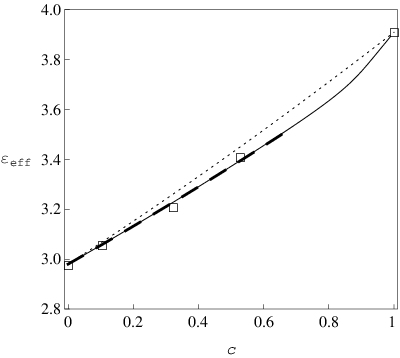
It should be remarked that the relation of the parameter $\delta$, calculated with the model of equal-sized spheres, to the actual thickness $d$ of the interphase in a real dispersion can be rather complicated due to the distribution of particle diameters and shapes. In particular, applying our general results [29] to mixtures of hard core-shell particles (not necessarily spherical) with different core sizes $R_{a}$ and fixed interphase thickness $d\ll R_{a}$, it is readily to show that $\varepsilon_{\rm eff}$ of such mixtures is given by Eq. (22), but with $\phi=c(1+S_{\rm p}d/V_{\rm p})$ instead of (23). Here $V_{\rm p}$ and $S_{\rm p}$ are the total volume and the total surface area of the particles, respectively. Correspondingly,

A convincing example in favor of this relation was given in [50]: after the actual particle size distribution of ${\rm SiO_{2}}$ particles was taken into account, the estimate $d\approx 5\,{\rm nm}$ was obtained. The latter is consistent with available literature data (see [50] for references).

To finish, we also test the applicability of our theory to high-contrast systems, such as polystyrene-barium titanate composites [57] (see also [48]). Experimental data [57] are widely-cited, but the parameters used to process them with existing theories and the results obtained differ considerably. For example, for $\varepsilon_{0}=2.55$, some reported values of $\varepsilon_{1}$ are 250 [58, 53] and 800 [48, 52], those of $\varepsilon_{2}$ are 3 [48], 7.24 [53], and 25 [52], and those of $\delta$ are 0.005 [48], 0.025 [recovered from Eq. (6) in [53] at $k=0.161$], and 0.26 [52]. Our estimates (see Fig. 4) fall in these ranges. This means that the functional structure of Eq. (22) is capable of reproducing available experimental data. However, an in-depth analysis of possible factors (size and shape distributions, dielectric losses, inhomogeneities of the interphase, etc.) behind the above discrepancies is beyond the scope of the present report.

The main results of this report can be summarized as follows.

(1) Combining the compact group approach [27, 28, 29] with the Hashin-Shtrikman variational theorem [30] and requiring that the two common ways for homogenization (through the linear material equation between the induction and the field, and through the equality of the electric energies of the heterogeneous and homogenized systems) give equal results, we proposed a new solution, which effectively incorporates many-particle effects in concentrated systems, to the problem of the effective quasistatic permittivity $\varepsilon_{\rm eff}$ of dispersions of graded dielectric particles. According to it: a dispersion to be homogenized is dielectrically equivalent to a macroscopically homogeneous and isotropic system prepared by embedding the constituents of the real dispersion into an imagined medium having the looked-for permittivity (Bruggeman-type homogenization); the equation for $\varepsilon_{\rm eff}$ is an integral relation obtained from Eq. (20) by summing up the statistical moments for the local deviations of the permittivity distribution in the model system from $\varepsilon_{\rm eff}$; this equation validates the condition postulated for the relevant stochastic field in the SPFT. The latter fact is a strong argument for our theory because the SPFT has proved to be very efficient for homogenization of composites of non-graded constituents.

(2) The efficiency of our theory was demonstrated by contrasting its results with analytical results [10, 12, 13] and simulation data [20] for dispersions of hard dielectric spheres with power-law permittivity profiles. The theory was also applied to nonconducting polymer-ceramic composites considered as dispersions of dielectric core-shell spheres. The comparison of its results with experimental data [48, 50, 57] showed that the theory can be used to predict the effective dielectric response of such systems in terms of the geometric and dielectric parameters of their constituents, including the interphase regions.

The generalizations of these results are possible in two directions, at least. First, the compact group approach is expected to be applicable to multiconstituent dispersions of anisotropic inhomogeneous dielectric particles, as long as these dispersions remain macroscopically homogeneous and isotropic. Some relevant general results for $\varepsilon_{\rm eff}$ of such systems are presented in [29]. Second, this approach can be extended to dispersions of particles with complex permittivities. In particular, it has already been shown to be efficient for the description of electric percolation phenomena in composites of core-shell particles [54], two-step electrical percolation in nematic liquid crystals filled with multiwalled carbon nanotubes [55], and the effective structure parameters of suspensions of nanosized insulating particles [59].