Our modeling of the OH^- near-threshold photodetachment cross sections is based on the work by Schulz et al. [1], Rudmin et al. [2], and Goldfarb et al. [3]. Earlier research on the topic is cited in these publications. The OH^- anion is assumed to be in the vibrational ground state. Its state is specified by the rotational quantum number $J^{\prime\prime}$ (denoted by $J$ in the main article) and the parity $(-1)^{J^{\prime\prime}}$. In the neutral OH product, two levels exist for a given total angular momentum $J^{\prime}$ and parity. These levels arise from the fine-structure interaction and the angular momentum coupling in the $X\,^{2}\Pi$ state of OH. The energetically lower levels for a given $J^{\prime}$ are denoted as the F1 levels and the higher ones as the F2 levels (a number parameter $\alpha=1,2$ for F1 and F2, respectively, is used as well). The intensity of the threshold (wave number $\tilde{\nu}_{i}$) is described [1, 3] by an expression $I_{j}$ containing the squares of a linear combination of relevant transition matrix elements, where $j$ represents the set of labels $(J^{\prime},\alpha,J^{\prime\prime})$ for a specific threshold. As discussed in the main text, $I_{j}$ is multiplied by a threshold law of form $(\tilde{\nu}-\tilde{\nu}_{j})^{a}$ with a positive fractional exponent $a$ to describe the energy dependence of the photodetachment intensity. We choose to model the photodetachment cross section of a threshold $j$ by $\sigma_{j}(\tilde{\nu})=\hat{I}_{j}(\tilde{\nu}-\tilde{\nu}_{j})^{a}(\tilde{\nu}/\tilde{\nu}_{j})^{b-a}$ with the parameters $a=0.20\ldots 0.25$ and $b=-2.8$ discussed in the main text. The cross-section intensity factors $\hat{I}_{j}$ are related to the threshold intensity $I_{j}$ calculated in the literature [1, 3] as

considering the average over degenerate states for the initial level OH^-$(J^{\prime\prime})$. The threshold wave numbers $\tilde{\nu}_{j}$ are considered below.

In the intermediate-coupling model used, the OH energy levels are described by a superposition of Hund’s case (a) states ${}^{2}\Pi_{\Omega^{\prime}}$ where $\Omega^{\prime}$ is the absolute value of the projection of the total electronic angular momentum on the internuclear axis. Following the well established theory for diatomic hydrides with a ${}^{2}\Pi$ ground state, with particular reference to the treatment of HF⁺ (isoelectronic to OH) by Gewurtz et al. [6], and using the molecular constants [4] listed for OH in Table SI, the energies of the F1 and F2 states with both parities ($e,f$) are obtained by ($\Lambda=1$ in Ref. [6])

where $Y=A_{0}/B_{0}$ ($<0$ for OH), and

The lambda doubling is taken into account by the parameters [6]

where the upper (lower) signs hold for the indices 1 (2), respectively, and $\Delta\tilde{E}_{fe}=\tilde{E}_{f}-\tilde{E}_{e}$. The $e$ states have parity $(-1)^{J^{\prime}-1/2}$ and the $f$ states parity $-(-1)^{J^{\prime}-1/2}$. The lowest OH level is $\tilde{E}^{{\rm OH}}_{0}=\tilde{E}^{{\rm OH}}_{3/2,1}$ with odd parity (i.e., the $e$ level). The mixing coefficient

governs the amplitudes of the Hund’s-case-(a) (fixed $\Omega^{\prime}$) states in the F1 and F2 levels, further discussed below. In the case of OH with $Y<0$ the lower-energy (F1) states have dominantly character $\Omega^{\prime}=3/2$ and the higher-energy (F2) states dominantly $\Omega^{\prime}=1/2$.

The threshold photon energy $\tilde{\nu}_{j}$ is obtained from the OH^- and OH level energies and the electron affinity $\tilde{E}_{\rm EA}$ (see Table SI) as

The OH^- energy levels, considering the molecules to be in the vibrational ground state, are described by the linear non-rigid rotor model using

For the dominant $s$ wave photodetachment only considered here, the required OH parity is $-(-1)^{J^{\prime\prime}}$, and $\tilde{E}^{{\rm OH}}_{J^{\prime},\alpha}$ refers to the level of this parity. For $J^{\prime\prime}=0$ the lowest $s$-wave threshold leads to the level $\tilde{E}^{{\rm OH}}_{3/2,1}$ with odd parity and hence the wave number of this threshold equals $\tilde{E}_{\rm EA}$.

The calculation of the intensities $I_{j}$ proceeds by first considering the photoexcitation of an intermediate state (complex) of negative total charge with the angular momentum quantum number $J_{C}$. This state evolves to possible final states of OH with labels ($J^{\prime},\alpha$) and an $s$-wave electron by recoupling of angular momenta and their projection on the internuclear axis. The angular momentum $J_{C}$ follows the dipole transition selection rules ($J_{C}=J^{\prime\prime}$ or $J^{\prime\prime}\pm 1$) while the spin 1/2 carried away by the outgoing electron then allows $J^{\prime}=J^{\prime\prime}\pm 1/2$ or $J^{\prime\prime}\pm 3/2$ ($J_{C}=J^{\prime}\pm 1/2$). The $J_{C}$ dependence of the phototransition is expressed by a constant radial transition dipole moment and the Hönl-London factors. In the intensity factor, pathways corresponding to different $J_{C}$ and $\Omega^{\prime}$ interfere as expressed by appropriate amplitudes for each ($J^{\prime},\alpha$) final state.

In their Eqs. (3) to (6) Goldfarb et al. [3] correct a small typographic error of Ref. [1] and list the results of the calculation. We use these expressions setting $I_{j}=I$ for the quantum numbers corresponding to threshold $j$. Here, mixing coefficients $c_{1}$ and $c_{2}$ specify the final levels ($J^{\prime},\alpha$) in terms of their Hund’s-case-(a) components. Specifically, the state amplitudes are represented by $c_{1}$ for the basis state ${}^{2}\Pi_{1/2}$ and by $c_{2}$ for the basis state ${}^{2}\Pi_{3/2}$. Goldfarb et al. [3] emphasize the importance of a proper phase choice for these mixing coefficients and mention a check regarding the intensities of the various branches $j$. For the state amplitudes expressions are given by Schulz et al. [1], Eq. (5), which regarding absolute values correspond to the coefficient given in our Eq. (S5). However, we found it essential to verify the branch intensities regarding the relative signs of $c_{1}$ and $c_{2}$. For our model calculations, the state amplitudes were then, for an F1 ($\alpha=1$) level, set as

while for an F2 ($\alpha=2$) level,

with $\kappa$ from Eq. (S5). Both equations apply to the OH case ($Y<0$). The branch intensities $I_{j}$ obtained with this definition are shown in Fig. S1 and, as discussed below, fulfil the criterium formulated by Goldfarb et al. [3]. Hence, we find that, for OH and for the formula set of Eqs. (3) to (6) in Ref. [3], the $c_{1},c_{2}$ coefficients must be chosen with opposite signs for the F1 state (i.e., the $\Omega^{\prime}=3/2$ dominated state). With relation to Schulz et al. [1], Eq. (5), we have $c_{1,2}^{(F1)}=c_{1a,2a}$ and $c_{1,2}^{(F2)}=c_{1b,2b}$ and, unlike quoted in this reference for the OH case, have to use the upper signs in these expressions.

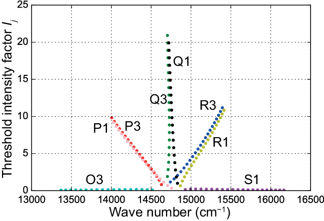
In Fig. S1 we show the values of $I_{j}$ obtained with Eq. (3) to (5) from Goldfarb et al. [3] and our Eqs. (S8,S9). As functions of the threshold energy $\tilde{\nu}_{j}$, the intensities are clearly grouped in branches. Their customary notation refers to the quantum number $N^{\prime}$ (total angular momentum except spin) of the respective dominant component (i.e., $N^{\prime}=J^{\prime}-1/2$ for F1 levels with $\Omega^{\prime}=3/2$ main component and $N^{\prime}=J^{\prime}+1/2$ for F2 levels). For a Q branch, $N^{\prime}=J^{\prime\prime}$, while branches R and P are defined by $N^{\prime}=J^{\prime\prime}\pm 1$ and S and O branches by $N^{\prime}=J^{\prime\prime}\pm 2$, respectively. Branches denoted as O3, P3, Q3 and R3 lead to F1 levels ($\Omega=3/2$ dominant), while the branches P1, Q1, R1 and S1 lead to F2 levels ($\Omega=1/2$ dominant). It is seen that, as expected, the P, Q and R branches of the F1 and F2 levels show similar behavior for high $J^{\prime\prime}$, while the O3 and S1 branches keep low amplitudes for all $J^{\prime\prime}$. This dramatically changes when the phases in Eqs. (S8,S9) are reversed.

The values of $I_{j}$ plotted in Fig. S1 show an approximately linear increase with $J^{\prime\prime}$. Hence, at excess photon energies $\tilde{\nu}-\tilde{\nu}_{0}$ large compared to the spacing between the rotational thresholds $\tilde{\nu}_{j}$, we will have a similar near-linear increase also for $I_{j}(\tilde{\nu}-\tilde{\nu}_{j})^{a}\approx I_{j}(\tilde{\nu}-\tilde{\nu}_{0})^{a}$. Only the division by the initial-state statistical weight, using the factors defined in Eq. (S1), avoids a drastic dependence on $J^{\prime\prime}$ of the cross section at high photon energies above the threshold. In previous applications [1, 3] the intensities $I_{j}$ were multiplied with pure Boltzmann factors (as opposed to level population fractions) in order to obtain the $J^{\prime\prime}$-dependent relative photodetachment intensities, which is consistent with our cross-section definition.

For another check, we have followed Schulz et al. [1] and reproduced their model of the electron spectra measured by Breyer et al. [7] for high excess photon energies (Fig. S2). It turned out that it is essential to apply the sign convention of Eqs. (S8,S9), together with a suitable cross-section definition, to obtain agreement with both the experimental and the earlier model data. The model results given in Ref. [1] can be reproduced accurately with the sign convention of Eqs. (S8,S9), which thus seems to be the one used by these authors (in spite of the opposite statement near Eq. (5) of Ref. [1]).

Molecules with infrared active modes like OH^- couple to the surrounding radiative field by emitting and absorbing photons. The rates of such processes can be described by the Einstein coefficients. We assume that the molecules are in the vibrational ground state only. Denoting in this section the OH^- quantum number by $J$, the level energies $\tilde{E}_{J}=\tilde{E}^{{\rm OH}^{-}}_{J^{\prime\prime}}$ are given by Eq. (S6) with $J^{\prime\prime}=J$ and the parameters from Table SI. Considering electric dipole transitions only, radiative transitions occur between adjacent $J$ levels only and we index the transition wave numbers by the lower $J$: $\tilde{\nu}_{J}=\tilde{E}_{J+1}-\tilde{E}_{J}$. The radiative field is specified by the photon occupation numbers at the transition frequencies, $n(\tilde{\nu}_{J})$, assuming the vacuum mode density and unpolarized conditions. If the radiation field can be characterized by a single temperature $T_{r}$, the photon occupation numbers follow the Bose-Einstein statistics,

with the Boltzmann constant $k_{B}$. By the rotational transitions, the radiative field is sampled at the approximately equidistant wave numbers $\tilde{\nu}_{J}\approx 2B_{0}(J+1)$.

The transition rates for radiative emission out of a level $J$ are given by

where $A_{J}$ is the Einstein coefficient for the spontaneous decay of level $J$:

from Ref. [8] assuming the Hönl-London factors [Eq. (9.115); Table 9.4 for R transitions]. Absorption processes out of $J$ have the rate

Together with the in-going processes into level $J$ the rate equation model is obtained:

We integrate the differential equation system with initial populations $p^{0}_{J}$ and close the system by setting $p_{J}\equiv 0$ and $A_{J}\equiv 0$ for $J>J_{\rm max}$ as well as for $J<0$. The used $p^{0}_{J}$ and, hence, $p_{J}$ are normalized ($\sum_{J}p_{J}=1$). Initial populations are defined by a Boltzmann distribution of temperature $T_{0}$. We work at $T_{0}<6\,000$ K and for this upper temperature limit, $p_{J}<10^{-4}$ for $J>50$. In the model we use $J_{\rm max}=50$.

The natural lifetimes $\tau_{J}=1/A_{J}$ decrease rapidly with $J$. As a consequence each excited rotational state cools faster than the next lower one. With the condition $\Delta J=\pm 1$ (R transitions, only) this slows down the radiative cascade into the rotational ground state. Moreover, the higher-$J$ states with shorter lifetime already thermalize among each other before population accumulates in the lower states. Approximately, the accumulation rate is limited by the lifetime of the lowest already thermalized level. This behavior significantly reduces the influence of the initial populations $p^{0}_{J}$ on those occuring after some in-vacuo relaxation time.

It should be noted that the decay constants of the $J$ levels are not in general identical to $A_{J}$, but modified by the ambient radiation field. In particular, the decay constant of the $J=1$ level, from finding the solution of Eq. (S14), amounts to $[1+4n(\tilde{\nu}_{J=0})]A_{1}$. Even at the present low-level cryogenic radiation field it is, thus, larger than $A_{1}$ by about 12% (see p. Radiation field at the lowest OH^- transition below).

The systematic uncertainties of the parameters from the fit of the probing signals are determined for various influences as follows.

Starting temperature. Fit results for the starting temperatures of 4000 K and 6000 K are compared, estimating the variations of the fit parameters for a starting temperature difference of $\pm 2000$ K around $T_{0}=6000$ K. This yields relative effects of $<0.1$% for $A_{1}$ and $A_{2}$ and of 0.15% for $A_{3}$, which are negligible w.r.t. the $1\sigma$ statistical uncertainties (1.3% for $A_{1}$ and 3% for $A_{2}$ and $A_{3}$). Similarly, the 0.03 K uncertainty of $T_{r}$ is neglected. For the fitted relative detachment cross sections, the uncertainties due to the starting temperature, determined by the same method, are linearly added to the $1\sigma$ statistical uncertainty to yield a total estimated uncertainty.

Rotational variation of the reference photodetachment cross section. The effect of a $J$-dependence in $\sigma_{r}$ at 15 754 cm^-1 can de estimated by considering the fit to $S_{4}$. At $t>150$ s, this essentially is determined by $J=1$ photodetachment only. For the final approach to equilibrium between $J=1$ and $J=0$, with relative populations at $t=150$ s of $p_{1}\approx p_{0}\approx 0.5$ at $t=150$ s, the signal $S_{4}\approx N_{J=1}(\tilde{\nu}_{4},t)/[N_{J=1}(\tilde{\nu}_{r},t)+N_{J=0}(\tilde{\nu}_{r},t)]$ can be modeled explicitly, introducing a relative cross section difference $\eta_{r}=\sigma_{r}^{J=1}/\sigma_{r}^{J=0}-1$. Fitting this model to the data using different near-zero values of $\eta_{r}$ yields a sensitivity of $\Delta A_{1}/\Delta\eta_{r}=+1.45\times 10^{-3}$ s^-1. We also searched for a component describing the $J=1$ decay in the reference signal $N(\tilde{\nu}_{r},t)$. This component has a decay rate of $[1+4n(\tilde{\nu}_{J=0})]A_{1}$ according to the radiative model. The search yields $\eta_{r}=-0.01(2)$. Hence, the systematic effect on $A_{1}$ due to the $J$-dependence of $\sigma_{r}$ is estimated as $\Delta A_{1}=-1.5(3.0)\times 10^{-5}$ s^-1. We choose to keep the value from the overall fit, $A_{1}=5.17(7)\times 10^{-3}$ s^-1, and linearly add a systematic uncertainty of $\pm 1$% due to the $J$-dependence of $\sigma_{r}$. The previous measurement in Ref. [9] indicates that the photodetachment cross section is independent of $J$ for $J=0$ to $2$ within $\sim$10%. Hence, for $J=2$ and $3$, we admit a $\sigma_{r}$ variation of $|\eta_{r}|<0.1$. Assuming the same relative effect of this variation on the Einstein coefficients, we estimate a systematic uncertainty of $\pm 3$% for $A_{2}$ and $A_{3}$, which is of similar order of magnitude as their statistical ones.

Differential laser depletion. Additional decays are expected in the normalized signals if photodetachment differently depletes the $J$-levels. An extreme upper limit for such effects is given by the observed decay constant $k_{0}=1.647(5)\times 10^{-3}$ s^-1 of the reference signal $N(\tilde{\nu}_{r},t)$. Considering the variation of $\sigma_{r}$ and the effect of the probing pulses at the various wave numbers, we estimate the differential laser depletion between $J=1$ and $J=0$ to represent $<0.03k_{0}\sim 5\times 10^{-5}$ s^-1, which introduces a relative uncertainty of $\sim$1% for $A_{1}$. A wider limit of $<0.1k_{0}\sim 2\times 10^{-4}$ s^-1 applies to $J\geq 2$, which again is of similar order of magnitude as the statistical uncertainties for these values.

Overall uncertainties. With $\sim$1% uncertainties for both the $J$-dependence of $\sigma_{r}$ and the differential laser depletion and a $1\sigma$ relative statistical uncertainty of 1.4%, we estimate the overall relative uncertainty of $A_{1}$ to 3.5%. For $A_{2}$ and $A_{3}$ the $1\sigma$ relative statistical uncertainties are 3.2% and 3.1%, respectively. Linearly adding the mentioned systematic uncertainty ranges, we estimate an overall relative uncertainty of 10% for $A_{2}$ and 7% for $A_{3}$.

Electric deflection fields. The 60-keV OH^- beam is deflected by electric fields $F$ up to 120 kV/m in the main CSR dipoles. This mixes a rotational state $|JM\rangle$ with neighboring levels $|J\pm 1\,M\rangle$ where the admixture ampitude is, from the coupling matrix element [10],

with $J_{>}=\max(J,J^{\prime})$. With $|E_{J}-E_{J^{\prime}}|\geq 2B$ ($B=2.32\times 10^{-3}$ eV) and $\mu\sim 1~\rm{D}$, the interaction energy is $\mu F\sim 2.5\times 10^{-6}$ eV and the admixture amplitude $|\varepsilon_{J^{\prime},J}^{M}|\lesssim 3\times 10^{-4}$. Squared matrix elements for additional decay channels opening up by this admixture will be smaller than those of allowed decay channels by a factor of $|\varepsilon_{J^{\prime},J}^{M}|^{2}\lesssim 1\times 10^{-7}$, which can be neglected. The steady-state admixed populations $|\varepsilon_{J^{\prime},J}^{M}|^{2}$ from different $J$ levels are also much smaller than the typical relevant $J$-level populations occurring in the present experiment.

In the relaxation and probing model, the Einstein $A$ coefficients from Eq. (S12) can either be fixed by giving the molecular dipole moment $\mu_{0}$ of OH^- or determined from the observed signal decays, as demonstrated in the main paper. In the latter case, each $A_{J}$ offers the option of extracting an effective molecular dipole moment $\mu_{0,J}$ (see Table I of the main paper). Considering the discussion of the ro-vibrational line strength $S_{J^{\prime}J^{\prime\prime}}$ in Bernath [8], p. 275f., using the Hönl-London factors and keeping the Herman–Wallis factor $F(m)$ [8] at 1 in the expression for $S_{J^{\prime}J^{\prime\prime}}$ [Eq. (7.229)], the value $\mu_{0}$ discussed in the main paper is equal to the vibrationally averaged dipole moment $M_{00}$, obtained with the vibrational wave functions for the $J=0$ molecule. We have modeled the OH^- vibrational wave function using a Morse potential and calculated the average of the calculated dipole moment function $\mu(R)$ [11] (see Fig. S3), which yields $\mu_{0}=M_{00}=1.037$ D. This is lower than the value at the equilibrium internuclear distance (Ref. [11], Table IV, MCFCF(5)-SCEP) by 0.035 and still deviates by 0.055 D or $\sim$5.3% from the measured value, $\mu_{0}=(0.982\pm 0.015)$ D. Using the calculated $\mu_{0}$, the rotational lifetimes are underestimated with respect to the measured values by $\sim$10%.. Calculating the wave function for $J=1$ including the centrifugal potential yields an estimated relative reduction of $\mu_{0}$ by the Herman–Wallis factor (assuming the same electronic potential for all $J$) of only $\sim$$2\times 10^{-4}$ for the $1\to 0$ transition.

In the experiment, we derive $T_{r}=15.1(1)$ K by sampling the radiation field on the transition $\tilde{\nu}_{J=0}=37.47$ cm^-1. The corresponding photon occupation number, from Eq. (S10), is $n(\tilde{\nu}_{J=0})=2.91(9)\times 10^{-2}=\bar{n}$. A plausible assumption is that the effective photon occupation number $\bar{n}$ seen by the stored OH^- ions reflects a linear superposition of effects from the CSR vacuum chambers at a temperature near 6 K [12] and from openings towards room-temperature surfaces (300 K). With a fractional room-temperature influence of $\epsilon$, the effective photon occupation number from this superposition would be $\bar{n}=\epsilon n_{300}+(1-\epsilon)n_{6}$. Table SII lists photon occupation numbers for the radiative temperatures of 6 K (close to the measured temperature of the CSR vacuum chambers) and for a 300 K environment. With these values, we find $\epsilon\sim\bar{n}/n_{300}=5.7(2)\times 10^{-3}$ for the fractional room-temperature influence. While it is difficult to estimate this value from the geometry, effective solid angles, reflection conditions, etc., this value is of the order of magnitude of the surface area that may be affected by room-temperature openings in the present arrangement of the CSR. In fact, a fraction of $\epsilon$ of the CSR circumference (35 m) amounts to $\sim$20 cm, of the order of the beam tube diameter.

In the data of Fig. 2 of the main paper, we find a background corresponding to a fraction of $(0.46\ldots 1.92)\times 10^{-2}$ of the rate at the reference $\tilde{\nu}_{r}$. Dividing by the laser-intensity normalization factor $S_{0}\sim 3$ (see the main paper), this yields for the photodetachment background a fractional size of $(0.13\ldots 0.45)\times 10^{-2}$ compared to the reference photodetachment rate. We assume this reference rate to be dominated by OH^-. If we explain the background through a contamination by ¹⁷O^-, the different photodetachment cross sections of OH^- and O^- must be considered. Taking Ref. [9] and the work cited therein, the O^- photodetachment cross section around 1.95 eV ($\sim$15 751 cm^-1) is smaller than that of OH^- at the same energy by a factor of $\sim$0.75, which yields a fractional abundance of ¹⁷O^- in the stored beam of $(1.7\ldots 5.9)\times 10^{-3}$. This value is plausible considering the ratio of the ¹⁶O^- and ¹⁶OH^- peaks found in mass spectra of the applied sputter ion source and the ¹⁷O^- natural abundance of $3.8\times 10^{-4}$ [13]. Variations of the value between runs can originate from changes of the ion source parameters. Moreover, the contaminating ¹⁷O^- may be partially suppressed by the dispersion of the mass selecting magnet in the injection beamline of the CSR and the amount of the suppresion can vary with the precise tuning of the injection beam line.

For reference we give the probing wave numbers $\tilde{\nu}_{k}$ and the experimental photodetachment cross-section ratios for OH^- from this work, together with the model results (Table SIII). The measured ratios are precise enough ($\sim$3 to 16%) to serve as experimentally derived probing sensitivities and may be used to derive rotational population fractions from comparing photodetachment rates at specific probing wave numbers $\tilde{\nu}_{k}$.

References

- [1] P. A. Schulz, R. D. Mead, and W. C. Lineberger, Phys. Rev. A 27, 2229 (1983).
- [2] J. D. Rudmin, L. P. Ratliff, J. N. Yukich, and D. J. Larson, J. Phys. B: At. Mol. Opt. Phys. 29, L881 (1996).
- [3] F. Goldfarb, C. Drag, W. Chaibi, S. Kröger, C. Blondel, and C. Delsart, J. Chem. Phys. 122 (2005), 10.1063/1.1824904.
- [4] J. P. Maillard, J. Chauville, and A. W. Mantz, J. Mol. Spectrosc. 63, 120 (1976).
- [5] P. A. Schulz, R. D. Mead, P. L. Jones, and W. C. Lineberger, J. Chem. Phys. 77, 1153 (1982).
- [6] S. Gewurtz, H. Lew, and P. Flainek, Can. J. Phys. 53, 1097 (1975).
- [7] F. Breyer, P. Frey, and H. Hotop, Z. Phys. A 300, 7 (1981).
- [8] P. F. Bernath, Spectra of Atoms and Molecules, 2nd ed. (Oxford University Press, New York, 2005).
- [9] P. Hlavenka, R. Otto, S. Trippel, J. Mikosch, M. Weidemüller, and R. Wester, J. Chem. Phys. 130, 061105 (2009).
- [10] Y.-P. Chang, F. Filsinger, B. G. Sartakov, and J. Küpper, Comp. Phys. Commun. 185, 339 (2014).
- [11] H. Werner, P. Rosmus, and E. Reinsch, J. Chem. Phys. 79, 905 (1983).
- [12] R. von Hahn, A. Becker, F. Berg, K. Blaum, C. Breitenfeldt, H. Fadil, F. Fellenberger, M. Froese, S. George, J. Göck, M. Grieser, F. Grussie, E. A. Guerin, O. Heber, P. Herwig, J. Karthein, C. Krantz, H. Kreckel, M. Lange, F. Laux, S. Lohmann, S. Menk, C. Meyer, P. M. Mishra, O. Novotný, A. P. O’Connor, D. A. Orlov, M. L. Rappaport, R. Repnow, S. Saurabh, S. Schippers, C. D. Schröter, D. Schwalm, L. Schweikhard, T. Sieber, A. Shornikov, K. Spruck, S. Sunil Kumar, J. Ullrich, X. Urbain, S. Vogel, P. Wilhelm, A. Wolf, and D. Zajfman, Rev. Sci. Instrum. 87, 063115 (2016).
- [13] G. L. Molnár and R. B. Firestone, in Handbook of Nuclear Chemistry, edited by A. Vértes, S. Nagy, Z. Klencsár, R. G. Lovas, and F. Rösch (Springer US, 2011) pp. 475–610.