Dynamics of modular matings

An $(m:n)$ holomorphic correspondence on the Riemann sphere $\widehat{\mathbb{C}}$ is an $n$-valued function $F:z\to w$ (with $m$-valued inverse $F^{-1}:w\to z$) defined implicitly by a polynomial equation $P(z,w)=0$, where $P$ has degree $m$ in $z$ and $n$ in $w$. In this paper we study the dynamics under iteration of members of a particular one complex parameter family of $(2:2)$ holomorphic correspondences, namely the family ${\mathcal{F}}_{a}:z\to w$, given by

$$\left(\frac{az+1}{z+1}\right)^{2}+\left(\frac{az+1}{z+1}\right)\left(\frac{aw-1}{w-1}\right)+\left(\frac{aw-1}{w-1}\right)^{2}=3,$$

introduced by the first author, together with Christopher Penrose, in [BP]. For this family, there exists an open set $\mathcal{K}\subset\mathbb{C}$, called the Klein Combination Locus, such that for all $a\in\mathcal{K}$ the Riemann sphere admits a partition into two subsets completely invariant under $\mathcal{F}_{a}$, denoted $\Lambda_{a}$ and $\Omega_{a}$. The limit set $\Lambda_{a}$ is closed and is the union of two closed subsets, the forwards limit set $\Lambda_{a,-}$, restricted to which $\mathcal{F}_{a}$ is $(2:1)$, and the backwards limit set $\Lambda_{a,+}$, on which $\mathcal{F}_{a}$ is $(1:2)$; the intersection $\Lambda_{a,-}\cap\Lambda_{a,+}$ consists of a parabolic fixed point of $\mathcal{F}_{a}$ of multiplier $1$ (see Section 2). The complement $\Omega_{a}={\widehat{\mathbb{C}}}\setminus\Lambda_{a}$ of the limit set is called the regular set. The connectedness locus $\mathcal{C}_{\Gamma}$ for the family $\mathcal{F}_{a}$ is the set of $a\in\mathbb{C}$ such that the limit set $\Lambda_{a}$ is connected (see Section 2). In [BL1], the current authors prove that when $a\in\mathcal{C}_{\Gamma}$ the correspondence $\mathcal{F}_{a}$ behaves like a parabolic quadratic map of the form

$$P_{A}(z)=z+1/z+A$$

on a doubly pinched neighbourhood of $\Lambda_{a,-}$, using parabolic-like maps (see [L]), and like the modular group on its complement. To make the statement precise, let us recall that, for every $A\in\mathbb{C}$, the map $P_{A}$ has a parabolic fixed point at $z=\infty$ with multiplier $1$, and basin of attraction $\mathcal{A}_{A}(\infty)$; the filled Julia set $K_{A}$ of $P_{A}$ is defined to be $K_{A}=\widehat{\mathbb{C}}\setminus\mathcal{A}_{A}(\infty)$. The Main Theorem in [BL1] states that for every $a\in\mathcal{C}_{\Gamma}$, the correspondence $\mathcal{F}_{a}$ is hybrid conjugate on a doubly pinched neighbourhood of $\Lambda_{a,-}$ to a rational map of the form $P_{A}$ acting on a doubly pinched neighbourhood of its filled Julia set $K_{A}$, and on its regular set $\Omega_{a}$ the correspondence $\mathcal{F}_{a}$ is conformally conjugate to the pair of generators

$$\alpha:z\to z+1\ \ \ \ {\rm and}\ \ \ \ \beta:z\to\frac{z}{z+1}$$

of the modular group $\Gamma=PSL(2,\mathbb{Z})$ acting on the complex upper half-plane $\mathbb{H}$. In other words, for every $a\in{\mathcal{C}}_{\Gamma}$ the correspondence ${\mathcal{F}}_{a}$ is a mating between a rational map of the form $P_{A}:z\to z+1/z+A$ and $\Gamma$. In view of this theorem, we call the correspondences in the family $\mathcal{F}_{a}$ modular matings. We define the modular Mandelbrot set $\mathcal{M}_{\Gamma}$ to be $\mathcal{M}_{\Gamma}:=\mathcal{C}_{\Gamma}\cap\overline{\mathbb{D}}(4,3)$. See Figure 3.

In the current paper we develop a complete dynamical theory for these modular matings. For a general holomorphic correspondence on the Riemann sphere, analysing dynamics under iteration is a very challenging problem, even in the $(2:2)$ case. It is akin to the problem of analysing the dynamics of the group generated by a general pair of fractional linear transformations, and it is well known that for such a group it is a non-trivial problem even to determine whether it is discrete. Isolated examples of correspondences (for example the arithmetic-geometric mean) are well understood. The family of correspondences $\mathcal{F}_{a},a\in\mathcal{M}_{\Gamma}$, is the simplest $1$-parameter family to be fully explored, and as such it should provide a paradigm for the study of other families of correspondences displaying “discreteness” in their action on the sphere for some subset of parameter space.

For $a\in{\mathcal{C}}_{\Gamma}$, the Main Theorem in [BL1] guarantees the existence of a canonical conformal homeomorphism

$$\varphi_{a}:\widehat{\mathbb{C}}\setminus\Lambda({\mathcal{F}}_{a})\to{\mathbb{H}},$$

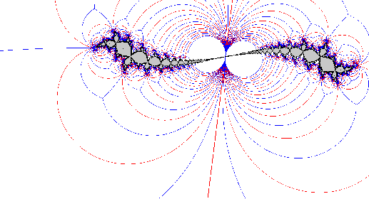
conjugating the correspondence restricted to $\Omega({\mathcal{F}}_{a})$ to the pair of generators $\alpha,\beta$ of the modular group defined above (see Figure 1 and Section 3). We call this map the Böttcher map for the correspondence ${\mathcal{F}}_{a}$, $a\in{\mathcal{C}}_{\Gamma}$, because it plays a role in our theory analogous to that of the classical Böttcher map

$$\varphi_{c}:\widehat{\mathbb{C}}\setminus K(Q_{c})\to\widehat{\mathbb{C}}\setminus\overline{\mathbb{D}}$$

which conjugates a quadratic polynomial $Q_{c}:z\to z^{2}+c$ on the complement of its filled Julia set $K(Q_{c})$ to the map $z\to z^{2}$ on the complement of the closed unit disc, whenever $c$ lies in the Mandelbrot set ${\mathcal{M}}$, the set of $c\in\mathbb{C}$ such that $K_{c}$ is connected. Let us recall that external rays are the lines $R_{\theta}=\{z|\arg(\varphi_{c}(z))=\theta\}$, preimages under the Böttcher map $\varphi_{c}$ of lines of constant argument in $\mathbb{C}$, and are important tools to understand the dynamics of a polynomial. Douady and Hubbard proved that periodic rays land (that is, there exists a limit, necessarily in $\partial K(Q_{c})$, for $\varphi_{c}^{-1}(re^{2\pi i\theta})$ as $r\to 1$), and that repelling periodic points are landing points of at least one and at most finitely many external rays. By considering properties of the linearisation of $Q_{c}$ in the neighbourhood of a repelling periodic cycle, Yoccoz proved, for $Q_{c}$ with $c\in{\mathcal{M}}$, an inequality constraining the (complex) logarithm of the multiplier of a repelling periodic cycle to lie in a certain disc in $\mathbb{C}$ (see [H] and Figure 2), an inequality which he applied to estimate the size of the limbs of the Mandelbrot set.

There are strong parallels between the dynamical theories for the family $\mathcal{F}_{a}$ and the family $Q_{c}$, but also essential differences. The core similarity is that both theories are constructed using isometries of the hyperbolic metric on $\mathbb{H}$: the map $z\to z^{2}$ on the punctured disc $\mathbb{C}\setminus\overline{\mathbb{D}}$ lifts to the isometry $z\to 2z$ on its universal cover $\mathbb{H}$, and external rays in $\mathbb{C}\setminus K(Q_{c})$ are the preimages, under the lift of the Böttcher map, of geodesics in $\mathbb{H}$ from points of $\mathbb{R}\subset\partial\mathbb{H}$ to $\infty$. The core difference between the theories comes from fact that $z\to 2z$ is a hyperbolic isometry (it has two fixed points, $0$ and $\infty$ on $\partial\mathbb{H}$), whereas $z\to\alpha(z)$ and $z\to\beta(z$) are two parabolic isometries (with one fixed point each, $\infty$ and $0$, respectively). The modular group endows ${\mathbb{H}}$ with a richer structure than that which the angle-doubling map gives to $\widehat{\mathbb{C}}\setminus\overline{\mathbb{D}}$, but conversely there is no single point in ${\mathbb{H}}$ which has properties for $\Gamma$ analogous to those enjoyed by $\infty\in\widehat{\mathbb{C}}\setminus\overline{\mathbb{D}}$ for the angle-doubling map. For the family $\mathcal{F}_{a}$ the role of external rays in the Douady-Hubbard theory for $Q_{c}$ is replaced by that of geodesics in $\widehat{\mathbb{C}}\setminus\Lambda_{a}$ with initial point in $\Lambda_{a,-}$ and final point in $\Lambda_{a,+}$. The Douady-Hubbard theory makes frequent use of a Green’s function $G_{c}:{\mathbb{C}}\setminus K(Q_{c})\to{\mathbb{R}}^{>0}$ which interacts with the dynamics via $G_{c}(Q_{c}(z))=2G_{c}(z)$. The Green’s function $G_{a}$ for $\Lambda_{a}$ has no such simple relationship with the two branches of $\mathcal{F}_{a}$, but for points close to $\Lambda_{a,-}$ we prove that there exist lower and upper bounds for the multiplying factor $G_{a}(\mathcal{F}_{a}(z))/G_{a}(z)$ (Lemma 2, Section 3.2). This weaker property suffices for our purposes.

In Proposition 1 (Section 3) we prove that the inverse $\psi_{a}$ of the Böttcher map extends continuously to the end points of the imaginary axis ${\mathcal{I}}$ in ${\mathbb{H}}$ (the geodesic running from $0$ to $\infty$) sending both $0$ and $\infty$ to the parabolic fixed point $\Lambda_{a,-}\cap\Lambda_{a,+}$ (see Fig. 1), in other words that this geodesic lands, at both ends. In Proposition 2 (Section 4) we prove that periodic geodesics land. Here, by a periodic geodesic we mean one which is mapped to itself by some finite sequence of branches of $\mathcal{F}_{a}$: under the Böttcher map $\varphi_{a}$ it corresponds to a geodesic in ${\mathbb{H}}$ fixed by some finite product of positive powers of $\alpha$ and $\beta$. (Note that while ${\mathcal{I}}$ is not itself a periodic geodesic, its end-points are fixed by $\alpha$ and $\beta$ respectively.) We then explain how one may code a geodesic in $\mathbb{H}$ from a point in $\mathbb{R}^{-}$ to a point in $\mathbb{R}^{+}$ by a bi-infinite sequence $S\in\{\alpha,\beta\}^{\mathbb{Z}}$ combining the continued fraction expansions of these two points. The $2$-sided shift operator on bi-infinite sequences imposes a dynamic on the space of geodesics from $\mathbb{R}^{-}$ to $\mathbb{R}^{+}$ in which the periodic geodesics play an organising role. By adapting a technique due to Benini and Lyubich [BeLy], in Section 5 we prove the deeper converse to Proposition 2 that repelling periodic points are landing points of periodic geodesics. More precisely:

As a consequence of Theorem 1(i), we may define the combinatorial rotation number of a repelling fixed point $\hat{z}$ of $f_{a}$ (where $a\in{\mathcal{C}}_{\Gamma}$) to be the rotation number of the unique periodic cycle of geodesics landing at $\hat{z}$. In Section 6 we prove an inequality of Pommerenke-Levin-Yoccoz type for our correspondences at such a fixed point:

In the original Yoccoz inequality for quadratic polynomials, the corresponding radius $r_{p/q}$ is $1/q$ [H]. Writing $2\pi i\nu$ for the imaginary part of $\log{\zeta}$, we deduce that whereas in the classical Yoccoz case for $c$ to be in $\mathcal{M}$ the value of $\log{\zeta}$ (where $\zeta$ is the derivative of $Q_{c}$ at a repelling fixed point) must lie in a strip whose width goes to zero linearly with $\nu$, in our situation for $a$ to be in $\mathcal{M}_{\Gamma}$ the value of $\log{\zeta}$ has to lie in a strip whose width goes to zero at a rate proportional to $\nu^{2}\log(1/\nu)$ (for $\nu=1/q$ this is $(\log{q})/q^{2}$): see Figure 2. For repelling orbits of period greater than $1$ the bound on the modulus of the derivative is more complicated: see Remark 4 at the end of Section 6 for an example.

In Section 7 we apply Theorem 2 to prove that the modular Mandelbrot set $\mathcal{M}_{\Gamma}$ is contained in a subset of $\mathbb{C}$ of a particular form. By the lune ${\mathcal{L}}_{\theta}$ in the parameter plane we shall mean the closed subset of the $a$-plane bounded by the two arcs of circles which pass through the points $a=1$ and $a=7$ and meet the real axis at angles $\pm\theta$ at these points (so the lune ${\mathcal{L}}_{\pi/2}$ is the disc $\overline{\mathbb{D}}(4,3)$). The plot on the right in Figure 3 suggests the possibility that ${\mathcal{M}}_{\Gamma}\subset{\mathcal{L}}_{\pi/3}$. We do not know if this is the case, but we prove:

Writing $L_{p/q}$ for the $p/q$-limb of $\mathcal{M}_{\Gamma}$, the set of parameter values where the fixed point of $\mathcal{F}_{a}$ is repelling or neutral of combinatorial rotation number $p/q$, and writing $a_{p/q}$ for the root point of $L_{p/q}$, the value of $a$ where the derivative of $\mathcal{F}_{a}$ at its fixed point is $e^{2\pi ip/q}$, the computations in the proof of Theorem 3 specialise to:

Indeed the picture in the $a$-plane close to $a=7$ is the image of the lefthand plot in Figure 2 under the transformation $\log{\zeta}\to 7+6(i\log{\zeta})^{2/3}$.

For the convenience of the reader, Table 1 exhibits parallels between the Douady-Hubbard theory for quadratic polynomials $Q_{c}$ and the theory developed below for the quadratic correspondences ${\mathcal{F}}_{a}$.

In a sequel [BL3] to the present paper we shall show that when $a$ lies in the parameter space lune ${\mathcal{L}}_{\theta}$ established by Theorem 3, we may choose a dynamical space lune $L_{a}$, depending analytically on $a$, on which to perform a surgery to transform the correspondence ${\mathcal{F}}_{a}$ into a rational map of the form $z\to z+1/z+A$, that is to say a quadratic rational map whose conjugacy class lies in Milnor’s slice $Per_{1}(1)$. Then, using the theory of holomorphic motions we shall prove the following conjecture, in which $\mathcal{M}_{1}$ denotes the connectedness locus of the family $Per_{1}(1)$:

In [PR] Carsten Petersen and Pascale Roesch prove that $\mathcal{M}_{1}$ is homeomorphic to the classical Mandelbrot set $\mathcal{M}$. Thus proving Conjecture 1 will yield a mathematical justification of the resemblance between $\mathcal{M}_{\Gamma}$ and $\mathcal{M}$ first noted experimentally almost three decades ago in [BP].

The anti-holomorphic case. Contemporaneously with our work, but independently of it, Lee, Lyubich, Makarov and Mukherjee [LLMM] investigated matings between quadratic anti-rational maps and a discrete group generated by hyperbolic reflections, as part of their innovative programme of study of the dynamics of Schwarz reflection maps associated to quadrature domains. Their notion of a mating between a map and a group differs from ours, in that theirs is a single-valued function, which on an invariant closed connected subset has the behaviour of an anti-rational map on its filled Julia set, and which on the complement is associated to a discrete group of isometries of $\mathbb{H}$ generated by a reflection and a rotation. Despite the differences, there is a close relationship between the two settings. The dynamics of an (anti-holomorphic) Schwarz reflection maps in the one parameter family considered in [LLMM] strongly parallels that of a $(2:1)$ restriction of a holomorphic correspondence in the one parameter family investigated in [BP], [BL1], and the present paper. See Remark 1 at the end of Section 2, where the relationship between the two theories is elucidated.

Acknowledgement. This work was supported by the Serrapilheira Institute (grant number Serra-1811-26166), the EU Marie-Curie IRSES Brazilian-European partnership in Dynamical Systems (FP7-PEOPLE-2012-IRSES 318999 BREUDS), the Fundação de amparo a pesquisa do estado de São Paulo (Fapesp, process 2013/20480-7), the Cnpq (406575/2016-19), and the prize L’ORÉAL-UNESCO-ABC Para Mulheres na Ciência.

In this Section we note some general definitions and properties of $(2:2)$ holomorphic correspondences, and recall terminology and results from [BL1], which we shall use throughout the paper.

A $(2:2)$ holomorphic correspondence on the Riemann sphere is a $2$-valued function $F:z\to w$ (with $2$-valued inverse $F^{-1}:w\to z$) defined implicitly by a polynomial equation $P(z,w)=0$, where $P$ has the form

$$P(z,w)=(az^{2}+bz+c)w^{2}+(dz^{2}+ez+f)w+(gz^{2}+hz+j).$$

The graph of $F$, the Riemann surface $P(z,w)=0$, supports two natural involutions: $I_{-}$ which interchanges the two values of $z$ which map to the same $w$, and $I_{+}$ which interchanges the two values of $w$ which are images of the same $z$. We say that $F$ is a map of triples if $(I_{+}I_{-})^{3}$ is the identity. Equivalently the immediate images $w_{2},w_{3}$ of any point $z_{1}$, and the immediate pre-images of $w_{2}$ and $w_{3}$ fit together in a closed diagram:

which at isolated points may take one of the degenerate forms below:

In the diagram on the left, $(z_{2},w_{1})$ is a fixed point of $I_{-}$ and $(z_{1},w_{2})$ is a fixed point of $I_{+}$. We remark that $dw/dz=0$ for the forwards branch $z_{2}\to w_{1}$, and $dz/dw=0$ for the backwards branch $w_{2}\to z_{1}$; thus the four points in the diagram are all forwards or backwards critical points or values of the correspondence. In the diagram on the right, $(z_{1},w_{1})$ is fixed by both $I_{-}$ and $I_{+}$; the point $(z_{1},w_{1})$ is a double point of the Riemann surface $P(z,w)=0$.

It follows from the definition, or equivalently from the diagrams above, that every map of triples necessarily factorises into the deleted covering correspondence $Cov_{0}^{C}$ of a cubic $C:\widehat{\mathbb{C}}\to\widehat{\mathbb{C}}$ post-composed by a Möbius transformation $M$. Here $C$ is the map which identifies each triple of points $\{z_{1},z_{2},z_{3}\}$ of the diagram condition to a single point, and $M$ is the map which sends each $z_{j}$ in the diagram to the corresponding $w_{j}$. Up to pre- and post-multiplication by Möbius transformations, $C$ can take one of three forms, depending on the numbers and types of critical points of the correspondence:

1. (i)

   $C(z)=z^{3}$;

2. (ii)

   $C(z)=z^{3}-3z$;

3. (iii)

   $C(z)=z^{2}(z+a)/(z+1)\ (a\neq 0,1,9)$.

These forms correspond to the three possible topological types for the graph of a $(2:2)$ holomorphic correspondence, namely two (intersecting) spheres, a single (self-intersecting) sphere, or (the generic case) an elliptic curve. Our interest is in the second case, and the particular sub-case that the Möbius transformation $M$ is an involution (which we denote $J$). This restriction reduces us to the two (complex) parameter family of reversible maps of triples which have graph a single sphere. Our final restriction, reducing us to one parameter, is to require that one of the fixed points of $J$ be also a critical point of $Cov_{0}^{C}$. Hence, we can write $\mathcal{F}_{a}=J_{a}\circ Cov_{0}^{C}$, where $Cov^{C}_{0}$ denotes the deleted covering correspondence of $C(z)=z^{3}-3z$, that is to say the $2$-to-$2$ correspondence $Z\to W$ on $\widehat{\mathbb{C}}$ defined by

$$\frac{C(Z)-C(W)}{Z-W}=0,\quad{\rm that\ is,}\quad Z^{2}+ZW+W^{2}=3,$$

and $J_{a}$ denotes the conformal involution on $\widehat{\mathbb{C}}$ which has fixed points $Z=1$ and $Z=a$, namely

$$J_{a}(Z)=\frac{(a+1)Z-2a}{2Z-(a+1)}.$$

Thus the correspondence $\mathcal{F}_{a}:Z\rightarrow W$ is given by

$$Z^{2}+ZJ(W)+(J(W))^{2}=3,$$

which under the change of coordinates

$$Z=(az+1)/(z+1),\mbox{ and }W=(aw+1)/(w+1)$$

is the relation

$$\left(\frac{az+1}{z+1}\right)^{2}+\left(\frac{az+1}{z+1}\right)\left(\frac{aw-1}{w-1}\right)+\left(\frac{aw-1}{w-1}\right)^{2}=3.$$

By construction, the involution $J_{a}$ conjugates ${\mathcal{F}}_{a}$ to its inverse ${\mathcal{F}}_{a}^{-1}$. In the $z$-coordinate $J$ is the involution $z\to-z$ (whatever the value of $a$). The forwards critical points of ${\mathcal{F}}_{a}$ (the points where $dW/dZ$ vanishes for a branch $Z\to W$ of ${\mathcal{F}}_{a}$, see [BP] Section 2) are $Z=-1$ and $+1$. The corresponding forwards critical values are $W=J(+2)$ and $J(-2)$ respectively. The point $Z=\infty$ is a double point of ${\mathcal{F}_{a}}$ (see [BP] Section 2).

As $\mathcal{F}_{a}=J_{a}\circ Cov_{0}^{C}$, the two images of $Z\in\mathbb{C}$ under $\mathcal{F}_{a}$ are the images under $J_{a}$ of the two preimages of $C(Z)=Z^{3}-3Z$ in $\mathbb{C}$ different from $Z$. Using this decomposition, we will now construct fundamental domains for the action of $\mathcal{F}_{a}$. As $Z=1$ is a critical point of the cubic $C$, and $C(-2)=C(1)$, we deduce that $Cov_{0}^{C}(-2)=1$ under both branches, and $Cov_{0}^{C}((-\infty,-2])$ is a smooth curve running through $Z=1$, symmetric about the real axis, and asymptotic to the directions $e^{\pm\pi i/3}$ as $Z$ tends to $\infty$. On the other hand, $J_{a}$ fixes the circle through $Z=1$ and $Z=a$ having centre on the real axis, and sends points inside the disc bounded by this circle to the exterior of the disc, and vice versa. The standard fundamental domain $\Delta^{st}_{Cov}$ is the subset of the $Z$-plane to the right of the curve $Cov_{0}^{C}((-\infty,-2])$. The standard fundamental domain $\Delta^{st}_{J}$ is the subset of the $Z$-plane exterior to the circle through $Z=1$ and $Z=a$ which has centre on the real axis (see Figure 4 on the left). Define $\mathcal{D}:=\{a:|a-4|\leq 3\}$, and note that for $a=1$ the correspondence is not defined. When $a\in\mathcal{D}\setminus\{1\}$, we have

$$\Delta^{st}_{Cov}\cup\Delta^{st}_{J}=\widehat{\mathbb{C}}\setminus\{1\}.$$

Moreover, when $|a-4|<3$ these satisfy the condition that their boundaries are transverse to the parabolic axis at $Z=1$ (see Proposition 3.5 in [BL1] for a proof). When $a=7$ there are three attracting-repelling directions at $Z=1$ and the domain boundaries are transverse to all three.

More generally, the Klein Combination Locus, $\mathcal{K}$, is the set of values of the parameter $a\in\widehat{\mathbb{C}}$ such that there exist fundamental domains $\Delta_{Cov}$ for $Cov_{0}^{C}$ and $\Delta_{J}$ for $J$ which together cover all of $\widehat{\mathbb{C}}$ except for the single point $Z=1$ ($z=0$) (in the present article, as in [BL1], fundamental domains are open, so do not include their boundaries). A pair of fundamental domains $(\Delta_{Cov},\Delta_{J})$ satisfying this condition is called a Klein combination pair. Since the standard fundamental domains are a Klein combination pair, we have that $\mathcal{D}\setminus\{1\}\subset\mathcal{K}$. When $a\in{\mathcal{K}}$ we can always choose $\Delta_{Cov}$ and $\Delta_{J}$ such that the Jordan curves $\partial\Delta_{Cov}$ and $\partial\Delta_{J}$ are smooth at the parabolic fixed point $Z=1$ ($z=0$) of ${\mathcal{F}}_{a}$, and transverse to the attracting-repelling axis there (see Proposition 3.8 in [BL1]).

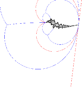
By construction, when $a\in{\mathcal{K}}$ and $(\Delta_{Cov},\Delta_{J})$ is a Klein combination pair, ${\mathcal{F}}_{a}$ restricted to the domain $\Delta_{Cov}$ is a $1$-to-$2$ correspondence (see Figure 4 on the right, and Proposition 3.4 in [BL1] for a proof):

$${\mathcal{F}}_{a}:\Delta_{Cov}\to J(\widehat{\mathbb{C}}\setminus\Delta_{Cov})\subset\Delta_{Cov}.$$

Provided that $\Delta_{Cov}$ and $\Delta_{J}$ have smooth boundaries at the parabolic point and that these are transverse to the attracting-repelling axis there,

$$\Lambda_{a,+}:=\bigcap_{n=0}^{\infty}{\mathcal{F}}_{a}^{n}(\Delta_{Cov})$$

is independent of the choice of the Klein combination pair $(\Delta_{Cov},\Delta_{J})$. We call $\Lambda_{a,+}$ the forwards limit set of ${\mathcal{F}}_{a}$. Moreover, $\widehat{\mathbb{C}}\setminus\Delta_{Cov}\subset J(\Delta_{Cov})$ and the restriction of ${\mathcal{F}}_{a}$ is a $2$-to-$1$ map from the first of these sets onto the second. We define the backwards limit set of ${\mathcal{F}}_{a}$ (see Figure 5) to be

$$\Lambda_{a,-}:=\bigcap_{n=0}^{\infty}{\mathcal{F}}_{a}^{-n}(\widehat{\mathbb{C}}\setminus\Delta_{Cov}).$$

Also by construction, $\Lambda_{a,-}=J(\Lambda_{a,+})$ and $\Lambda_{a,-}\cap\Lambda_{a,+}$ consists of a single point, the parabolic fixed point ($Z=1$) of ${\mathcal{F}}_{a}$. We denote $\Lambda_{a,-}\cup\Lambda_{a,+}$ by $\Lambda_{a}$. Finally, ${\mathcal{F}}_{a}$ acts properly discontinuously on $\Omega_{a}=\widehat{\mathbb{C}}\setminus\Lambda_{a}$, with fundamental domain $\Delta_{corr}:=\Delta_{Cov}\cap\Delta_{J}$.

Further restricting the codomain of the $2$-to-$1$ branch of ${\mathcal{F}}_{a}$ defined above to $\overline{\Delta}_{J}$, yields a $2$-to-$1$ map which we denote $f_{a}$. This inherits the property that $f_{a}^{-1}(\overline{\Delta}_{J})\subset\overline{\Delta}_{J}$. Modulo boundary curves, $\overline{\Delta}_{J}\setminus f_{a}^{-1}(\overline{\Delta}_{J})$ is the disjoint union of $\Delta_{Cov}\cap\Delta_{J}$ and its two images under $Cov_{0}^{C}$. The map $f_{a}$ has unique critical point $Z=-1$ in $\Delta_{J}$ (the other forwards critical point $Z=+1$ of ${\mathcal{F}}_{a}$ being a fixed point on the boundary $\partial\Delta_{J}$).

The connectedness locus ${\mathcal{C}}_{\Gamma}$ is the set of parameter values $a\in{\mathcal{K}}$ such that $\Lambda_{a,-}$ (or equivalently $\Lambda_{a,+}$ or $\Lambda_{a}$) is connected. The modular Mandelbrot set, $\mathcal{M}_{\Gamma}$, is ${\mathcal{C}}_{\Gamma}\cap\mathcal{D}$. It is proved in [BL3] that $\mathcal{M}_{\Gamma}={\mathcal{C}}_{\Gamma}$.

By Theorem A of [BL1], for every $a\in\mathcal{C}_{\Gamma}$ there exists a conformal homeomorphism $\varphi_{a}:\Omega_{a}\to{\mathbb{H}}$ which conjugates the two branches of ${\mathcal{F}}_{a}|_{\Omega_{a}}$ to the automorphisms $\alpha:z\to z+1$ and $\beta:z\to z/(z+1)$ of ${\mathbb{H}}$. This $\varphi_{a}$ is unique, since any automorphism $h$ of ${\mathbb{H}}$ which conjugates both $\alpha$ to itself and $\beta$ to itself is necessarily the identity (to see this, observe that $h$ must fix both $\infty$ and $0$, and that therefore $h$ has the form $h(z)=\lambda z$; the fact that $h^{-1}\alpha h(z)=\alpha(z)$ for all $z\in{\mathbb{H}}$ now implies that $\lambda=1$). We shall refer to $\varphi_{a}$ as the ‘Böttcher map’. It is analogous to the map:

$$\varphi_{c}:{\mathbb{C}}\setminus K(Q_{c})\to{\mathbb{C}}\setminus\overline{\mathbb{D}}$$

defined by Douady and Hubbard [DH], from the complement of the filled Julia set $K(Q_{c})$ of a quadratic polynomial $Q_{c}(z)=z^{2}+c$ (with $c\in\mathcal{M}$) to the complement of the closed unit disc, conjugating $Q_{c}$ to $z\to z^{2}$.

Notation. For $a\in{\mathcal{C}}_{\Gamma}$, the two branches of the correspondence ${\mathcal{F}}_{a}$ become (single-valued) homeomorphisms when we restrict ${\mathcal{F}}_{a}$ to $\Omega=\Omega({\mathcal{F}}_{a})$. We denote these homeomorphisms by $g:\Omega\to\Omega$ and $h:\Omega\to\Omega$, where $g$ corresponds under $\varphi_{a}$ to $\alpha$, and $h$ corresponds to $\beta$.

We recall that $PSL(2,{\mathbb{Z}})$ is the free product of the subgroups $C_{2}$ generated by $\sigma:z\to-1/z$ and $C_{3}$ generated by $\rho:z\to-1-1/z$. Under the Böttcher map $\varphi_{a}$ the branch $g$ of ${\mathcal{F}}_{a}|_{\Omega_{a}}$ corresponds to $\sigma\rho$ and $h$ corresponds to $\sigma\rho^{-1}$. Thus $g^{-1}hg^{-1}$ corresponds to $\sigma$ and $g^{-1}h$ corresponds to $\rho$. We deduce:

Pursuing the same route as that followed by Douady and Hubbard for polynomials, we now consider the question as to how far the inverse of $\varphi_{a}$ extends to a continuous map from the boundary of ${\mathbb{H}}$ to the boundary of $\Omega=\Omega({\mathcal{F}}_{a})$.

Proof Let $\mathcal{I}$ denote the imaginary axis in ${\mathbb{H}}$, the geodesic which runs from $0\in\partial{\mathbb{H}}$ to $\infty\in\partial{\mathbb{H}}$. The homeomorphism $\psi_{a}:{\mathbb{H}}\to\Omega$ sends $\mathcal{I}$ and its images under the cyclic group generated by $\alpha:{\mathbb{H}}\to{\mathbb{H}}$ to an arc $\psi(\mathcal{I})$ in $\Omega$ and its images under the cyclic group generated by $g:\Omega\to\Omega$. The points $it\in\mathcal{I}$, $t\to\infty$, lie on horocycles of $\alpha$ in a family converging to the fixed point $z=\infty$ of $\alpha$, on the boundary of ${\mathbb{H}}$. So their images $\psi_{a}(it)$, $t\to\infty$, lie on horocycles of $g$ in a family which converges to the fixed point $Z=1$ of $g$ (see Step 3 in the proof of Theorem A in [BL1]). Thus the boundary point $Z=1$ is accessible from within $\Omega$ by the path $\psi_{a}(\mathcal{I})$, and setting $\psi_{a}(\infty)=1$ therefore extends $\psi_{a}$ continuously to the end point $z=\infty$ of $\mathcal{I}$. The proof for the other end of $\mathcal{I}$ is similar, with $\beta$ in place of $\alpha$ and $h$ in place of $g$. ∎

Proof This follows immediately from Proposition 1, since the orbit of $0\in{\mathbb{R}}$ under $PSL(2,{\mathbb{Z}})$ is ${\mathbb{Q}}$. ∎

We remark that the rationals perform the same role here as that of the dyadic rationals (those with finite binary expressions) in the case of quadratic polynomials. In Subsection 4.1 the quadratic irrationals will come into the picture for $PSL(2,{\mathbb{Z}})$, playing a role analogous to that played by the non-dyadic rationals for quadratic polynomials.

References

- [BeLy] A. Benini, M Lyubich, Repelling periodic orbits and landing rays for post-singularly bounded exponential maps, Ann. Inst. Fourier, Vol 64 (2014), 1493–1520.
- [BL1] S. Bullett, L. Lomonaco, Mating quadratic maps with the modular group II, Invent. math., (), 185–210
- [BL3] S. Bullett, L. Lomonaco, Mating quadratic maps with the modular group III: the modular Mandelbrot set, http://arXiv.org/abs/2010.04273
- [BL4] S. Bullett, L. Lomonaco, Tessellating the complement of the modular Mandelbrot set, in preparation.
- [BP] S. Bullett, C. Penrose, Mating quadratic maps with the modular group, Invent. math., , (), 483–511.
- [BS] S. Bullett, P. Sentenac, Ordered orbits of the shift, square roots and the devil’s staircase, Math. Proc. Cam. Phil. Soc. () 451–481.
- [DH] A. Douady, J. H. Hubbard, Etude dynamique des polynômes complexes, Publications Math. d’Orsay 84-02 (1984) (première partie) and 85-04 (1985) (deuxième partie).
- [H] J. H. Hubbard, Local Connectivity of Julia Sets and Bifurcation Loci: Three Theorems of J.-C. Yoccoz, Topological Methods in Modern Mathematics (Stony Brook, NY, 1991), Publish or Perish 1993, 467–511.
- [L] L. Lomonaco, Parabolic-like maps, Erg. Theory and Dyn. Syst. 35 (2015), 2171–2197.
- [LLMM] S. Lee, M. Lyubich, N. Makarov, S.Mukherjee,Schwarz reflections and anti-holomorphic correspondences, Adv. in Math. 385, 2021.
- [M1] J. Milnor, Periodic Orbits, External Rays and the Mandelbrot Set: An Expository Account, Astérisque 261 (2000) 277–333.
- [M] J. Milnor, Dynamics in One Complex Variable (Third Edition), Annals of Math Studies No. 160, Princeton University Press 2006.
- [Mi] H. Minkowski, Zur Geometrie der Zahlen, Verhandlungen des III. internationalen Mathematiker-Kongresses in Heidelberg, Berlin 1904, 164–173.
- [PR] C. Petersen, P. Roesch The parabolic Mandelbrot set, https://arxiv.org/pdf/2107.09407.
- [S] D. Schleicher, Rational Parameter Rays of the Mandelbrot Set, Astérisque 261 (2000) 405–443.
School of Mathematical Sciences, Queen Mary University of London, London E1 4NS, UK s.r.bullett@qmul.ac.uk
Instituto de Matemática Pura e Aplicada, Estrada Dona Castorina 110, Jardim Botânico, Rio de Janeiro, RJ, CEP 22460-320, Brasil luna@impa.br