跳到论文正文
W Papers独立论文阅读器 arXiv:1707.04616 论文正文 计算阅读时间 · 0%
引用这篇论文根据当前论文元数据生成,正式投稿前建议核对。


License: arXiv.org perpetual non-exclusive license
arXiv:1707.04616v2 [cs.IT] 01 May 2018

August 24, 2026

Intertwining wavelets
or Multiresolution analysis on graphs
through random forests

Luca Avena Address: Leiden University. Email address: l.avena@math.leidenuniv.nl , Fabienne Castell Address:  Aix Marseille Univ, CNRS, Centrale Marseille, I2M, Marseille, France. Email address: fabienne.castell@univ-amu.fr , Alexandre Gaudillière Address:  Aix Marseille Univ, CNRS, Centrale Marseille, I2M, Marseille, France. Email address: alexandre.gaudilliere@math.cnrs.fr and Clothilde Mélot Address:  Aix Marseille Univ, CNRS, Centrale Marseille, I2M, Marseille, France. Email address: clothilde.melot@univ-amu.fr
Abstract.

We propose a new method for performing multiscale analysis of functions defined on the vertices of a finite connected weighted graph. Our approach relies on a random spanning forest to downsample the set of vertices, and on approximate solutions of Markov intertwining relation to provide a subgraph structure and a filter bank leading to a wavelet basis of the set of functions. Our construction involves two parameters qq and q′q^{\prime}. The first one controls the mean number of kept vertices in the downsampling, while the second one is a tuning parameter between space localization and frequency localization. We provide an explicit reconstruction formula, bounds on the reconstruction operator norm and on the error in the intertwining relation, and a Jackson-like inequality. These bounds lead to recommend a way to choose the parameters qq and q′q^{\prime}. We illustrate the method by numerical experiments.

Key words and phrases: 
Graph signal processing, multiresolution analysis, wavelet basis, intertwining, Markov processes, random spanning forests, determinantal processes.
2010 Mathematics Subject Classification
94A12, 05C81, 05C85, 15A15, 60J20, 60J28

1. Introduction

Graphs provide a flexible representation of geometric structures of irregular domains, and they are now a commonly used tool in numerous applications including neurosciences, social sciences, biology, transport, communications, etc. One edge between two vertices models an interaction between them, and one can also associate a weight to each edge to quantify levels of interaction, leading to a weighted graph. A graph signal associates data to each vertex of the graph. As a measure of the brain activity in distinct functional regions, functional magnetic resonance images are an instance of a such a graph signal. Therefore, signal processing on weighted graphs has raised significant interest in recent years (see [21] for a review on the subject). This paper is concerned with the problem of defining a multiresolution analysis for graph signals. To introduce the problem, let us recall the now classical method to perform such a multiresolution analysis on a regular domain.

1.1. Multiresolution analysis on regular grids.

Let us consider a discrete periodic function f:ℤn=ℤ/n​ℤ→ℝf:\mathbb{Z}_{n}=\mathbb{Z}/n\mathbb{Z}\rightarrow\mathbb{R}, viewed as a vector in ℝn\mathbb{R}^{n}. The multiresolution analysis of ff is based on wavelet analysis and the so-called multiresolution scheme. Performing the wavelet analysis amounts to compute an "approximation" f1∈ℝn/2f_{1}\in\mathbb{R}^{n/2} and a "detail" component g1∈ℝn/2g_{1}\in\mathbb{R}^{n/2} through classical operations in signal processing such as "filtering" and "downsampling". Roughly speaking one wishes the approximation to give the main trends present in ff whereas the detail would contain more refined information. This is done by splitting the frequency content of ff into two components: f1f_{1} focuses on the low frequency part of ff whereas the high frequencies in ff are contained in g1g_{1}. In signal processing and image processing, "filtering" (i.e computing the convolution f⋆kf\star k for some well chosen kernel kk) allows to perform such frequency splittings. In our case Kl​(f)=f⋆klK^{l}(f)=f\star k^{l} yields Kl​(f)K^{l}(f) as a low frequency component of ff and Kh​(f)=f⋆khK^{h}(f)=f\star k^{h} yields Kh​(f)K^{h}(f) as a high frequency version of ff. The vectors f1f_{1} and g1g_{1} are "downsampled" versions of Kl​(f)K^{l}(f) and Kh​(f)K^{h}(f) by a factor of 2, which means that one keeps one coordinate of Kl​(f)K^{l}(f) and Kh​(f)K^{h}(f) out of two, to build f1f_{1} and g1g_{1} respectively. Thus the total length of the concatenation of the two vectors [f1,g1][f_{1},g_{1}] is exactly nn, the length of ff. To sum up we have

f1​(x¯)\displaystyle f_{1}(\overline{x}) =\displaystyle= Kl​(f)​(x¯)=⟨φx¯,f⟩\displaystyle K^{l}(f)(\overline{x})=\langle\varphi_{\overline{x}},f\rangle
g1​(x¯)\displaystyle g_{1}(\overline{x}) =\displaystyle= Kh​(f)​(x¯)=⟨ψx¯,f⟩\displaystyle K^{h}(f)(\overline{x})=\langle\psi_{\overline{x}},f\rangle

where

  • •

    x¯\overline{x} belongs to the set of downsamples ℤn¯\overline{\mathbb{Z}_{n}} isomorphic to ℤ/n2​ℤ\mathbb{Z}/\frac{n}{2}\mathbb{Z}.

  • •

    {φx¯,x¯∈ℤn¯}\{\varphi_{\overline{x}},\overline{x}\in\overline{\mathbb{Z}_{n}}\} is the set of functions such that the equality between linear forms ⟨φx¯,⋅⟩=Kl​(⋅)​(x¯)\langle\varphi_{\overline{x}},\cdot\rangle=K^{l}(\cdot)(\overline{x}) holds for all x¯∈ℤn¯\overline{x}\in\overline{\mathbb{Z}_{n}}.

  • •

    In the same way {ψx¯,x¯∈ℤn¯}\{\psi_{\overline{x}},\overline{x}\in\overline{\mathbb{Z}_{n}}\} is such that ⟨ψx¯,⋅⟩=Kh​(⋅)​(x¯)\langle\psi_{\overline{x}},\cdot\rangle=K^{h}(\cdot)(\overline{x}) holds for all x¯∈ℤn¯\overline{x}\in\overline{\mathbb{Z}_{n}}.

The choice of klk^{l} and khk^{h} is clearly crucial and is done in such a way that perfect reconstruction of ff is possible from f1f_{1} and g1g_{1}, so that there is no lost information in the representation [f1,g1][f_{1},g_{1}]. One can iterate the scheme to produce a sequence fN0∈ℝn/2N0,gN0∈ℝn/2N0,…,g1∈ℝn/2f_{N_{0}}\in\mathbb{R}^{n/2^{N_{0}}},g_{N_{0}}\in\mathbb{R}^{n/2^{N_{0}}},...,g_{1}\in\mathbb{R}^{n/2} such that the total length of the concatenated vectors [fN0,gN0,…,g1][f_{N_{0}},g_{N_{0}},...,g_{1}] is exactly nn. This is the reason why this scheme yields a multiresolution representation of ff. Remark that the perfect reconstruction condition amounts to have ℬ={φx¯,ψx¯,x¯∈ℤn¯}\mathcal{B}=\{\varphi_{\overline{x}},\psi_{\overline{x}},\overline{x}\in\overline{\mathbb{Z}_{n}}\} a basis for the signals ff on ℤn\mathbb{Z}_{n}. A famous construction by Ingrid Daubechies [6] derives several families of orthonormal compactly supported such basis ℬ\mathcal{B}. These families combine localization in space around the point x¯\overline{x} and localization properties in frequency due to the filtering step they have been built from. Using this space-frequency localization one can derive key properties of the wavelet analysis of a signal which rely on the deep links between the local regularity properties of ff and the behavior and decay properties of detail coefficients. Let us finish by saying that wavelet type algorithms led to developments of many powerful algorithms of compression, signal restauration, classification, and other kind of time-frequency transforms etc. We will not go into more detail and refer the interested reader to one of the numerous books on wavelet methods and their applications such as [6] or [12].

1.2. Signal processing on graphs.

Our aim is to define a multiresolution analysis on a generic weighted finite graph G=(𝒳,w,μ)G=({\mathcal{X}},w,\mu), where:

  • •

    𝒳{\mathcal{X}} is the set of vertices of GG with cardinality |𝒳|=n\left|{{\mathcal{X}}}\right|=n;

  • •

    w:𝒳×𝒳↦ℝ+w:{\mathcal{X}}\times{\mathcal{X}}\mapsto\mathbb{R}^{+} is a weight function, which associates to each pair (x,y)(x,y) a positive weight w⁡(x,y)w(x,y);

  • •

    μ\mu is a measure on 𝒳{\mathcal{X}} such that ww is reversible w.r.t. μ\mu, meaning that

    ∀x,y∈𝒳,μ⁡(x)​w​(x,y)=μ⁡(y)​w​(y,x).\forall x,y\in{\mathcal{X}}\,,\,\,\mu(x)w(x,y)=\mu(y)w(y,x)\,. (1)

The weight function ww provides a graph structure on 𝒳{\mathcal{X}}, (x,y)(x,y) being an edge of the graph iff w⁡(x,y)>0w(x,y)>0. On such a graph, the operations of translation and downsampling are no longer canonically defined and several attempts to tackle these issues and generalize the wavelet constructions have been proposed: see [21] for a review on this subject and [11] for one of the most popular methods. We will describe some of them in section 1.5, but let us stress that when going to the case of a generic weighted graph, there are three main problems one has to face:

(Q1):

What kind of downsampling should we use? What is the meaning of "keep one point out of two"?

(Q2):

On which weighted graph should the approximation f1f_{1} be defined to iterate the procedure?

(Q3):

Which kind of filters should one use? What is a good "local" mean?

This paper proposes a construction of a multiresolution analysis on a weighted graph which is based on a random downsampling method to answer question (Q1), and on Markov processes interwining to answer questions (Q2) and (Q3). Markov processes enter naturally into the game through the graph Laplacian ℒ{\mathcal{L}} defined on ℓ2​(𝒳,μ)\ell_{2}({\mathcal{X}},\mu) by

ℒ​f​(x):=∑y∈𝒳w⁡(x,y)​(f⁡(y)−f⁡(x)),{\mathcal{L}}f(x):=\sum_{y\in{\mathcal{X}}}w(x,y)(f(y)-f(x)), (2)

where f:𝒳→ℝf:{\mathcal{X}}\rightarrow\mathbb{R} is an arbitrary function, and w⁡(x,y)w(x,y) is now viewed as the transition rate from xx to yy. For x∈𝒳x\in{\mathcal{X}}, let

w⁡(x):=∑y∈𝒳∖{x}w⁡(x,y).w(x):=\sum_{y\in{\mathcal{X}}\setminus\left\{{x}\right\}}w(x,y)\,.

Note that ℒ{\mathcal{L}} acts on functions as the matrix, still denoted by ℒ{\mathcal{L}}:

ℒ⁡(x,y)=w⁡(x,y)​ for ​x≠y;ℒ⁡(x,x)=−w⁡(x).{\mathcal{L}}(x,y)=w(x,y)\mbox{ for }x\neq y\,;\,\,{\mathcal{L}}(x,x)=-w(x)\,.

ℒ{\mathcal{L}} is the generator of a continuous time Markov process X=(X⁡(t),t≥0)X=(X(t),t\geq 0), which jumps from xx to a neighboring site yy at random exponential times (see section 2.3). The law of XX starting from xx is denoted by PxP_{x}, and ExE_{x} is the expectation w.r.t. PxP_{x}. Apart from the symmetry assumption (1), we will assume throughout the paper that

ℒ​ is irreducible. {\mathcal{L}}\mbox{ is irreducible. } (3)

Under this assumption, μ\mu is the unique (up to multiplicative constants) invariant measure of the process (X⁡(t),t≥0)(X(t),t\geq 0) (i.e μ​ℒ=0\mu{\mathcal{L}}=0), and μ⁡(x)>0\mu(x)>0 for any x∈𝒳x\in{\mathcal{X}}. Since 𝒳{\mathcal{X}} is finite, we can assume without loss of generality that μ\mu is a probability measure on 𝒳{\mathcal{X}}.

1.3. Our approach for downsampling, weighting and filtering procedures on graphs.

The first step in our proposal of a multiresolution scheme consists in answering (Q1) and constructing a random subset 𝒳¯\bar{{\mathcal{X}}} of 𝒳{\mathcal{X}}, whose main feature is to be "well spread" on 𝒳{\mathcal{X}}. In this respect, we use an adaptation of Wilson’s algorithm ([24]) studied in [2], whose output is a random rooted spanning forest Φ\Phi on GG. Its law πq\pi_{q} depends on the weight function ww and on a positive real qq. This algorithm and the properties of the corresponding random forest will be described in section 3.3. The set of roots of Φ\Phi, denoted by ρ⁡(Φ)\rho(\Phi), has the nice property of being a determinantal process on 𝒳{\mathcal{X}} with kernel given by the Green kernel:

Kq(x,y):=q(qId−ℒ)−1(x,y)=Px[X(Tq)=y],K_{q}(x,y):=q(q\mbox{Id}-{\mathcal{L}})^{-1}(x,y)=P_{x}\left[{X(T_{q})=y}\right]\,, (4)

where TqT_{q} is an exponential random variable with parameter qq, independent of the process XX. Being a determinantal process, the roots of Φ\Phi tend to repulse each other, and this repulsiveness property results in the noteworthy fact that the mean time needed by the process (X⁡(t),t≥0)(X(t),t\geq 0) to reach ρ⁡(Φ)\rho(\Phi), does not depend on the starting point in 𝒳∖ρ⁡(Φ){\mathcal{X}}\setminus\rho(\Phi). Therefore, this set of roots is a natural choice for 𝒳¯\bar{{\mathcal{X}}}, especially as the parameter qq can be tuned to control the mean number of points in ρ⁡(Φ)\rho(\Phi). See Section 3 for more details.

Once the downsampling 𝒳¯\bar{{\mathcal{X}}} is fixed, it remains to answer questions (Q2) and (Q3), i.e. we have to construct a weight function w¯\bar{w} on 𝒳¯×𝒳¯\bar{{\mathcal{X}}}\times\bar{{\mathcal{X}}}, and to define a filtering method which gives the approximation f1f_{1} and the detail g1g_{1} of a given function f0f_{0} in ℓ2​(𝒳,μ)\ell_{2}({\mathcal{X}},\mu). This will be achieved by looking for a solution (ℒ¯,Λ)(\bar{{\mathcal{L}}},\Lambda) to the intertwining relation

ℒ¯​Λ=Λ​ℒ,\bar{{\mathcal{L}}}\Lambda=\Lambda{\mathcal{L}}\,, (5)

where

  • •

    ℒ¯\bar{{\mathcal{L}}} is a Markov generator on 𝒳¯\bar{{\mathcal{X}}};

  • •

    Λ:𝒳¯×𝒳↦ℝ+\Lambda:\bar{{\mathcal{X}}}\times{\mathcal{X}}\mapsto\mathbb{R}^{+} is a positive rectangular matrix.

An intertwining relation gives a natural link between two Markov processes living on different state spaces. It appeared in the context of diffusion processes in the paper by Rogers and Pitman [19], as a tool to state identities in laws, and was later successfully applied to many other examples (see for instance [3], [13], etc). In the context of Markov chains, intertwining was used by Diaconis and Fill [7] to construct strong stationary times, and to control the rate of convergence to equilibrium. At the time being, applications of intertwining include random matrices [8], particle systems [23], etc. For our purpose, the intertwining relation can be very useful since

  • •

    ℒ¯\bar{{\mathcal{L}}} provides a natural choice for the graph structure to be put on 𝒳¯\bar{{\mathcal{X}}};

  • •

    each row νx¯:=Λ⁡(x¯,⋅)\nu_{\bar{x}}:=\Lambda(\bar{x},\cdot) (x¯∈𝒳¯\bar{x}\in\bar{{\mathcal{X}}}) defines a positive measure on 𝒳{\mathcal{X}}, which can serve as a "local mean" around x¯\bar{x}. f0f_{0} will be approximated by the function f1f_{1} defined on 𝒳¯\bar{{\mathcal{X}}} by

    ∀x¯∈𝒳¯,f1​(x¯):=νx¯​(f0)=∑x∈𝒳Λ⁡(x¯,x)​f0​(x);\forall\bar{x}\in\bar{{\mathcal{X}}},f_{1}(\bar{x}):=\nu_{\bar{x}}(f_{0})=\sum_{x\in{\mathcal{X}}}\Lambda(\bar{x},x)f_{0}(x)\,;
  • •

    it will serve as a basis for getting a Jackson-type inequality (see Proposition 18).

To be of any use in signal processing, the "filters" (νx¯,x¯∈𝒳¯)(\nu_{\bar{x}},\bar{x}\in\bar{{\mathcal{X}}}) have to be well localized in space and frequency. In the graph context, frequency localization means that the filters belong to an eigenspace of the graph laplacian ℒ{\mathcal{L}}. Hence, we are interested in solutions to (5) such that the measures (νx¯,x¯∈𝒳¯)(\nu_{\bar{x}},\bar{x}\in\bar{{\mathcal{X}}}) are linearly independent measures tending to be non-overlapping (space localization), and contained in eigenspaces of ℒ{\mathcal{L}}. In addition, in order to iterate the procedure, we also need ℒ¯\bar{{\mathcal{L}}} to be reversible on 𝒳¯\bar{{\mathcal{X}}}.

Note that saying that (Λ,ℒ¯)(\Lambda,\bar{{\mathcal{L}}}) is an exact solution to (5) implies that the linear space spanned by the measures (νx¯,x¯∈𝒳¯)(\nu_{\bar{x}},\bar{x}\in\bar{{\mathcal{X}}}) is stable by ℒ{\mathcal{L}}, and is therefore a direct sum of eigenspaces of ℒ{\mathcal{L}}, so that these measures provide filters which are frequency localized. Hence the error in the intertwining relation is a measure of frequency localization: the smaller the intertwining error, the better the frequency localization. Finding solutions to (5) is the purpose of [1], where an exact linearly independent solution to (5) is provided. However this solution tends to be overlapping. [1] provides also approximate solutions to (5) with small overlapping, and it is one of these approximate solutions we use in our multiresolution analysis scheme. In order to describe it, we first consider the trace process of (X⁡(t),t≥0)(X(t),t\geq 0) on 𝒳¯\bar{{\mathcal{X}}}, i.e. the process (X⁡(t),t≥0)(X(t),t\geq 0) sampled at the passage times on 𝒳¯\bar{{\mathcal{X}}}. This process is a Markov process on 𝒳¯\bar{{\mathcal{X}}}, whose generator ℒ¯\bar{{\mathcal{L}}} defines a weight function w¯\bar{w} on 𝒳¯\bar{{\mathcal{X}}}, symmetric with respect to the measure μ\mu restricted on 𝒳¯\bar{{\mathcal{X}}}. We will recall some general facts about Markov processes, and make the previous statements more precise in section 2.3.

Turning to the rectangular matrix Λ\Lambda, it depends on a parameter q′q^{\prime} and involves the Green kernel Kq′K_{q^{\prime}} (see definition (4)). The rectangular matrix Λ\Lambda is just the restriction of Kq′K_{q^{\prime}} to 𝒳¯×𝒳\bar{{\mathcal{X}}}\times{\mathcal{X}}. Note that

  • •

    when q′q^{\prime} goes to 00, for any x¯∈𝒳¯\bar{x}\in\bar{{\mathcal{X}}}, Kq′​(x¯,y)K_{q^{\prime}}(\bar{x},y) goes to μ⁡(y)\mu(y) so that (5) is clearly satisfied. μ\mu being the left-eigenvector of ℒ{\mathcal{L}} corresponding to the eigenvalue 00, the Kq′​(x¯,y)K_{q^{\prime}}(\bar{x},y) are well frequency localized. However, the vectors (Kq′​(x¯,⋅),x¯∈𝒳¯)(K_{q^{\prime}}(\bar{x},\cdot),\bar{x}\in\bar{{\mathcal{X}}}) become linearly dependent and very badly space localized.

  • •

    when q′q^{\prime} goes to ∞\infty, Kq′​(x¯,⋅)K_{q^{\prime}}(\bar{x},\cdot) goes to δx¯\delta_{\bar{x}}. Hence, the space localization is perfect. However, the frequency localization is lost, and the error in (5) tends to grow.

Hence, a compromise has to be made concerning the choice of q′q^{\prime}, and we will discuss this point later.

To sum up our proposal, two parameters qq and q′q^{\prime} being fixed,

  • •

    take 𝒳¯:=ρ⁡(Φ)\bar{{\mathcal{X}}}:=\rho(\Phi), Φ\Phi being sampled with πq\pi_{q}. Set 𝒳˘=𝒳∖𝒳¯\breve{{\mathcal{X}}}={\mathcal{X}}\setminus\bar{{\mathcal{X}}}.

  • •

    ℒ¯\bar{{\mathcal{L}}} is the generator of the trace process of XX on 𝒳¯\bar{{\mathcal{X}}}. It can be shown (see Lemma 8 section 4.1) that ℒ¯\bar{{\mathcal{L}}} is irreducible and reversible w.r.t. the probability measure μ𝒳¯\mu_{\bar{{\mathcal{X}}}}, which is the measure μ\mu conditioned to the set 𝒳¯\bar{{\mathcal{X}}}: μ𝒳¯​(A)=μ⁡(A∩𝒳¯)/μ⁡(𝒳¯)\mu_{\bar{{\mathcal{X}}}}(A)=\mu(A\cap\bar{{\mathcal{X}}})/\mu(\bar{{\mathcal{X}}}). ℒ¯\bar{{\mathcal{L}}} is actually the Schur complement in ℒ{\mathcal{L}}, of ℒ{\mathcal{L}} restricted to 𝒳˘\breve{{\mathcal{X}}}, which was already used for instance in [11] . For any x¯\bar{x}, y¯\bar{y} in 𝒳¯\bar{{\mathcal{X}}}, such that x¯≠y¯\bar{x}\neq\bar{y}, the weight function w¯\bar{w} on 𝒳¯×𝒳¯\bar{{\mathcal{X}}}\times\bar{{\mathcal{X}}} is then defined by w¯​(x¯,y¯)=ℒ¯​(x¯,y¯)\bar{w}(\bar{x},\bar{y})=\bar{{\mathcal{L}}}(\bar{x},\bar{y}).

  • •

    Λ⁡(x¯,⋅):=Kq′​(x¯,⋅)\Lambda(\bar{x},\cdot):=K_{q^{\prime}}(\bar{x},\cdot).

ff (=f0{=}f_{0}) being a function in ℓ2​(𝒳,μ)\ell_{2}({\mathcal{X}},\mu), we define the approximation of ff as the function f¯\bar{f} (=f1{=}f_{1}) defined on 𝒳¯\bar{{\mathcal{X}}} by

∀x¯∈𝒳¯,f¯​(x¯)=Λ​f​(x¯)=Kq′​f​(x¯),\forall\bar{x}\in\bar{{\mathcal{X}}}\,,\,\,\bar{f}(\bar{x})=\Lambda f(\bar{x})=K_{q^{\prime}}f(\bar{x})\,, (6)

and its detail function as the function f˘\breve{f} (=g1{=}g_{1}) defined on 𝒳˘\breve{{\mathcal{X}}} by

∀x˘∈𝒳˘,f˘​(x˘)=(Kq′−Id)​f​(x˘).\forall\breve{x}\in\breve{{\mathcal{X}}}\,,\,\,\breve{f}(\breve{x})=(K_{q^{\prime}}-\mbox{Id})f(\breve{x})\,. (7)

We proved in [1] that some localization property of the (νx¯=Λ⁡(x¯,⋅),x¯∈𝒳¯)(\nu_{\bar{x}}=\Lambda(\bar{x},\cdot),\bar{x}\in\bar{{\mathcal{X}}}) defined by (6) followed from the fact that 𝒳¯\bar{{\mathcal{X}}} is a determinantal process with kernel KqK_{q}. Since 𝒳˘=𝒳∖𝒳¯\breve{{\mathcal{X}}}={\mathcal{X}}\setminus\bar{{\mathcal{X}}} is also a determinantal process, with kernel Id−Kq\mbox{Id}-K_{q}, this suggested the detail definition (7), in which the sign convention is chosen to have a self-adjoint analysis operator U:f↦(f¯,f˘)U:f\mapsto(\bar{f},\breve{f}) in ℓ2​(𝒳,μ)\ell_{2}({\mathcal{X}},\mu).

The process can then be iterated with (𝒳¯,ℒ¯,μ𝒳¯)(\bar{{\mathcal{X}}},\bar{{\mathcal{L}}},\mu_{\bar{{\mathcal{X}}}}) in place of (𝒳,ℒ,μ)({\mathcal{X}},{\mathcal{L}},\mu). This leads to a multiresolution scheme.

1.4. Description of the results.

We give now a description of our main results. Note that whatever the choice of a subset 𝒳¯\bar{{\mathcal{X}}} of 𝒳{\mathcal{X}}, one can still define ℒ¯\bar{{\mathcal{L}}}, Λ\Lambda, f¯\bar{f} and f˘\breve{f} as we just did it previously. Our first set of results assumes that 𝒳¯\bar{{\mathcal{X}}} is any subset of 𝒳{\mathcal{X}}, and provides a reconstruction formula, and bounds on various operators including approximation, detail and analysis operators. They are expressed in terms of the hitting time of 𝒳¯\bar{{\mathcal{X}}}:

H𝒳¯:=inf{t≥0,X⁡(t)∈𝒳¯}.H_{\bar{{\mathcal{X}}}}:=\inf\left\{{t\geq 0,X(t)\in\bar{{\mathcal{X}}}}\right\}\,.

To state them, we introduce some notation. First of all, we define the maximal rate α>0\alpha>0 by

α=maxx∈𝒳⁡w⁡(x).\alpha=\max_{x\in{\mathcal{X}}}w(x)\,. (8)

Hence, the matrix P=Id+ℒ/αP=\mbox{Id}+{\mathcal{L}}/\alpha is a stochastic matrix on 𝒳{\mathcal{X}}. 𝒳¯\bar{{\mathcal{X}}} being any subset of 𝒳{\mathcal{X}}, we define the two positive real numbers β\beta and γ\gamma by

1γ:=maxx˘∈𝒳˘⁡Ex˘​[H𝒳¯],1β:=max⁡∑z∈𝒳x¯∈𝒳¯⁡P⁡(x¯,z)​Ez​[H𝒳¯].\frac{1}{\gamma}:=\max_{\breve{x}\in\breve{{\mathcal{X}}}}E_{\breve{x}}\left[{H_{\bar{{\mathcal{X}}}}}\right]\,,\,\,\frac{1}{\beta}:=\max_{\bar{x}\in\bar{{\mathcal{X}}}}\sum_{z\in{\mathcal{X}}}P(\bar{x},z)E_{z}\left[{H_{\bar{{\mathcal{X}}}}}\right]\,. (9)

α¯\bar{\alpha} denotes the maximal rate of ℒ¯\bar{{\mathcal{L}}}:

α¯:=maxx¯∈𝒳¯−ℒ¯​(x¯,x¯).\bar{\alpha}:=\max_{\bar{x}\in\bar{{\mathcal{X}}}}-\bar{{\mathcal{L}}}(\bar{x},\bar{x})\,.

We stress the obvious fact that γ\gamma, β\beta and α¯\bar{\alpha} are functions of the subset 𝒳¯\bar{{\mathcal{X}}}.

Finally, when (M⁡(u,v),u∈𝒰,v∈𝒱)(M(u,v),u\in{\mathcal{U}},v\in{\mathcal{V}}) is a rectangular matrix, when UU is a subset of 𝒰{\mathcal{U}}, and VV a subset of 𝒱{\mathcal{V}}, MU​VM_{UV} denotes the submatrix of MM obtained by restricting the entries of MM to UU and VV.

To begin with our results, we get a reconstruction formula:

Reconstruction formula (Proposition 10.)
For any f∈ℓ2​(𝒳,μ)f\in\ell_{2}({\mathcal{X}},\mu), let f¯∈ℓ2​(𝒳¯,μ)\bar{f}\in\ell_{2}(\bar{{\mathcal{X}}},\mu) and f˘∈ℓ2​(𝒳˘,μ)\breve{f}\in\ell_{2}(\breve{{\mathcal{X}}},\mu) be defined by (6) and (7). Then,

f=R¯​f¯+R˘​f˘,f=\bar{R}\bar{f}+\breve{R}\breve{f}\,,

where R¯\bar{R} are R˘\breve{R} are rectangular matrices indexed respectively by 𝒳×𝒳¯{\mathcal{X}}\times\bar{{\mathcal{X}}} and 𝒳×𝒳˘{\mathcal{X}}\times\breve{{\mathcal{X}}}, whose block decompositions are

R¯=(Id𝒳¯−1q′​ℒ¯(−ℒ𝒳˘​𝒳˘)−1​ℒ𝒳˘​𝒳¯), and ​R˘=(ℒ𝒳¯​𝒳˘​(−ℒ𝒳˘​𝒳˘)−1−Id𝒳˘−q′​(−ℒ𝒳˘​𝒳˘)−1).\bar{R}=\begin{pmatrix}\mbox{Id}_{\bar{{\mathcal{X}}}}-\frac{1}{q^{\prime}}\bar{{\mathcal{L}}}\\[5.69046pt] (-{\mathcal{L}}_{\breve{{\mathcal{X}}}\breve{{\mathcal{X}}}})^{-1}{\mathcal{L}}_{\breve{{\mathcal{X}}}\bar{{\mathcal{X}}}}\end{pmatrix}\,,\,\,\mbox{ and }\breve{R}=\begin{pmatrix}{\mathcal{L}}_{\bar{{\mathcal{X}}}\breve{{\mathcal{X}}}}(-{\mathcal{L}}_{\breve{{\mathcal{X}}}\breve{{\mathcal{X}}}})^{-1}\\ -\mbox{Id}_{\breve{{\mathcal{X}}}}-q^{\prime}(-{\mathcal{L}}_{\breve{{\mathcal{X}}}\breve{{\mathcal{X}}}})^{-1}\end{pmatrix}\,. (10)

We provide also upper bounds on norms of various operators: the approximation operator R¯\bar{R}, the detail operator R˘\breve{R}, and the interwining error operator ℒ¯​Λ−Λ​ℒ\bar{{\mathcal{L}}}\Lambda-\Lambda{\mathcal{L}}. These bounds are given here when these operators are seen as operators from one ℓ∞\ell_{\infty} space to another one. They are stated in greater generality in Propositions 14, 11 and 16.

Approximation and detail operator norms (Propositions 14 and 11).
Let 𝒳¯\bar{{\mathcal{X}}} be any proper subset of 𝒳{\mathcal{X}} (i.e. ∅⊊𝒳¯⊊𝒳\emptyset\subsetneq\bar{{\mathcal{X}}}\subsetneq{\mathcal{X}}), 𝒳˘=𝒳∖𝒳¯\breve{{\mathcal{X}}}={\mathcal{X}}\setminus\bar{{\mathcal{X}}}, and let R¯\bar{R} and R˘\breve{R} be the operators defined in (10). For any f¯∈ℓ∞​(𝒳¯,μ𝒳¯)\bar{f}\in\ell_{\infty}(\bar{{\mathcal{X}}},\mu_{\bar{{\mathcal{X}}}}) and any f˘∈ℓ∞​(𝒳˘,μ𝒳˘)\breve{f}\in\ell_{\infty}(\breve{{\mathcal{X}}},\mu_{\breve{{\mathcal{X}}}}),

‖R¯​f¯‖∞,𝒳≤(1+2​α¯q′)​‖f¯‖∞,𝒳¯, and ​‖R˘​f˘‖∞,𝒳≤max⁡(αβ,1+q′γ)​‖f˘‖∞,𝒳˘.\left\|{\bar{R}\bar{f}}\right\|_{\infty,{\mathcal{X}}}\leq\left({1+2\frac{\bar{\alpha}}{q^{\prime}}}\right)\,\left\|{\bar{f}}\right\|_{\infty,\bar{{\mathcal{X}}}}\,,\mbox{ and }\left\|{\breve{R}\breve{f}}\right\|_{\infty,{\mathcal{X}}}\leq\max\left({\frac{\alpha}{\beta};1+\frac{q^{\prime}}{\gamma}}\right)\,\left\|{\breve{f}}\right\|_{\infty,\breve{{\mathcal{X}}}}\,. (11)

Intertwining error norm (Proposition 16).
Let 𝒳¯\bar{{\mathcal{X}}} be any proper subset of 𝒳{\mathcal{X}}, 𝒳˘=𝒳∖𝒳¯\breve{{\mathcal{X}}}={\mathcal{X}}\setminus\bar{{\mathcal{X}}}. For any f∈ℓ∞​(𝒳,μ)f\in\ell_{\infty}({\mathcal{X}},\mu),

‖(ℒ¯​Λ−Λ​ℒ)​f‖∞,𝒳¯≤2​q′​αβ​‖f‖∞,𝒳.\left\|{\left({\bar{{\mathcal{L}}}\Lambda-\Lambda{\mathcal{L}}}\right)f}\right\|_{\infty,\bar{{\mathcal{X}}}}\leq 2q^{\prime}\frac{\alpha}{\beta}\left\|{f}\right\|_{\infty,{\mathcal{X}}}\,. (12)

Note that these bounds reflect the competition between ‖(ℒ¯​Λ−Λ​ℒ)​f‖∞,𝒳¯\left\|{\left({\bar{{\mathcal{L}}}\Lambda-\Lambda{\mathcal{L}}}\right)f}\right\|_{\infty,\bar{{\mathcal{X}}}} (frequency localization) and ‖R¯​f¯‖∞,𝒳\left\|{\bar{R}\bar{f}}\right\|_{\infty,{\mathcal{X}}} (space localization). Actually, the term α¯/q′\bar{\alpha}/q^{\prime} appearing in (11) is a decreasing function of q′q^{\prime} and an increasing function of 𝒳¯\bar{{\mathcal{X}}}, while the term q′/βq^{\prime}/\beta in (12) is increasing in q′q^{\prime} and decreasing in 𝒳¯\bar{{\mathcal{X}}}.

Other results are stated in the paper, including a bound on the norm of the detail f˘\breve{f} in terms of the norm of ℒ​f{\mathcal{L}}f (Proposition 15), and a Jackson’s type inequality on the approximation error after KK steps of the mutiresolution scheme (Proposition 18).

The other set of results focuses on the case where 𝒳¯\bar{{\mathcal{X}}} is the set of roots of the random forest Φ\Phi. They provide estimates on its cardinality |𝒳¯|\left|{\bar{{\mathcal{X}}}}\right|, and on the quantities α¯\bar{\alpha}, β\beta and γ\gamma involved in the previous statements. 𝒳¯\bar{{\mathcal{X}}} being random, all these quantities are random ones, and the estimates we get are averaged ones. To state them, we will assume that the random variable Φ\Phi is defined on some probability space (Ωf,𝒜f,ℙq)(\Omega_{f},{\mathcal{A}}_{f},\mathbb{P}_{q}). The corresponding expectation will be denoted by 𝔼q\mathbb{E}_{q}.

Cardinality estimates (Proposition 6).
Let 𝒳¯=ρ⁡(Φ)\bar{{\mathcal{X}}}=\rho(\Phi) and 𝒳˘=𝒳∖𝒳¯\breve{{\mathcal{X}}}={\mathcal{X}}\setminus\bar{{\mathcal{X}}}. Let r∈]0;1[r\in]0;1[, and define ℛr={x∈𝒳;w⁡(x)≥r​α}{\mathcal{R}}_{r}=\left\{{x\in{\mathcal{X}};w(x)\geq r\alpha}\right\} the set of "rapid" points. Then,

|𝒳|​qq+α≤𝔼q​[|𝒳¯|];𝔼q​[|𝒳¯∩ℛr|]≤|ℛr|​q+(2−r)​αq+2​α.\left|{{\mathcal{X}}}\right|\frac{q}{q+\alpha}\leq\mathbb{E}_{q}\left[{\left|{\bar{{\mathcal{X}}}}\right|}\right]\,;\,\,\mathbb{E}_{q}\left[{\left|{\bar{{\mathcal{X}}}\cap{\mathcal{R}}_{r}}\right|}\right]\leq\left|{{\mathcal{R}}_{r}}\right|\frac{q+(2-r)\alpha}{q+2\alpha}\,.

These estimates can be used to tune the parameter qq in order to target a given proportion of kept points. Next, we obtain bounds on the quantities α¯\bar{\alpha}, β\beta and γ\gamma when 𝒳¯=ρ⁡(Φ)\bar{{\mathcal{X}}}=\rho(\Phi). Unfortunately, these bounds are just lower bounds, and are moreover averaged ones. Nevertheless, since they are expressed in terms of the cardinality of ρ⁡(Φ)\rho(\Phi), they can easily be estimated by Monte Carlo methods, and can serve as a guide for the choice of qq and q′q^{\prime}. These are then the key estimates where our particular random choice for 𝒳¯\bar{{\mathcal{X}}} plays a central role.

Estimates on α¯\bar{\alpha}, β\beta, γ\gamma (Propositions 20, 21 and 22).
Let 𝒳¯=ρ⁡(Φ)\bar{{\mathcal{X}}}=\rho(\Phi) and 𝒳˘=𝒳∖𝒳¯\breve{{\mathcal{X}}}={\mathcal{X}}\setminus\bar{{\mathcal{X}}}.

𝔼q​[α¯]≥q​𝔼q​[|𝒳˘||𝒳¯|+1],𝔼q​[1β]≥𝔼q​[|𝒳˘|α​|𝒳¯|],𝔼q​[1γ]≥1q​𝔼q​[|𝒳||𝒳˘|+1].\mathbb{E}_{q}\left[{\bar{\alpha}}\right]\geq q\mathbb{E}_{q}\left[{\frac{\left|{\breve{{\mathcal{X}}}}\right|}{\left|{\bar{{\mathcal{X}}}}\right|+1}}\right]\,,\,\,\mathbb{E}_{q}\left[{\frac{1}{\beta}}\right]\geq\mathbb{E}_{q}\left[{\frac{\left|{\breve{{\mathcal{X}}}}\right|}{\alpha\left|{\bar{{\mathcal{X}}}}\right|}}\right]\,,\,\,\mathbb{E}_{q}\left[{\frac{1}{\gamma}}\right]\geq\frac{1}{q}\mathbb{E}_{q}\left[{\frac{\left|{{\mathcal{X}}}\right|}{\left|{\breve{{\mathcal{X}}}}\right|+1}}\right]\,. (13)

Discussion on the choice of qq and q′q^{\prime}
Based on these estimates, we argue in section 6.4 that the parameter qq should be chosen in [θ1​α;θ2​α][\theta_{1}\alpha;\theta_{2}\alpha] in order to ensure that the mean number of vertices of the subgraph is at least a given proportion (θ1/(θ1+1)\theta_{1}/(\theta_{1}+1)) of the size of the original graph, and that a given proportion of the rapid points are decimated. In addition it should minimize the function q↦𝔼q​(α¯/β)q\mapsto\mathbb{E}_{q}(\bar{\alpha}/\beta), for the approximation operator norm and the intertwining error to be small (see (11) and (12)). The Monte-Carlo estimation of this function is computationally costly, so that we propose to minimize the function q∈[θ1​α;θ2​α]↦q​𝔼q​[|𝒳˘|/(1+|𝒳¯|)]​𝔼q​[|𝒳˘|/|𝒳¯|]q\in[\theta_{1}\alpha;\theta_{2}\alpha]\mapsto q\mathbb{E}_{q}\left[{\left|{\breve{{\mathcal{X}}}}\right|/(1+\left|{\bar{{\mathcal{X}}}}\right|)}\right]\mathbb{E}_{q}\left[{\left|{\breve{{\mathcal{X}}}}\right|/\left|{\bar{{\mathcal{X}}}}\right|}\right]. This is possible in practice since, from [2], we can simultaneously sample a whole continuum of forests Φq\Phi_{q} for q∈[θ1​α;θ2​α]q\in[\theta_{1}\alpha;\theta_{2}\alpha], each of them with the correct distribution πq\pi_{q}. Once qq has been fixed, 𝒳¯\bar{{\mathcal{X}}} is sampled according to πq\pi_{q}, α¯\bar{\alpha} and β\beta are computed and q′q^{\prime} is chosen equal to 2​α¯​|𝒳¯|/|𝒳˘|2\bar{\alpha}\left|{\bar{{\mathcal{X}}}}\right|/\left|{\breve{{\mathcal{X}}}}\right|, which will ensure numerical stability of the algorithm (see Section 6.4).

1.5. Related works.

Previous authors have explored multiresolution analysis on graphs, and have proposed answers to questions (Q1-3). Far from being exhaustive, we describe some of these, and refer the interested reader to [21] for a more complete state of the art.

Concerning the downsampling procedure, also referred to as the graph coarsening problem, many approaches have been investigated. To mention a few, one can try to decompose the graph into bipartite graphs for which the notion of "one every two points" is clear. This is the way followed in [15, 17], using either coloring-based downsampling, or maximum spanning tree. In [20], the partitioning of 𝒳{\mathcal{X}} into two subsets, is based on the sign of the eigenfunction of −ℒ-{\mathcal{L}} associated to the maximal eigenvalue. Finally, the authors of [22] use a community detection algorithm maximizing the modularity, to partition the original graph into many connected subgraphs of small size. The vertices of the downsampled graph are the elements of the partition, and are not properly speaking selected points of the original graph.

Turning to the weighting procedure, bipartite graphs designed methods put an edge between two selected nodes, if they share at least a neighbor in the original graph, and the weight may be proportional to the number of shared neighbors. Starting from a bipartite graph, this leads immediately to a non bipartite subgraph, thus the need to "decompose" a graph by bipartite ones. The authors of [20] rely on the so-called Kron reduction, which is the same as computing the Schur complement. In [22], the weight between two communities is the sum of the weight of edges linking these communities.

Finally, as far as the filtering procedure is concerned, various filter banks have been proposed, leading sometimes to orthonormal basis, or just frames. The graph wavelet filtering bank of [16] is more specifically designed for bipartite graphs, and exploit the specific features of bipartite graph Laplacian. It produces an orthonormal basis. The diffusion wavelets of [4] are obtained by constructing orthonormal basis of the spaces (Vk−1⊖Vk,k=1,⋯,K)(V_{k-1}\ominus V_{k},k=1,\cdots,K), where Vk=ℑ⁡((−ℒ)2k)V_{k}=\Im((-{\mathcal{L}})^{2^{k}}), and are thus designed to form an orthonormal basis. The spectral graph wavelets of [11] are functions of type g⁡(−t​ℒ)​δng(-t{\mathcal{L}})\delta_{n} where gg is a function localized around 0 for the low-pass filters, or away from 00 for the high-pass ones. Different values of tt are used to select different frequencies, thus leading to a frame. Since the computation of g⁡(−t​ℒ)g(-t{\mathcal{L}}) requires the knowledge of the spectral decomposition of ℒ{\mathcal{L}}, polynomial approximations are performed. In [22], the filters used are the eigenfunctions of the Laplacians restricted to each small community, naturally leading to an orthonormal basis. In [10], assuming that we are given a subsampling procedure encoding the geometry of the original graph, the authors construct a Haar basis adapted to this subsampling.

Compared to these works, our downsampling approach through Wilson’s algorithm, is a partitioning method in the spirit of [22], a community corresponding to a tree of the forest. The mean number of selected points can be adjusted through the parameter qq.

The filters we use are a special case of spectral graph wavelets of [11], the function gg being equal to 1/(1+x)1/(1+x) for the scaling function, and x/(1+x)x/(1+x) for the wavelet, and tt corresponding to 1/q′1/q^{\prime} (note that Kq′=q′​(q′​Id−ℒ)−1=(Id−ℒ/q′)−1K_{q^{\prime}}=q^{\prime}(q^{\prime}\mbox{Id}-{\mathcal{L}})^{-1}=(\mbox{Id}-{\mathcal{L}}/q^{\prime})^{-1}). This choice is very natural in the signal processing variational approach, since Kq′​fK_{q^{\prime}}f minimizes the function g↦⟨g,−ℒ​g⟩+q′​‖g−f‖2g\mapsto\left\langle{g,-{\mathcal{L}}g}\right\rangle+q^{\prime}\left\|{g-f}\right\|^{2}. Since we use only one value of tt at each step, the filter bank we obtain is a basis, which is not orthogonal, but tends to be so when q′≫1q^{\prime}\gg 1 (in this case Kq′​(x¯,⋅)≃δx¯K_{q^{\prime}}(\bar{x},\cdot)\simeq\delta_{\bar{x}}, while (Kq′−Id)​(x˘,⋅)≃ℒ⁡(x˘,⋅)/q′(K_{q^{\prime}}-\mbox{Id})(\breve{x},\cdot)\simeq{\mathcal{L}}(\breve{x},\cdot)/q^{\prime}).

The weighting procedure through Kron reduction has also already be used in [20]. But in our approach, weighting and filtering are linked together through the intertwining relation.

To sum up, the advantages of our approach are:

  • •

    to provide a new partitioning method, allowing to tune the mean number of kept vertices;

  • •

    to link the subgraph structure and the choice of the filters through the intertwining relation;

  • •

    to produce a filter bank leading to a basis;

  • •

    to mimic the steps of a classical wavelet analysis algorithm;

  • •

    to allow the computation of various error bounds;

  • •

    to suggest a systematic method to choose the parameters qq and q′q^{\prime}, and ensure numerical stability;

  • •

    to have a computational complexity similar to already existing methods. Actually, apart from the sampling of the random forest which is of order α​|𝒳|/q\alpha\left|{{\mathcal{X}}}\right|/q, our approach only requires the computation of Kq′K_{q^{\prime}} and of the Schur complement, already present in [11, 20]. Starting from a sparse matrix ℒ{\mathcal{L}}, Kq′K_{q^{\prime}} can be efficiently approximated by polynomials of small order. Due to the good repartition property of our random 𝒳¯\bar{{\mathcal{X}}}, such a polynomial approximation can also be implemented for the inversion involved in the computation of ℒ¯\bar{{\mathcal{L}}}. This results in a sparse ℒ¯\bar{{\mathcal{L}}}, however the level of sparsity obtained is not enough to go on with the algorithm for large graphs. Hence, as in [20], a sparsification step can be added after the computation of ℒ¯\bar{{\mathcal{L}}}. Our proposition for this sparsification will be guided by the intertwining error bounds that provide a Jackson-like inequality (see Section 7).

Finally, we would like to mention that our multiresolution scheme construct a basis of the space of signals, which can be used to analyze, compress, etc, any signal on the graph. When one wants to handle just one specific signal, adaptative multiresolution schemes as in [9] may be more appropriate.

1.6. Organization of the paper

We begin in section 2 with notations used throughout the paper. Section 3 is devoted to the description and the properties of the random forest, and to the downsampling procedure. The weighting and the filtering procedures, 𝒳¯\bar{{\mathcal{X}}} being any subset of 𝒳{\mathcal{X}}, are discussed in section 4. We prove in this section the bounds on operator norms. We go on with the iterative scheme and Jackson’s inequality in section 5.2. The discussion on the choice of qq and q′q^{\prime} and the estimates on α¯\bar{\alpha}, β\beta and γ\gamma, are given in section 6. We summarize the pyramidal algorithm and discuss computational issues in section 7, and we finally end with numerical experiments illustrating the method in section 8.

2. Notations and preliminary results.

In this section, we give the notations used throughout the paper, and we state some useful results.

2.1. Sets of functions and measures.

A function ff on 𝒳{\mathcal{X}} will be seen as a column vector, whereas a signed measure on 𝒳{\mathcal{X}} will be seen as a row vector. For p≥1p\geq 1, ℓp​(𝒳,μ)\ell_{p}({\mathcal{X}},\mu) is the space of functions on 𝒳{\mathcal{X}} endowed with the norm

‖f‖p=(∑x∈𝒳|f⁡(x)|p​μ​(x))1/p.\left\|{f}\right\|_{p}=\left({\sum_{x\in{\mathcal{X}}}\left|{f(x)}\right|^{p}\mu(x)}\right)^{1/p}\,.

The scalar product of two functions ff and gg in ℓ2​(𝒳,μ)\ell_{2}({\mathcal{X}},\mu) is

⟨f,g⟩=∑x∈𝒳f⁡(x)​g​(x)​μ​(x)\left\langle{f,g}\right\rangle=\sum_{x\in{\mathcal{X}}}f(x)g(x)\mu(x)\,

When ff is a function on 𝒳{\mathcal{X}}, f⋆f^{\star} will denote the signed measure whose density w.r.t μ\mu is ff: f⋆​(A)=∑x∈Aμ⁡(x)​f​(x)f^{\star}(A)=\sum_{x\in A}\mu(x)f(x) for all subset AA of 𝒳{\mathcal{X}}. Similarly, when ν\nu is a signed measure on 𝒳{\mathcal{X}}, ν⋆\nu^{\star} is the density of ν\nu w.r.t μ\mu: ν⋆​(x)=ν⁡(x)/μ⁡(x)\nu^{\star}(x)=\nu(x)/\mu(x) for any x∈𝒳x\in{\mathcal{X}}.

2.2. Schur complement

Let MM be a matrix of size n=p+rn=p+r and let

M=(ABCD)M=\begin{pmatrix}A&B\\ C&D\end{pmatrix}

be its block decomposition, AA being a square matrix of size pp and DD a square matrix of size rr. If DD is invertible, the Schur complement of DD in MM is the square matrix of size pp defined by

SM​(D):=A−B​D−1​C.S_{M}(D):=A-BD^{-1}C\,.

We remind the reader the following standard results concerning the Schur complement (see for instance [25]):

Proposition 1.

Assume that DD is invertible.

  1. (1)

    M=(IdB0D)​(SM​(D)0D−1​CId)M=\begin{pmatrix}\mbox{Id}&B\\ 0&D\end{pmatrix}\begin{pmatrix}S_{M}(D)&0\\ D^{-1}C&\mbox{Id}\end{pmatrix}.

  2. (2)

    det(M)=det(D)​det(SM​(D))\det(M)=\det(D)\det(S_{M}(D)).

  3. (3)

    MM is invertible if and only if SM​(D)S_{M}(D) is invertible. In that case,

    M−1=(SM​(D)−1−SM​(D)−1​B​D−1−D−1​C​SM​(D)−1D−1+D−1​C​SM​(D)−1​B​D−1).M^{-1}=\begin{pmatrix}S_{M}(D)^{-1}&-S_{M}(D)^{-1}BD^{-1}\\ -D^{-1}CS_{M}(D)^{-1}&D^{-1}+D^{-1}CS_{M}(D)^{-1}BD^{-1}\end{pmatrix}\,.
  4. (4)

    Assume that MM defines a positive symmetric operator in ℓ2​(𝒳,μ)\ell^{2}({\mathcal{X}},\mu). Let λm​a​x​(M)\lambda_{max}(M) (respectively λm​i​n​(M)\lambda_{min}(M)) be the largest (respectively the smallest) eigenvalue of MM. Then, SM​(D)S_{M}(D) is also positive symmetric and

    λm​i​n​(M)≤λm​i​n​(SM​(D))≤λm​a​x​(SM​(D))≤λm​a​x​(M).\lambda_{min}(M)\leq\lambda_{min}(S_{M}(D))\leq\lambda_{max}(S_{M}(D))\leq\lambda_{max}(M)\,.

2.3. Markov process.

Consider an irreducible continuous time Markov process (X⁡(t),t≥0)(X(t),t\geq 0) on 𝒳{\mathcal{X}}, with generator ℒ{\mathcal{L}} given by (2) satisfying (1) and (3). We recall the definition (8) of α>0\alpha>0 as the maximal rate, and that of the matrix P:=ℒ/α+IdP:={\mathcal{L}}/\alpha+\mbox{Id}. PP is an irreducible stochastic matrix, and we denote by (X^k,k∈ℕ)(\hat{X}_{k},k\in\mathbb{N}) a discrete time Markov chain with transition matrix PP. The process (X⁡(t),t≥0)(X(t),t\geq 0) can be constructed from (X^k,k∈ℕ)(\hat{X}_{k},k\in\mathbb{N}) and an independent Poisson process (τi,i≥0)(\tau_{i},i\geq 0) on ℝ+\mathbb{R}^{+} with rate α\alpha. At each event of the Poisson process, XX moves according to the trajectory of X^\hat{X}:

X⁡(t)=∑i=0+∞X^i​𝟏τi≤t<τi+1.X(t)=\sum_{i=0}^{+\infty}\hat{X}_{i}{\bf 1}_{\tau_{i}\leq t<\tau_{i+1}}\,.

By (1) and (3), μ\mu is strictly positive. In addition, −ℒ-{\mathcal{L}} defines a positive symmetric operator on ℓ2​(𝒳,μ)\ell_{2}({\mathcal{X}},\mu), and we denote by (λi,i=0,⋯,n−1)(\lambda_{i};i=0,\cdots,n-1) the real eigenvalues of −ℒ-{\mathcal{L}} in increasing order. It follows from the fact that PP is irreducible that

0=λ0<λ1≤λ2⋯≤λn−1≤2α.0=\lambda_{0}<\lambda_{1}\leq\lambda_{2}\cdots\leq\lambda_{n-1}\leq 2\alpha\,. (14)

The right eigenvector of −ℒ-{\mathcal{L}} associated to λi\lambda_{i} is denoted by eie_{i}:

−ℒ​ei=λi​ei.-{\mathcal{L}}e_{i}=\lambda_{i}e_{i}\,.

The (ei,i=0,⋯,n−1)(e_{i},i=0,\cdots,n-1) are normalized to have an ℓ2\ell_{2}- norm equal to 1, and form an orthonormal basis of ℓ2​(𝒳,μ)\ell_{2}({\mathcal{X}},\mu). By construction, e0=𝟏e_{0}={\bf 1}. For any subset AA of 𝒳{\mathcal{X}}, HAH_{A} is the hitting time of AA by the process XX:

HA:=inf{t≥0,X⁡(t)∈A},H_{A}:=\inf\left\{{t\geq 0,X(t)\in A}\right\}\,,

while HA+H^{+}_{A} is the return time to AA by the process XX:

HA+:=inf{t≥τ1,X⁡(t)∈A}.H^{+}_{A}:=\inf\left\{{t\geq\tau_{1},X(t)\in A}\right\}\,. (15)

3. Random spanning forests, Wilson’s algorithm and downsampling procedure.

We spend now some time on the description and the properties of the spanning random forest Φ\Phi used in the downsampling procedure . Let us call ℰ{\mathcal{E}} the set of unoriented edges of GG, that is the set of pairs {x,y}\left\{{x,y}\right\} such that w⁡(x,y)>0w(x,y)>0 (and w⁡(y,x)>0w(y,x)>0). A spanning unoriented forest is a graph without cycles, with 𝒳{\mathcal{X}} as set of vertices, and a subset of ℰ{\mathcal{E}} as edge set. An unoriented tree is a connected component of such a forest. By choosing in each tree one specific vertex, which we call root, we define a rooted spanning forest. Note that the number of roots is the same as the number of trees. Orienting each edge of a tree toward its root, we obtain an spanning oriented forest (s.o.f) ϕ\phi. The set of roots of a spanning oriented forest ϕ\phi is denoted by ρ⁡(ϕ)\rho(\phi). If e=(x,y)e=(x,y) is an oriented edge, we will use w⁡(e)w(e) for w⁡(x,y)w(x,y), and say that e∈ϕe\in\phi if ee is an edge of a tree of the forest ϕ\phi.

3.1. A probability measure on forests.

We introduce now a real parameter q>0q>0, and associate to each oriented forest a weight

wq​(ϕ):=q|ρ⁡(ϕ)|​∏e∈ϕw⁡(e),w_{q}(\phi):=q^{|\rho(\phi)|}\prod_{e\in\phi}w(e)\,, (16)

where |ρ⁡(ϕ)||\rho(\phi)| is the cardinality of ρ⁡(ϕ)\rho(\phi), i.e. the number of trees in the forest ϕ\phi. w1​(ϕ)w_{1}(\phi) will be denoted by w⁡(ϕ)w(\phi) so that

wq​(ϕ):=q|ρ⁡(ϕ)|​w​(ϕ).w_{q}(\phi):=q^{|\rho(\phi)|}w(\phi)\,.

These weights can be renormalized to define a probability measure on the set of spanning oriented forest:

πq​(ϕ):=wq​(ϕ)Z⁡(q),\pi_{q}(\phi):=\frac{w_{q}(\phi)}{Z(q)}\,, (17)

where the partition function Z⁡(q)Z(q) is given by

Z⁡(q):=∑ϕ​ s.o.f.wq​(ϕ).Z(q):=\sum_{\phi\mbox{ s.o.f.}}w_{q}(\phi)\,. (18)

3.2. Wilson’s algorithm.

A way to sample a random s.o.f. Φ\Phi from πq\pi_{q} is given by the following iterative algorithm. Let Φc\Phi_{c} be the current state of the forest being constructed, and let 𝒱c{\mathcal{V}}_{c} be the set of vertices of Φc\Phi_{c}. At the beginning, 𝒱c{\mathcal{V}}_{c} is equal to ∅\emptyset.
While 𝒳∖𝒱c≠∅{\mathcal{X}}\setminus{\mathcal{V}}_{c}\neq\emptyset, perform the following steps:

  • •

    Choose a point xx at random in 𝒳∖𝒱c{\mathcal{X}}\setminus{\mathcal{V}}_{c}.

  • •

    Let evolve the Markov process (X⁡(t),t≥0)(X(t),t\geq 0) from xx, and stop it either when it reaches 𝒱c{\mathcal{V}}_{c}, or after an independent exponential time of parameter qq.

  • •

    Erase the loops of the trajectory drawn by XX. We obtain a self-avoiding path CC starting from xx and oriented towards its end-point.

  • •

    Add CC to Φc\Phi_{c}.

Each iteration of the "while loop" stopped by the exponential time, gives birth to another tree. Wilson’s algorithm is not only a way to sample πq\pi_{q}. It provides also a powerful tool to analyse it, the reason being that it does not depend on the way we "choose a point" in the first step of the "while" loop. In addition there exists a coupling of the probability measures πq\pi_{q} for different values of qq. This means that we can construct the random forests for different values of qq from the same set of random variables. This coupling is explained in [2].

3.3. Properties of the random forest.

Using Wilson’s algorithm, and the explicit knowledge of the law of a loop-erased Markov process, the following statement, as all the results stated in this section, is proven in [2]:

Proposition 2.

Partition function.
The partition function Z⁡(q)Z(q) is the characteristic polynomial of ℒ{\mathcal{L}}:

Z⁡(q)=det(q​Id−ℒ).Z(q)=\det(q\,\mbox{Id}-{\mathcal{L}})\,. (19)

Some other important features of the random s.o.f. Φ\Phi are listed below.

Proposition 3.

Number of roots.
For all k∈{0,⋯,n}k\in\left\{{0,\cdots,n}\right\},

ℙq[|ρ(Φ)|=k]=∑I⊂{0,⋯,n−1}|I|=k∏i∈Iqq+λi∏i∉Iλiq+λi.\mathbb{P}_{q}\left[{\left\lvert{\rho(\Phi)}\right\rvert=k}\right]=\sum_{\begin{matrix}\scriptstyle{I\subset\left\{{0,\cdots,n-1}\right\}}\\[-2.0pt] \scriptstyle{\left\lvert{I}\right\rvert=k}\end{matrix}}\,\prod_{i\in I}\frac{q}{q+\lambda_{i}}\,\,\prod_{i\notin I}\frac{\lambda_{i}}{q+\lambda_{i}}\,.

Otherwise stated, the number of roots has the same law as ∑i=0n−1Bi\sum_{i=0}^{n-1}B_{i} where B0,⋯,Bn−1B_{0},\cdots,B_{n-1} are independent, BiB_{i} having Bernoulli distribution with parameter qq+λi\frac{q}{q+\lambda_{i}}.

Note that since λ0=0\lambda_{0}=0, B0=1B_{0}=1 a.s. and we recover the fact that |ρ⁡(Φ)|≥1\left\lvert{\rho(\Phi)}\right\rvert\geq 1 a.s..

Proposition 4.

Set of roots.
ρ⁡(Φ)\rho(\Phi) is a determinantal process on 𝒳{\mathcal{X}} with kernel KqK_{q} (see definition in (4)), i.e. for any subset AA of 𝒳{\mathcal{X}},

ℙq​(A⊂ρ⁡(Φ))=detA​(Kq),\mathbb{P}_{q}(A\subset\rho(\Phi))=\mbox{det}_{A}(K_{q})\,,

where detA\mbox{det}_{A} is the minor defined by the rows and columns corresponding to AA.

The following statement involves two independent sources of randomness, the Markov process XX starting from xx defined on (Ω,𝒜,Px)(\Omega,{\mathcal{A}},P_{x}), and the random forest Φ\Phi defined on (Ωf,𝒜f,ℙq)(\Omega_{f},{\mathcal{A}}_{f},\mathbb{P}_{q}). Integration on the product space (Ω×Ωf,𝒜⊗𝒜f)(\Omega\times\Omega_{f},{\mathcal{A}}\otimes{\mathcal{A}}_{f}) w.r.t. the product measure ℙx,q:=Px⊗ℙq\mathbb{P}_{x,q}:=P_{x}\otimes\mathbb{P}_{q} is denoted by 𝔼x,q\mathbb{E}_{x,q}.

Proposition 5.

Hitting time of ρ⁡(Φ)\rho(\Phi).

  1. (1)

    For any x∈𝒳x\in{\mathcal{X}},

    𝔼x,q​[Hρ⁡(Φ)]=ℙq[|ρ(Φ)|>1]q.\mathbb{E}_{x,q}\left[{H_{\rho(\Phi)}}\right]=\frac{\mathbb{P}_{q}\left[{\left\lvert{\rho(\Phi)}\right\rvert>1}\right]}{q}\,. (20)
  2. (2)

    For any x∈𝒳x\in{\mathcal{X}}, and m∈{1,⋯,n}m\in\left\{{1,\cdots,n}\right\},

    𝔼x,q​[Hρ⁡(Φ)||ρ⁡(Φ)|=m]=ℙq[|ρ(Φ)|=m+1]qℙq[|ρ(Φ)|=m].\mathbb{E}_{x,q}\left[{H_{\rho(\Phi)}|_{\left\lvert{\rho(\Phi)}\right\rvert=m}}\right]=\frac{\mathbb{P}_{q}\left[{\left\lvert{\rho(\Phi)}\right\rvert=m+1}\right]}{q\mathbb{P}_{q}\left[{\left\lvert{\rho(\Phi)}\right\rvert=m}\right]}\,. (21)

Note that these expressions do not depend on the starting point xx, saying that in some sense, the roots of the random forest are "well spread" on 𝒳{\mathcal{X}}.

3.4. The downsampling procedure.

In view of the results of section 3.3, 𝒳¯:=ρ⁡(Φ)\bar{{\mathcal{X}}}:=\rho(\Phi) is a natural candidate as a downsampling of 𝒳{\mathcal{X}}. We give now estimates on the mean of |ρ⁡(Φ)|\left|{\rho(\Phi)}\right| which unlike Proposition 3, do not depend on the knowledge of the eigenvalues λi\lambda_{i}. To this purpose, we introduce the mean value of the eigenvalues of −ℒ/α-{\mathcal{L}}/\alpha:

m⁡(ℒ):=1|𝒳|​∑i=0|𝒳|−1λiα=Trace​(−ℒ)α​|𝒳|.m({\mathcal{L}}):=\frac{1}{\left|{{\mathcal{X}}}\right|}\sum_{i=0}^{\left|{{\mathcal{X}}}\right|-1}\frac{\lambda_{i}}{\alpha}=\frac{\mbox{Trace}(-{\mathcal{L}})}{\alpha\left|{{\mathcal{X}}}\right|}\ \,.

Note that by (14), m(ℒ)∈]0,2]m({\mathcal{L}})\in]0,2]. We get then

Proposition 6.

Let 𝒳¯=ρ⁡(Φ)\bar{{\mathcal{X}}}=\rho(\Phi) and 𝒳˘=𝒳∖𝒳¯\breve{{\mathcal{X}}}={\mathcal{X}}\setminus\bar{{\mathcal{X}}}. Then

  1. (1)

    𝔼q​[|𝒳¯|]≥|𝒳|​qq+α\mathbb{E}_{q}\left[{\left|{\bar{{\mathcal{X}}}}\right|}\right]\geq\left|{{\mathcal{X}}}\right|\frac{q}{q+\alpha} .

  2. (2)

    𝔼q​[|𝒳˘|]≥|𝒳|​αq+2​α​m​(ℒ)\mathbb{E}_{q}\left[{\left|{\breve{{\mathcal{X}}}}\right|}\right]\geq\left|{{\mathcal{X}}}\right|\frac{\alpha}{q+2\alpha}m({\mathcal{L}}).

  3. (3)

    For any r∈[0,1]r\in[0,1], set ℛr:={x∈𝒳 s.t. w(x)≥rα}{\mathcal{R}}_{r}:=\left\{{x\in{\mathcal{X}}\mbox{ s.t. }w(x)\geq r\alpha}\right\}.

    𝔼q​[|𝒳˘∩ℛr|]≥|ℛr|​r​αq+2​α.\mathbb{E}_{q}\left[{\left|{\breve{{\mathcal{X}}}\cap{\mathcal{R}}_{r}}\right|}\right]\geq\left|{{\mathcal{R}}_{r}}\right|\frac{r\alpha}{q+2\alpha}\,.

Remark: Hence, in a loose sense, 𝒳¯\bar{{\mathcal{X}}} contains a given proportion of points in 𝒳{\mathcal{X}}, and 𝒳˘\breve{{\mathcal{X}}} contains a given proportion of the "rapid" points in 𝒳{\mathcal{X}}, i.e. points for which the rate of escape is high. Since they do not depend on the spectral decomposition of ℒ{\mathcal{L}}, these estimates can be helpful concerning the choice of qq. Taking for instance q∈[2​α/3;α]q\in[2\alpha/3;\alpha] ensures that the mean proportion of sampled points is greater than 2/52/5, and that the mean proportion of decimated points is greater than m⁡(ℒ)/3m({\mathcal{L}})/3.

The proof of Proposition 6 relies on the following lemma.

Lemma 7.

For any x∈𝒳x\in{\mathcal{X}}, and any q>0q>0,

Kq​(x,x)≥qq+w⁡(x).K_{q}(x,x)\geq\frac{q}{q+w(x)}\,. (22)
1−Kq​(x,x)≥w⁡(x)q+λn−1≥w⁡(x)q+2​α.1-K_{q}(x,x)\geq\frac{w(x)}{q+\lambda_{n-1}}\geq\frac{w(x)}{q+2\alpha}\,. (23)
Proof.

Remind that (ei,i=0,⋯n−1)(e_{i},i=0,\cdots n-1) is an orthonormal basis of eigenfunctions of −ℒ-{\mathcal{L}} in ℓ2​(𝒳,μ)\ell_{2}({\mathcal{X}},\mu), and let (𝟏x,x∈𝒳)({\bf 1}_{x},x\in{\mathcal{X}}) be the canonical basis of ℝ𝒳\mathbb{R}^{{\mathcal{X}}} (𝟏x​(y)=0{\bf 1}_{x}(y)=0 for y≠xy\neq x and 𝟏x​(x)=1{\bf 1}_{x}(x)=1). Note that

w⁡(x)=−ℒ⁡(x,x)=−ℒ​𝟏x​(x)=∑i=0n−1λi​⟨ei,𝟏x⟩​ei​(x)=∑i=0n−1λi​ei​(x)2​μ​(x).w(x)=-{\mathcal{L}}(x,x)=-{\mathcal{L}}{\bf 1}_{x}(x)=\sum_{i=0}^{n-1}\lambda_{i}\left\langle{e_{i},{\bf 1}_{x}}\right\rangle e_{i}(x)=\sum_{i=0}^{n-1}\lambda_{i}e_{i}(x)^{2}\mu(x)\,.

In the same way,

Kq​(x,x)=∑i=0n−1qq+λi​ei​(x)2​μ​(x).K_{q}(x,x)=\sum_{i=0}^{n-1}\frac{q}{q+\lambda_{i}}e_{i}(x)^{2}\mu(x)\,.

Note that for any x∈𝒳x\in{\mathcal{X}},

∑i=0n−1ei​(x)2​μ​(x)=∑i=0n−1⟨𝟏x,ei⟩2​1μ⁡(x)=‖𝟏x‖2μ⁡(x)=1;\sum_{i=0}^{n-1}e_{i}(x)^{2}\mu(x)=\sum_{i=0}^{n-1}\left\langle{{\bf 1}_{x},e_{i}}\right\rangle^{2}\frac{1}{\mu(x)}=\frac{\left\|{{\bf 1}_{x}}\right\|^{2}}{\mu(x)}=1\,;

Hence, for any x∈𝒳x\in{\mathcal{X}}, (ei2​(x)​μ​(x),i=0,⋯,n−1)(e_{i}^{2}(x)\mu(x);i=0,\cdots,n-1) is a probability distribution on {0,1,⋯,n−1}\left\{{0,1,\cdots,n-1}\right\}. The function λ∈ℝ+↦q/(q+λ)\lambda\in\mathbb{R}^{+}\mapsto q/(q+\lambda) being convex, it follows from Jensen’s inequality, that for any x∈𝒳x\in{\mathcal{X}},

Kq​(x,x)≥qq+∑i=0n−1λi​ei​(x)2​μ​(x)=qq+w⁡(x).K_{q}(x,x)\geq\frac{q}{q+\sum_{i=0}^{n-1}\lambda_{i}e_{i}(x)^{2}\mu(x)}=\frac{q}{q+w(x)}\,.

Moreover,

1−Kq​(x,x)\displaystyle 1-K_{q}(x,x) =∑i=0n−1λiq+λi​ei​(x)2​μ​(x),\displaystyle=\sum_{i=0}^{n-1}\frac{\lambda_{i}}{q+\lambda_{i}}e_{i}(x)^{2}\mu(x)\,,
≥1q+λn−1​∑i=0n−1λi​ei​(x)2​μ​(x),\displaystyle\geq\frac{1}{q+\lambda_{n-1}}\sum_{i=0}^{n-1}\lambda_{i}e_{i}(x)^{2}\mu(x)\,,
=w⁡(x)q+λn−1.\displaystyle=\frac{w(x)}{q+\lambda_{n-1}}\,.

This ends the proof of Lemma 7, since λn−1≤2​α\lambda_{n-1}\leq 2\alpha.

∎

We return now to the proof of Proposition 6.

Proof.
  1. (1)

    It follows from Proposition 4 that 𝔼q[|𝒳¯|]=∑x∈𝒳ℙq[x∈ρ(Φ)]=∑x∈𝒳Kq(x,x)\mathbb{E}_{q}\left[{\left|{\bar{{\mathcal{X}}}}\right|}\right]=\sum_{x\in{\mathcal{X}}}\mathbb{P}_{q}\left[{x\in\rho(\Phi)}\right]=\sum_{x\in{\mathcal{X}}}K_{q}(x,x). Using (22) and the definition of α\alpha, we obtain that 𝔼q​[|𝒳¯|]≥qq+α​|𝒳|\mathbb{E}_{q}\left[{\left|{\bar{{\mathcal{X}}}}\right|}\right]\geq\frac{q}{q+\alpha}\left|{{\mathcal{X}}}\right|.

  2. (2)

    By Proposition 3, 𝔼q​[|𝒳˘|]=∑i=0n−1λiq+λi≥1q+λn−1​Trace​(−ℒ)\mathbb{E}_{q}\left[{\left|{\breve{{\mathcal{X}}}}\right|}\right]=\sum_{i=0}^{n-1}\frac{\lambda_{i}}{q+\lambda_{i}}\geq\frac{1}{q+\lambda_{n-1}}\mbox{Trace}(-{\mathcal{L}}) .

  3. (3)

    By (23), 𝔼q[|𝒳˘∩ℛr|]=∑x∈ℛrℙq[x∉ρ(Φ)]=∑x∈ℛr(1−Kq(x,x))≥∑x∈ℛrw⁡(x)q+λn−1≥|ℛr|r​αq+λn−1\mathbb{E}_{q}\left[{\left|{\breve{{\mathcal{X}}}\cap{\mathcal{R}}_{r}}\right|}\right]=\sum_{x\in{\mathcal{R}}_{r}}\mathbb{P}_{q}\left[{x\notin\rho(\Phi)}\right]=\sum_{x\in{\mathcal{R}}_{r}}(1-K_{q}(x,x))\geq\sum_{x\in{\mathcal{R}}_{r}}\frac{w(x)}{q+\lambda_{n-1}}\geq\left|{{\mathcal{R}}_{r}}\right|\frac{r\alpha}{q+\lambda_{n-1}}.

∎

4. The weighting and filtering procedures.

This section aims to describe the weighting and the filtering procedures we use in the multiresolution scheme, once 𝒳¯\bar{{\mathcal{X}}} has been chosen. Hence, we will assume throughout this section that 𝒳¯\bar{{\mathcal{X}}} is any proper subset of 𝒳{\mathcal{X}}.

4.1. The weighting procedure.

Let us define for any x¯,y¯∈𝒳¯\bar{x},\bar{y}\in\bar{{\mathcal{X}}},

P~(x¯,y¯):=Px¯[X(H𝒳¯+)=y¯].\tilde{P}(\bar{x},\bar{y}):=P_{\bar{x}}\left[{X(H_{\bar{{\mathcal{X}}}}^{+})=\bar{y}}\right]\,. (24)

P~\tilde{P} is a stochastic matrix on 𝒳¯\bar{{\mathcal{X}}}, and one can associate to P~\tilde{P} a weight function w¯\bar{w} and a Markov generator ℒ¯\bar{{\mathcal{L}}} on 𝒳¯\bar{{\mathcal{X}}}, which are unique up to multiplicative constants. The next lemma explains how to compute ℒ¯\bar{{\mathcal{L}}} from ℒ{\mathcal{L}}.

Lemma 8.

Let 𝒳¯\bar{{\mathcal{X}}} be any proper subset of 𝒳{\mathcal{X}}, and set 𝒳˘=𝒳∖𝒳¯\breve{{\mathcal{X}}}={\mathcal{X}}\setminus\bar{{\mathcal{X}}}. Let P~\tilde{P} be the stochastic matrix on 𝒳¯\bar{{\mathcal{X}}} defined by (24). Then, ℒ𝒳˘​𝒳˘{\mathcal{L}}_{\breve{{\mathcal{X}}}\breve{{\mathcal{X}}}} is invertible. Let ℒ¯\bar{{\mathcal{L}}} be the Schur complement of ℒ𝒳˘​𝒳˘{\mathcal{L}}_{\breve{{\mathcal{X}}}\breve{{\mathcal{X}}}} in ℒ{\mathcal{L}}. ℒ¯\bar{{\mathcal{L}}} is an irreducible Markov generator on 𝒳¯\bar{{\mathcal{X}}}, P~=Id+ℒ¯/α\tilde{P}=\mbox{Id}+\bar{{\mathcal{L}}}/\alpha, and for any x¯,y¯∈𝒳¯\bar{x},\bar{y}\in\bar{{\mathcal{X}}}, μ⁡(x¯)​ℒ¯​(x¯,y¯)=μ⁡(y¯)​ℒ¯​(y¯,x¯)\mu(\bar{x})\bar{{\mathcal{L}}}(\bar{x},\bar{y})=\mu(\bar{y})\bar{{\mathcal{L}}}(\bar{y},\bar{x}).

Proof.

Let Q(x,x¯):=Px[X(H𝒳¯+)=x¯]Q(x,\bar{x}):=P_{x}\left[{X(H^{+}_{\bar{{\mathcal{X}}}})=\bar{x}}\right], so that P~=Q𝒳¯​𝒳¯\tilde{P}=Q_{\bar{{\mathcal{X}}}\bar{{\mathcal{X}}}}. Using Markov property at time τ1\tau_{1} leads to

Q(x,x¯)=∑z∈𝒳P(x,z)Pz[X(H𝒳¯)=x¯]=P(x,x¯)+∑z∈𝒳˘P(x,z)Q(z,x¯).Q(x,\bar{x})=\sum_{z\in{\mathcal{X}}}P(x,z)P_{z}\left[{X(H_{\bar{{\mathcal{X}}}})=\bar{x}}\right]=P(x,\bar{x})+\sum_{z\in\breve{{\mathcal{X}}}}P(x,z)Q(z,\bar{x}).

Hence, since P=Id+ℒ/αP=\mbox{Id}+{\mathcal{L}}/\alpha,

{Q𝒳¯​𝒳¯=P𝒳¯​𝒳¯+P𝒳¯​𝒳˘​Q𝒳˘​𝒳¯Q𝒳˘​𝒳¯=P𝒳˘​𝒳¯+P𝒳˘​𝒳˘​Q𝒳˘​𝒳¯⟺{P~=P𝒳¯​𝒳¯+P𝒳¯​𝒳˘​Q𝒳˘​𝒳¯−ℒ𝒳˘​𝒳˘​Q𝒳˘​𝒳¯=ℒ𝒳˘​𝒳¯.\left\{\begin{array}[]{lcl}Q_{\bar{{\mathcal{X}}}\bar{{\mathcal{X}}}}&=&P_{\bar{{\mathcal{X}}}\bar{{\mathcal{X}}}}+P_{\bar{{\mathcal{X}}}\breve{{\mathcal{X}}}}Q_{\breve{{\mathcal{X}}}\bar{{\mathcal{X}}}}\\ Q_{\breve{{\mathcal{X}}}\bar{{\mathcal{X}}}}&=&P_{\breve{{\mathcal{X}}}\bar{{\mathcal{X}}}}+P_{\breve{{\mathcal{X}}}\breve{{\mathcal{X}}}}Q_{\breve{{\mathcal{X}}}\bar{{\mathcal{X}}}}\end{array}\right.\Longleftrightarrow\left\{\begin{array}[]{rcl}\tilde{P}&=&P_{\bar{{\mathcal{X}}}\bar{{\mathcal{X}}}}+P_{\bar{{\mathcal{X}}}\breve{{\mathcal{X}}}}Q_{\breve{{\mathcal{X}}}\bar{{\mathcal{X}}}}\\ -{\mathcal{L}}_{\breve{{\mathcal{X}}}\breve{{\mathcal{X}}}}Q_{\breve{{\mathcal{X}}}\bar{{\mathcal{X}}}}&=&{\mathcal{L}}_{\breve{{\mathcal{X}}}\bar{{\mathcal{X}}}}\end{array}\right.\,. (25)

We are now going to prove that −ℒ𝒳˘​𝒳˘-{\mathcal{L}}_{\breve{{\mathcal{X}}}\breve{{\mathcal{X}}}} is invertible. Let ϕ𝒳˘\phi_{\breve{{\mathcal{X}}}} be a vector of Ker​(−ℒ𝒳˘​𝒳˘)\mbox{Ker}(-{\mathcal{L}}_{\breve{{\mathcal{X}}}\breve{{\mathcal{X}}}}), and let ψ:=(0𝒳¯,ϕ𝒳˘)\psi:=(0_{\bar{{\mathcal{X}}}},\phi_{\breve{{\mathcal{X}}}}). We get on one hand ⟨ψ,−ℒ​ψ⟩=0\left\langle{\psi,-{\mathcal{L}}\psi}\right\rangle=0. On the other hand, ⟨ψ,−ℒ​ψ⟩=∑i=0n−1λi​⟨ψ,ei⟩2\left\langle{\psi,-{\mathcal{L}}\psi}\right\rangle=\sum_{i=0}^{n-1}\lambda_{i}\left\langle{\psi,e_{i}}\right\rangle^{2}. Therefore, for any i∈{0,⋯,n−1}i\in\left\{{0,\cdots,n-1}\right\}, λi​⟨ψ,ei⟩2\lambda_{i}\left\langle{\psi,e_{i}}\right\rangle^{2}. λ0=0\lambda_{0}=0 being simple, ⟨ψ,ei⟩=0\left\langle{\psi,e_{i}}\right\rangle=0 for all i≥1i\geq 1. Hence, ψ\psi is colinear to e0=𝟏e_{0}={\bf 1}. If 𝒳˘≠∅\breve{{\mathcal{X}}}\neq\emptyset and 𝒳¯≠∅\bar{{\mathcal{X}}}\neq\emptyset, this implies that ϕ𝒳˘≡0\phi_{\breve{{\mathcal{X}}}}\equiv 0. Hence −ℒ𝒳˘​𝒳˘-{\mathcal{L}}_{\breve{{\mathcal{X}}}\breve{{\mathcal{X}}}} is invertible. Going back to (25), we obtain that

Q𝒳˘​𝒳¯=(−ℒ𝒳˘​𝒳˘)−1​ℒ𝒳˘​𝒳¯,Q_{\breve{{\mathcal{X}}}\bar{{\mathcal{X}}}}=(-{\mathcal{L}}_{\breve{{\mathcal{X}}}\breve{{\mathcal{X}}}})^{-1}{\mathcal{L}}_{\breve{{\mathcal{X}}}\bar{{\mathcal{X}}}}\,, (26)

and

P~=Id𝒳¯+1α​ℒ𝒳¯​𝒳¯−1α​ℒ𝒳¯​𝒳˘​(ℒ𝒳˘​𝒳˘)−1​ℒ𝒳˘​𝒳¯=Id𝒳¯+ℒ¯α.\tilde{P}=\mbox{Id}_{\bar{{\mathcal{X}}}}+\frac{1}{\alpha}{\mathcal{L}}_{\bar{{\mathcal{X}}}\bar{{\mathcal{X}}}}-\frac{1}{\alpha}{\mathcal{L}}_{\bar{{\mathcal{X}}}\breve{{\mathcal{X}}}}({\mathcal{L}}_{\breve{{\mathcal{X}}}\breve{{\mathcal{X}}}})^{-1}{\mathcal{L}}_{\breve{{\mathcal{X}}}\bar{{\mathcal{X}}}}=\mbox{Id}_{\bar{{\mathcal{X}}}}+\frac{\bar{{\mathcal{L}}}}{\alpha}\,. (27)

Therefore, ∀x¯,y¯∈𝒳¯\forall\bar{x},\bar{y}\in\bar{{\mathcal{X}}}, x¯≠y¯\bar{x}\neq\bar{y}, ℒ¯​(x¯,y¯)=α​P~​(x¯,y¯)≥0\bar{{\mathcal{L}}}(\bar{x},\bar{y})=\alpha\tilde{P}(\bar{x},\bar{y})\geq 0, and ℒ¯​𝟏𝒳¯=0\bar{{\mathcal{L}}}{\bf 1}_{\bar{{\mathcal{X}}}}=0. ℒ¯\bar{{\mathcal{L}}} is thus a Markov generator on 𝒳¯\bar{{\mathcal{X}}}. The fact that ℒ¯\bar{{\mathcal{L}}} is reversible w.r.t. μ\mu is a direct consequence of the fact that ℒ¯\bar{{\mathcal{L}}} is a Schur complement, and of the reversibility of ℒ{\mathcal{L}} w.r.t. μ\mu. Concerning the irreducibility statement, if x¯\bar{x} and y¯\bar{y} are two distinct elements of 𝒳¯\bar{{\mathcal{X}}}, the irreducibility of ℒ{\mathcal{L}} implies that there exists a path in 𝒳{\mathcal{X}} going from x¯\bar{x} to y¯\bar{y} with positive probability for PP. Sampling this path on the passage times on 𝒳¯\bar{{\mathcal{X}}}, we obtain a path in 𝒳¯\bar{{\mathcal{X}}} going from x¯\bar{x} to y¯\bar{y} with positive probability for P~\tilde{P}. ∎

Once ℒ¯\bar{{\mathcal{L}}} is defined, w¯\bar{w} and α¯\bar{\alpha} are defined in the same way that ww and α\alpha were defined from ℒ{\mathcal{L}}, i.e.

∀x¯∈𝒳¯,w¯​(x¯):=−ℒ¯​(x¯,x¯);α¯:=maxx¯∈𝒳¯⁡w¯​(x¯).\forall\bar{x}\in\bar{{\mathcal{X}}}\,,\,\,\bar{w}(\bar{x}):=-\bar{{\mathcal{L}}}(\bar{x},\bar{x})\,;\,\,\bar{\alpha}:=\max_{\bar{x}\in\bar{{\mathcal{X}}}}\bar{w}(\bar{x})\,. (28)

4.2. The filtering procedure.

We have now to define the "approximation" and the "detail" of a given function ff on 𝒳{\mathcal{X}} , and to say how to reconstruct ff from the approximation and the detail. This is the aim of this section.

4.2.1. The analysis operator.

Let q′>0q^{\prime}>0 be fixed and define the collection (νx¯,x¯∈𝒳¯)(\nu_{\bar{x}},\bar{x}\in\bar{{\mathcal{X}}}) of probability measures on 𝒳{\mathcal{X}} by

νx¯​(x)=Kq′​(x¯,x).\nu_{\bar{x}}(x)=K_{q^{\prime}}(\bar{x},x)\,.

Let (ρx˘,x˘∈𝒳˘)(\rho_{\breve{x}},\breve{x}\in\breve{{\mathcal{X}}}) be the collection of signed measures on 𝒳{\mathcal{X}} defined by

ρx˘​(x)=(Kq′−I​d)​(x˘,x).\rho_{\breve{x}}(x)=(K_{q^{\prime}}-Id)(\breve{x},x)\,. (29)

We associate to the collection of measures (νx¯,ρx˘)x¯∈𝒳¯,x˘∈𝒳˘(\nu_{\bar{x}},\rho_{\breve{x}})_{\bar{x}\in\bar{{\mathcal{X}}},\breve{x}\in\breve{{\mathcal{X}}}} the corresponding collection of functions (ϕx¯,ψx˘)x¯∈𝒳¯,x˘∈𝒳˘(\phi_{\bar{x}},\psi_{\breve{x}})_{\bar{x}\in\bar{{\mathcal{X}}},\breve{x}\in\breve{{\mathcal{X}}}}:

ϕx¯​(x):=νx¯⋆​(x)=νx¯​(x)μ⁡(x);ψx˘​(x):=ρx˘⋆​(x)=ρx˘​(x)μ⁡(x).\phi_{\bar{x}}(x):=\nu_{\bar{x}}^{\star}(x)=\frac{\nu_{\bar{x}}(x)}{\mu(x)}\,\,;\psi_{\breve{x}}(x):=\rho^{\star}_{\breve{x}}(x)=\frac{\rho_{\breve{x}}(x)}{\mu(x)}\,. (30)

The functions (ψx˘,x˘∈𝒳˘)(\psi_{\breve{x}},\breve{x}\in\breve{{\mathcal{X}}}) play the role of "wavelets" in our proposition of a multiresolution analysis. Note that the functions ϕx¯\phi_{\bar{x}} are naturally normalized in ℓ1​(𝒳,μ)\ell_{1}({\mathcal{X}},\mu), but this is not the case for the functions ψx˘\psi_{\breve{x}} (‖ψx˘‖1=2​(1−Kq′​(x˘,x˘))\left\|{\psi_{\breve{x}}}\right\|_{1}=2(1-K_{q^{\prime}}(\breve{x},\breve{x}))). Note also that for any x˘∈𝒳˘\breve{x}\in\breve{{\mathcal{X}}}, ⟨ψx˘,𝟏⟩=0\left\langle{\psi_{\breve{x}},{\bf 1}}\right\rangle=0. In addition, we get the following result:

Lemma 9.

The family (ϕx¯,ψx˘)x¯∈𝒳¯,x˘∈𝒳˘(\phi_{\bar{x}},\psi_{\breve{x}})_{\bar{x}\in\bar{{\mathcal{X}}},\breve{x}\in\breve{{\mathcal{X}}}} is a basis of ℓ2​(𝒳,μ)\ell_{2}({\mathcal{X}},\mu).

Proof.

Since μ⁡(x)>0\mu(x)>0 for all x∈𝒳x\in{\mathcal{X}}, it is equivalent to prove that the matrix MM whose row vectors are given by (νx¯,ρx˘)x¯∈𝒳¯,x˘∈𝒳˘(\nu_{\bar{x}},\rho_{\breve{x}})_{\bar{x}\in\bar{{\mathcal{X}}},\breve{x}\in\breve{{\mathcal{X}}}} is invertible. MM can be rewritten in terms of its block matrices according to the rows and columns indexed by 𝒳¯\bar{{\mathcal{X}}} and 𝒳˘\breve{{\mathcal{X}}}:

M=(Kq′|𝒳¯,𝒳¯Kq′|𝒳¯,𝒳˘Kq′|𝒳˘,𝒳¯Kq′|𝒳˘,𝒳˘−Id𝒳˘).M=\begin{pmatrix}K_{q^{\prime}}|_{\bar{{\mathcal{X}}},\bar{{\mathcal{X}}}}&K_{q^{\prime}}|_{\bar{{\mathcal{X}}},\breve{{\mathcal{X}}}}\\ K_{q^{\prime}}|_{\breve{{\mathcal{X}}},\bar{{\mathcal{X}}}}&K_{q^{\prime}}|_{\breve{{\mathcal{X}}},\breve{{\mathcal{X}}}}-\mbox{Id}_{\breve{{\mathcal{X}}}}\end{pmatrix}\,.

Note that the eigenvalues of Kq′−IdK_{q^{\prime}}-\mbox{Id} are the non positive real numbers (−λjq′+λj;j=0,⋯n−1)(-\frac{\lambda_{j}}{q^{\prime}+\lambda_{j}};j=0,\cdots n-1). Therefore λm​a​x​(Kq′|𝒳˘,𝒳˘−Id𝒳˘)≤λm​a​x​(Kq′−Id)=0\lambda_{max}(K_{q^{\prime}}|_{\breve{{\mathcal{X}}},\breve{{\mathcal{X}}}}-\mbox{Id}_{\breve{{\mathcal{X}}}})\leq\lambda_{max}(K_{q^{\prime}}-\mbox{Id})=0. Equality holds iff there exists an eigenfunction of Kq′−IdK_{q^{\prime}}-\mbox{Id} associated to the eigenvalue 0, which is contained in Span​(𝟏{x˘},x˘∈𝒳˘)\mbox{Span}({\bf 1}_{\left\{{\breve{x}}\right\}};\breve{x}\in\breve{{\mathcal{X}}}). But, 0 is a simple eigenvalue of Kq′−IdK_{q^{\prime}}-\mbox{Id} associated to the function 𝟏{\bf 1}. Since 𝒳˘≠𝒳\breve{{\mathcal{X}}}\neq{\mathcal{X}}, we get that λm​a​x​(Kq′|𝒳˘,𝒳˘−Id𝒳˘)<0\lambda_{max}(K_{q^{\prime}}|_{\breve{{\mathcal{X}}},\breve{{\mathcal{X}}}}-\mbox{Id}_{\breve{{\mathcal{X}}}})<0. Thus, Kq′|𝒳˘,𝒳˘−Id𝒳˘K_{q^{\prime}}|_{\breve{{\mathcal{X}}},\breve{{\mathcal{X}}}}-\mbox{Id}_{\breve{{\mathcal{X}}}} is invertible and by Proposition 1,

det​(M)=det​(Kq′|𝒳˘,𝒳˘−Id𝒳˘)​det​(SM​(Kq′|𝒳˘,𝒳˘−Id𝒳˘)).\mbox{det}(M)=\mbox{det}(K_{q^{\prime}}|_{\breve{{\mathcal{X}}},\breve{{\mathcal{X}}}}-\mbox{Id}_{\breve{{\mathcal{X}}}})\,\mbox{det}(S_{M}(K_{q^{\prime}}|_{\breve{{\mathcal{X}}},\breve{{\mathcal{X}}}}-\mbox{Id}_{\breve{{\mathcal{X}}}}))\,. (31)

Concerning the Schur complement in (31), note that

SM​(Kq′|𝒳˘,𝒳˘−Id𝒳˘)\displaystyle S_{M}(K_{q^{\prime}}|_{\breve{{\mathcal{X}}},\breve{{\mathcal{X}}}}-\mbox{Id}_{\breve{{\mathcal{X}}}}) =Kq′|𝒳¯,𝒳¯−Kq′|𝒳¯,𝒳˘​(Kq′|𝒳˘,𝒳˘−Id𝒳˘)−1​Kq′|𝒳˘,𝒳¯\displaystyle=K_{q^{\prime}}|_{\bar{{\mathcal{X}}},\bar{{\mathcal{X}}}}-K_{q^{\prime}}|_{\bar{{\mathcal{X}}},\breve{{\mathcal{X}}}}(K_{q^{\prime}}|_{\breve{{\mathcal{X}}},\breve{{\mathcal{X}}}}-\mbox{Id}_{\breve{{\mathcal{X}}}})^{-1}K_{q^{\prime}}|_{\breve{{\mathcal{X}}},\bar{{\mathcal{X}}}}
=Id𝒳¯+SKq′−Id​(Kq′|𝒳˘,𝒳˘−Id𝒳˘).\displaystyle=\mbox{Id}_{\bar{{\mathcal{X}}}}+S_{K_{q^{\prime}}-\mbox{\scriptsize{Id}}}(K_{q^{\prime}}|_{\breve{{\mathcal{X}}},\breve{{\mathcal{X}}}}-\mbox{Id}_{\breve{{\mathcal{X}}}})\,.

Kq′−IdK_{q^{\prime}}-\mbox{Id} is a symmetric negative operator in ℓ2​(𝒳,μ)\ell^{2}({\mathcal{X}},\mu) such that λm​i​n​(Kq′−Id)=−λn−1q′+λn−1>−1\lambda_{min}(K_{q^{\prime}}-\mbox{Id})=-\frac{\lambda_{n-1}}{q^{\prime}+\lambda_{n-1}}>-1. Using Proposition 1, we deduce that

λm​i​n​(SKq′−Id​(Kq′|𝒳˘,𝒳˘−Id𝒳˘))≥λm​i​n​(Kq′−Id)>−1.\lambda_{min}(S_{K_{q^{\prime}}-\mbox{\scriptsize{Id}}}(K_{q^{\prime}}|_{\breve{{\mathcal{X}}},\breve{{\mathcal{X}}}}-\mbox{Id}_{\breve{{\mathcal{X}}}}))\geq\lambda_{min}(K_{q^{\prime}}-\mbox{Id})>-1\,.

Hence det​(SM​(Kq′|𝒳˘,𝒳˘−Id𝒳˘))>0\mbox{det}(S_{M}(K_{q^{\prime}}|_{\breve{{\mathcal{X}}},\breve{{\mathcal{X}}}}-\mbox{Id}_{\breve{{\mathcal{X}}}}))>0. We have thus proven that det​(M)≠0\mbox{det}(M)\neq 0. ∎

Once we have defined a basis (ξx)x∈𝒳:=(ϕx¯,ψx˘)x¯∈𝒳¯,x˘∈𝒳˘(\xi_{x})_{x\in{\mathcal{X}}}:=(\phi_{\bar{x}},\psi_{\breve{x}})_{\bar{x}\in\bar{{\mathcal{X}}},\breve{x}\in\breve{{\mathcal{X}}}} of ℓ2​(𝒳,μ)\ell_{2}({\mathcal{X}},\mu), we are able to define the analysis operator

U:ℓ2​(𝒳,μ)→ℝ𝒳f↦(⟨ξx,f⟩)x∈𝒳=(⟨ϕx¯,f⟩,⟨ψx˘,f⟩)x¯∈𝒳¯,x˘∈𝒳˘.U:\begin{array}[t]{lcl}\ell_{2}({\mathcal{X}},\mu)&\rightarrow&\mathbb{R}^{{\mathcal{X}}}\\ f&\mapsto&(\left\langle{\xi_{x},f}\right\rangle)_{x\in{\mathcal{X}}}=(\left\langle{\phi_{\bar{x}},f}\right\rangle,\left\langle{\psi_{\breve{x}},f}\right\rangle)_{\bar{x}\in\bar{{\mathcal{X}}},\breve{x}\in\breve{{\mathcal{X}}}}\end{array}\,.

The hope is that when ff is "regular" (a notion still to be defined), the coefficients (⟨f,ψx˘⟩)x˘∈𝒳˘(\left\langle{f,\psi_{\breve{x}}}\right\rangle)_{\breve{x}\in\breve{{\mathcal{X}}}} are "small". Actually, when ff is a constant function, these coefficients are equal to zero. We stress the fact that these coefficients are not normalized. ff can be reconstructed from the coefficients U⁡(f)U(f). Let (ξ~x)x∈𝒳(\tilde{\xi}_{x})_{x\in{\mathcal{X}}} be the dual basis of (ξx)x∈𝒳(\xi_{x})_{x\in{\mathcal{X}}} in ℓ2​(𝒳,μ)\ell_{2}({\mathcal{X}},\mu), defined by ⟨ξ~x,ξy⟩=δx​y\langle\tilde{\xi}_{x},\xi_{y}\rangle=\delta_{xy}. Then we get the obvious reconstruction formula

f=∑x∈𝒳⟨ξx,f⟩​ξ~x.f=\sum_{x\in{\mathcal{X}}}\left\langle{\xi_{x},f}\right\rangle\tilde{\xi}_{x}\,.

The approximation of ff is then ∑y¯∈𝒳¯⟨ϕy¯,f⟩​ξ~y¯\sum_{\bar{y}\in\bar{{\mathcal{X}}}}\left\langle{\phi_{\bar{y}},f}\right\rangle\tilde{\xi}_{\bar{y}}, while the detail of ff is ∑y˘∈𝒳˘⟨ψy˘,f⟩​ξ~y˘\sum_{\breve{y}\in\breve{{\mathcal{X}}}}\left\langle{\psi_{\breve{y}},f}\right\rangle\tilde{\xi}_{\breve{y}}. The reconstruction of ff from its coefficients U⁡(f)U(f) can here be made explicit. This is the content of the following proposition.

4.2.2. The reconstruction formula

Proposition 10 (Reconstruction formula).

For any f∈ℓ2​(𝒳,μ)f\in\ell_{2}({\mathcal{X}},\mu), let f¯∈ℓ2​(𝒳¯,μ)\bar{f}\in\ell_{2}(\bar{{\mathcal{X}}},\mu) and f˘∈ℓ2​(𝒳˘,μ)\breve{f}\in\ell_{2}(\breve{{\mathcal{X}}},\mu) be defined by

∀x¯∈𝒳¯,f¯​(x¯)=Kq′​f​(x¯)=U⁡(f)​(x¯);\forall\bar{x}\in\bar{{\mathcal{X}}}\,,\,\,\bar{f}(\bar{x})=K_{q^{\prime}}f(\bar{x})=U(f)(\bar{x})\,;
∀x˘∈𝒳˘,f˘​(x˘)=(Kq′−Id)​f​(x˘)=U⁡(f)​(x˘).\forall\breve{x}\in\breve{{\mathcal{X}}}\,,\,\,\breve{f}(\breve{x})=(K_{q^{\prime}}-\mbox{Id})f(\breve{x})=U(f)(\breve{x})\,.

Then,

f=(Id𝒳¯−1q′​ℒ¯ℒ𝒳¯​𝒳˘​(−ℒ𝒳˘​𝒳˘)−1(−ℒ𝒳˘​𝒳˘)−1​ℒ𝒳˘​𝒳¯q′​ℒ𝒳˘​𝒳˘−1−Id𝒳˘)​(f¯f˘)=R¯​f¯+R˘​f˘,f=\begin{pmatrix}\mbox{Id}_{\bar{{\mathcal{X}}}}-\frac{1}{q^{\prime}}\bar{{\mathcal{L}}}&{\mathcal{L}}_{\bar{{\mathcal{X}}}\breve{{\mathcal{X}}}}(-{\mathcal{L}}_{\breve{{\mathcal{X}}}\breve{{\mathcal{X}}}})^{-1}\\[5.69046pt] (-{\mathcal{L}}_{\breve{{\mathcal{X}}}\breve{{\mathcal{X}}}})^{-1}{\mathcal{L}}_{\breve{{\mathcal{X}}}\bar{{\mathcal{X}}}}&q^{\prime}{\mathcal{L}}_{\breve{{\mathcal{X}}}\breve{{\mathcal{X}}}}^{-1}-\mbox{Id}_{\breve{{\mathcal{X}}}}\end{pmatrix}\begin{pmatrix}\bar{f}\\ \breve{f}\end{pmatrix}=\bar{R}\bar{f}+\breve{R}\breve{f}\,,

where

R¯=(Id𝒳¯−1q′​ℒ¯(−ℒ𝒳˘​𝒳˘)−1​ℒ𝒳˘​𝒳¯), and ​R˘=(ℒ𝒳¯​𝒳˘​(−ℒ𝒳˘​𝒳˘)−1−Id𝒳˘−q′​(−ℒ𝒳˘​𝒳˘)−1).\bar{R}=\begin{pmatrix}\mbox{Id}_{\bar{{\mathcal{X}}}}-\frac{1}{q^{\prime}}\bar{{\mathcal{L}}}\\[5.69046pt] (-{\mathcal{L}}_{\breve{{\mathcal{X}}}\breve{{\mathcal{X}}}})^{-1}{\mathcal{L}}_{\breve{{\mathcal{X}}}\bar{{\mathcal{X}}}}\end{pmatrix}\,,\,\,\mbox{ and }\breve{R}=\begin{pmatrix}{\mathcal{L}}_{\bar{{\mathcal{X}}}\breve{{\mathcal{X}}}}(-{\mathcal{L}}_{\breve{{\mathcal{X}}}\breve{{\mathcal{X}}}})^{-1}\\ -\mbox{Id}_{\breve{{\mathcal{X}}}}-q^{\prime}(-{\mathcal{L}}_{\breve{{\mathcal{X}}}\breve{{\mathcal{X}}}})^{-1}\end{pmatrix}\,. (32)
Proof.

Note that (f¯f˘)=[Kq′−(000Id𝒳˘)]​f\begin{pmatrix}\bar{f}\\ \breve{f}\end{pmatrix}=\left[{K_{q^{\prime}}-\begin{pmatrix}0&0\\ 0&\mbox{Id}_{\breve{{\mathcal{X}}}}\end{pmatrix}}\right]f . Since Kq′=(Id−1q′​ℒ)−1K_{q^{\prime}}=(\mbox{Id}-\frac{1}{q^{\prime}}{\mathcal{L}})^{-1}, we get

(Id−1q′​ℒ)​(f¯f˘)=[Id−(Id−1q′​ℒ)​(000Id𝒳˘)]​f=(Id𝒳¯ℒ𝒳¯​𝒳˘/q′0ℒ𝒳˘​𝒳˘/q′)​f.\left({\mbox{Id}-\frac{1}{q^{\prime}}{\mathcal{L}}}\right)\begin{pmatrix}\bar{f}\\ \breve{f}\end{pmatrix}=\left[{\mbox{Id}-\left({\mbox{Id}-\frac{1}{q^{\prime}}{\mathcal{L}}}\right)\begin{pmatrix}0&0\\ 0&\mbox{Id}_{\breve{{\mathcal{X}}}}\end{pmatrix}}\right]f=\begin{pmatrix}\mbox{Id}_{\bar{{\mathcal{X}}}}&{\mathcal{L}}_{\bar{{\mathcal{X}}}\breve{{\mathcal{X}}}}/q^{\prime}\\ 0&{\mathcal{L}}_{\breve{{\mathcal{X}}}\breve{{\mathcal{X}}}}/q^{\prime}\end{pmatrix}f\,.

The inverse of (Id𝒳¯ℒ𝒳¯​𝒳˘/q′0ℒ𝒳˘​𝒳˘/q′)\begin{pmatrix}\mbox{Id}_{\bar{{\mathcal{X}}}}&{\mathcal{L}}_{\bar{{\mathcal{X}}}\breve{{\mathcal{X}}}}/q^{\prime}\\ 0&{\mathcal{L}}_{\breve{{\mathcal{X}}}\breve{{\mathcal{X}}}}/q^{\prime}\end{pmatrix} is (Id𝒳¯ℒ𝒳¯​𝒳˘​(−ℒ𝒳˘​𝒳˘)−10q′​(ℒ𝒳˘​𝒳˘)−1)\begin{pmatrix}\mbox{Id}_{\bar{{\mathcal{X}}}}&{\mathcal{L}}_{\bar{{\mathcal{X}}}\breve{{\mathcal{X}}}}(-{\mathcal{L}}_{\breve{{\mathcal{X}}}\breve{{\mathcal{X}}}})^{-1}\\[0.5pt] 0&q^{\prime}({\mathcal{L}}_{\breve{{\mathcal{X}}}\breve{{\mathcal{X}}}})^{-1}\end{pmatrix}. Hence,

f\displaystyle f =(Id𝒳¯ℒ𝒳¯​𝒳˘​(−ℒ𝒳˘​𝒳˘)−10q′​(ℒ𝒳˘​𝒳˘)−1)​(Id𝒳¯−1q′​ℒ𝒳¯​𝒳¯−1q′​ℒ𝒳¯​𝒳˘−1q′​ℒ𝒳˘​𝒳¯Id𝒳˘−1q′​ℒ𝒳˘​𝒳˘)​(f¯f˘),\displaystyle=\begin{pmatrix}\mbox{Id}_{\bar{{\mathcal{X}}}}&{\mathcal{L}}_{\bar{{\mathcal{X}}}\breve{{\mathcal{X}}}}(-{\mathcal{L}}_{\breve{{\mathcal{X}}}\breve{{\mathcal{X}}}})^{-1}\\[0.5pt] 0&q^{\prime}({\mathcal{L}}_{\breve{{\mathcal{X}}}\breve{{\mathcal{X}}}})^{-1}\end{pmatrix}\begin{pmatrix}\mbox{Id}_{\bar{{\mathcal{X}}}}-\frac{1}{q^{\prime}}{\mathcal{L}}_{\bar{{\mathcal{X}}}\bar{{\mathcal{X}}}}&-\frac{1}{q^{\prime}}{\mathcal{L}}_{\bar{{\mathcal{X}}}\breve{{\mathcal{X}}}}\\[5.69046pt] -\frac{1}{q^{\prime}}{\mathcal{L}}_{\breve{{\mathcal{X}}}\bar{{\mathcal{X}}}}&\mbox{Id}_{\breve{{\mathcal{X}}}}-\frac{1}{q^{\prime}}{\mathcal{L}}_{\breve{{\mathcal{X}}}\breve{{\mathcal{X}}}}\end{pmatrix}\begin{pmatrix}\bar{f}\\ \breve{f}\end{pmatrix}\,,
=(Id𝒳¯−1q′​ℒ¯ℒ𝒳¯​𝒳˘​(−ℒ𝒳˘​𝒳˘)−1(−ℒ𝒳˘​𝒳˘)−1​ℒ𝒳˘​𝒳¯q′​(ℒ𝒳˘​𝒳˘)−1−Id𝒳˘)​(f¯f˘).\displaystyle=\begin{pmatrix}\mbox{Id}_{\bar{{\mathcal{X}}}}-\frac{1}{q^{\prime}}\bar{{\mathcal{L}}}&{\mathcal{L}}_{\bar{{\mathcal{X}}}\breve{{\mathcal{X}}}}(-{\mathcal{L}}_{\breve{{\mathcal{X}}}\breve{{\mathcal{X}}}})^{-1}\\[5.69046pt] (-{\mathcal{L}}_{\breve{{\mathcal{X}}}\breve{{\mathcal{X}}}})^{-1}{\mathcal{L}}_{\breve{{\mathcal{X}}}\bar{{\mathcal{X}}}}&q^{\prime}({\mathcal{L}}_{\breve{{\mathcal{X}}}\breve{{\mathcal{X}}}})^{-1}-\mbox{Id}_{\breve{{\mathcal{X}}}}\end{pmatrix}\begin{pmatrix}\bar{f}\\ \breve{f}\end{pmatrix}\,.

∎

In the sequel, we will talk about R¯\bar{R} as the approximation operator, and about R˘\breve{R} as the detail operator. In order to get stable numerical results in the analysis and the reconstruction of the signal ff, it is important to control the operator norm of these operators. This is easy for the analysis operator UU since for any f∈ℓp​(𝒳,μ)f\in\ell_{p}({\mathcal{X}},\mu),

‖U⁡(f)‖p,𝒳=‖Kq′​(f)−f​𝟏𝒳˘‖p,𝒳≤‖Kq′​(f)‖p,𝒳+‖f‖p,𝒳.\left\|{U(f)}\right\|_{p,{\mathcal{X}}}=\left\|{K_{q^{\prime}}(f)-f{\bf 1}_{\breve{{\mathcal{X}}}}}\right\|_{p,{\mathcal{X}}}\leq\left\|{K_{q^{\prime}}(f)}\right\|_{p,{\mathcal{X}}}+\left\|{f}\right\|_{p,{\mathcal{X}}}\,.

Kq′K_{q^{\prime}} being a probability kernel, symmetric w.r.t. μ\mu, we get by Jensen’s inequality,

‖Kq′​f‖p,𝒳p\displaystyle\left\|{K_{q^{\prime}}f}\right\|_{p,{\mathcal{X}}}^{p} =∑x∈𝒳μ⁡(x)​|Kq′​f​(x)|p\displaystyle=\sum_{x\in{\mathcal{X}}}\mu(x)\left|{K_{q^{\prime}}f(x)}\right|^{p} (33)
≤∑x∈𝒳μ⁡(x)​Kq′​(|f|p)​(x)=⟨𝟏,Kq′​(|f|p)⟩=⟨Kq′​(𝟏),|f|p⟩=‖f‖p,𝒳p.\displaystyle\leq\sum_{x\in{\mathcal{X}}}\mu(x)K_{q^{\prime}}(\left|{f}\right|^{p})(x)=\left\langle{{\bf 1},K_{q^{\prime}}(\left|{f}\right|^{p})}\right\rangle=\left\langle{K_{q^{\prime}}({\bf 1}),\left|{f}\right|^{p}}\right\rangle=\left\|{f}\right\|_{p,{\mathcal{X}}}^{p}\,. (34)

Hence for any f∈ℓp​(𝒳,μ)f\in\ell_{p}({\mathcal{X}},\mu),

‖U⁡(f)‖p,𝒳≤2​‖f‖p,𝒳.\left\|{U(f)}\right\|_{p,{\mathcal{X}}}\leq 2\left\|{f}\right\|_{p,{\mathcal{X}}}\,. (35)

The aim of the two following sections is to provide bounds on the norm of the reconstruction operator.

4.3. Detail operator norm.

We give in this section a control on the norm of the detail operator R˘\breve{R}, in terms of β\beta and γ\gamma defined in (9). Using Markov property at time τ1\tau_{1}, one can express 1/β1/\beta as

1β=maxx¯∈𝒳¯⁡Ex¯​[H𝒳¯+−τ1].\frac{1}{\beta}=\max_{\bar{x}\in\bar{{\mathcal{X}}}}E_{\bar{x}}\left[{H^{+}_{\bar{{\mathcal{X}}}}-\tau_{1}}\right]\,.

In the sequel, when AA is a subset of 𝒳{\mathcal{X}}, and ff is a function on AA, ‖f‖p,A\left\|{f}\right\|_{p,A} is the norm of ff in ℓp​(A,μA)\ell_{p}(A,\mu_{A}), where μA\mu_{A} is the conditional probability μ\mu on AA: for any B⊂AB\subset A, μA​(B)=μ⁡(B)/μ⁡(A)\mu_{A}(B)=\mu(B)/\mu(A).

Proposition 11 (Detail operator norm).

Let 𝒳¯\bar{{\mathcal{X}}} be any proper subset of 𝒳{\mathcal{X}}, 𝒳˘=𝒳∖𝒳¯\breve{{\mathcal{X}}}={\mathcal{X}}\setminus\bar{{\mathcal{X}}}, and let R˘\breve{R} be the operator defined in (10). For any p≥1p\geq 1, for any f∈ℓp​(𝒳˘,μ𝒳˘)f\in\ell_{p}(\breve{{\mathcal{X}}},\mu_{\breve{{\mathcal{X}}}}),

‖R˘​f‖p,𝒳≤[(αβ)p/p∗+(1+q′γ)p]1/p​μ​(𝒳˘)1/p​‖f‖p,𝒳˘,\left\|{\breve{R}f}\right\|_{p,{\mathcal{X}}}\leq\left[{\left({\frac{\alpha}{\beta}}\right)^{p/p^{*}}+\left({1+\frac{q^{\prime}}{\gamma}}\right)^{p}}\right]^{1/p}\,\mu(\breve{{\mathcal{X}}})^{1/p}\left\|{f}\right\|_{p,\breve{{\mathcal{X}}}}\,, (36)

where p∗p^{*} is the conjugate exponent of pp.

The proof is a consequence of Lemmas 12-13 given below.

Lemma 12.

For any x∈𝒳x\in{\mathcal{X}}, and x˘∈𝒳˘\breve{x}\in\breve{{\mathcal{X}}}, we define

G𝒳¯​(x,x˘)=Ex​[∫0H𝒳¯+𝟏X⁡(s)=x˘​𝑑s].G_{\bar{{\mathcal{X}}}}(x,\breve{x})=E_{x}\left[{\int_{0}^{H^{+}_{\bar{{\mathcal{X}}}}}{\bf 1}_{X(s)=\breve{x}}\,ds}\right]\,.

Then,

(−ℒ𝒳˘​𝒳˘)−1=(G𝒳¯)𝒳˘​𝒳˘​ , and ​ℒ𝒳¯​𝒳˘​(−ℒ𝒳˘​𝒳˘)−1=α​(G𝒳¯)𝒳¯​𝒳˘.(-{\mathcal{L}}_{\breve{{\mathcal{X}}}\breve{{\mathcal{X}}}})^{-1}=(G_{\bar{{\mathcal{X}}}})_{\breve{{\mathcal{X}}}\breve{{\mathcal{X}}}}\,\mbox{ , and }{\mathcal{L}}_{\bar{{\mathcal{X}}}\breve{{\mathcal{X}}}}(-{\mathcal{L}}_{\breve{{\mathcal{X}}}\breve{{\mathcal{X}}}})^{-1}=\alpha(G_{\bar{{\mathcal{X}}}})_{\bar{{\mathcal{X}}}\breve{{\mathcal{X}}}}\,. (37)

The adjoint operator of

(−ℒ𝒳˘​𝒳˘)−1:ℓp​(𝒳˘,μ)↦ℓq​(𝒳˘,μ)(-{\mathcal{L}}_{\breve{{\mathcal{X}}}\breve{{\mathcal{X}}}})^{-1}:\ell_{p}(\breve{{\mathcal{X}}},\mu)\mapsto\ell_{q}(\breve{{\mathcal{X}}},\mu)

is the operator

(−ℒ𝒳˘​𝒳˘)−1:ℓq∗​(𝒳˘,μ)↦ℓp∗​(𝒳˘,μ).(-{\mathcal{L}}_{\breve{{\mathcal{X}}}\breve{{\mathcal{X}}}})^{-1}:\ell_{q^{*}}(\breve{{\mathcal{X}}},\mu)\mapsto\ell_{p^{*}}(\breve{{\mathcal{X}}},\mu)\,.

The adjoint operator of

ℒ𝒳¯​𝒳˘​(−ℒ𝒳˘​𝒳˘)−1:ℓp​(𝒳˘,μ)↦ℓq​(𝒳¯,μ){\mathcal{L}}_{\bar{{\mathcal{X}}}\breve{{\mathcal{X}}}}(-{\mathcal{L}}_{\breve{{\mathcal{X}}}\breve{{\mathcal{X}}}})^{-1}:\ell_{p}(\breve{{\mathcal{X}}},\mu)\mapsto\ell_{q}(\bar{{\mathcal{X}}},\mu)

is the operator

(−ℒ𝒳˘​𝒳˘)−1​ℒ𝒳˘​𝒳¯:ℓq∗​(𝒳¯,μ)↦ℓp∗​(𝒳˘,μ),(-{\mathcal{L}}_{\breve{{\mathcal{X}}}\breve{{\mathcal{X}}}})^{-1}{\mathcal{L}}_{\breve{{\mathcal{X}}}\bar{{\mathcal{X}}}}:\ell_{q^{*}}(\bar{{\mathcal{X}}},\mu)\mapsto\ell_{p^{*}}(\breve{{\mathcal{X}}},\mu)\,,

with

(−ℒ𝒳˘​𝒳˘)−1ℒ𝒳˘​𝒳¯(x˘,x¯)=Px˘[X(H𝒳¯)=x¯],x˘∈𝒳˘,x¯∈𝒳¯.(-{\mathcal{L}}_{\breve{{\mathcal{X}}}\breve{{\mathcal{X}}}})^{-1}{\mathcal{L}}_{\breve{{\mathcal{X}}}\bar{{\mathcal{X}}}}(\breve{x},\bar{x})=P_{\breve{x}}\left[{X(H_{\bar{{\mathcal{X}}}})=\bar{x}}\right]\,,\breve{x}\in\breve{{\mathcal{X}}}\,,\,\,\bar{x}\in\bar{{\mathcal{X}}}\,. (38)
Proof.
G𝒳¯​(x,x˘)\displaystyle G_{\bar{{\mathcal{X}}}}(x,\breve{x}) =Ex​[∫0τ1𝟏X⁡(s)=x˘​𝑑s+∫τ1H𝒳¯+𝟏X⁡(s)=x˘​𝑑s],\displaystyle=E_{x}\left[{\int_{0}^{\tau_{1}}{\bf 1}_{X(s)=\breve{x}}\,ds+\int_{\tau_{1}}^{H^{+}_{\bar{{\mathcal{X}}}}}{\bf 1}_{X(s)=\breve{x}}\,ds}\right]\,,
=δx​(x˘)​Ex​(τ1)+∑z∈𝒳P⁡(x,z)​Ez​[∫0H𝒳¯𝟏X⁡(s)=x˘​𝑑s]​ by Markov property at time ​τ1,\displaystyle=\delta_{x}(\breve{x})E_{x}(\tau_{1})+\sum_{z\in{\mathcal{X}}}P(x,z)E_{z}\left[{\int_{0}^{H_{\bar{{\mathcal{X}}}}}{\bf 1}_{X(s)=\breve{x}}\,ds}\right]\mbox{ by Markov property at time }\tau_{1}\,,
=1α​δx​(x˘)+∑z∈𝒳˘P⁡(x,z)​Ez​[∫0H𝒳¯+𝟏X⁡(s)=x˘​𝑑s].\displaystyle=\frac{1}{\alpha}\delta_{x}(\breve{x})+\sum_{z\in\breve{{\mathcal{X}}}}P(x,z)E_{z}\left[{\int_{0}^{H^{+}_{\bar{{\mathcal{X}}}}}{\bf 1}_{X(s)=\breve{x}}\,ds}\right]\,.

This can be rewritten as

{(G𝒳¯)𝒳¯​𝒳˘=P𝒳¯​𝒳˘​(G𝒳¯)𝒳˘​𝒳˘(G𝒳¯)𝒳˘​𝒳˘=1α​Id𝒳˘+P𝒳˘​𝒳˘​(G𝒳¯)𝒳˘​𝒳˘\displaystyle\left\{\begin{array}[]{l}(G_{\bar{{\mathcal{X}}}})_{\bar{{\mathcal{X}}}\breve{{\mathcal{X}}}}=P_{\bar{{\mathcal{X}}}\breve{{\mathcal{X}}}}(G_{\bar{{\mathcal{X}}}})_{\breve{{\mathcal{X}}}\breve{{\mathcal{X}}}}\\ (G_{\bar{{\mathcal{X}}}})_{\breve{{\mathcal{X}}}\breve{{\mathcal{X}}}}=\frac{1}{\alpha}\mbox{Id}_{\breve{{\mathcal{X}}}}+P_{\breve{{\mathcal{X}}}\breve{{\mathcal{X}}}}(G_{\bar{{\mathcal{X}}}})_{\breve{{\mathcal{X}}}\breve{{\mathcal{X}}}}\end{array}\right. ⟺{−ℒ𝒳˘​𝒳˘​(G𝒳¯)𝒳˘​𝒳˘=Id𝒳˘(G𝒳¯)𝒳¯​𝒳˘=1α​ℒ𝒳¯​𝒳˘​(G𝒳¯)𝒳˘​𝒳˘\displaystyle\Longleftrightarrow\left\{\begin{array}[]{l}-{\mathcal{L}}_{\breve{{\mathcal{X}}}\breve{{\mathcal{X}}}}(G_{\bar{{\mathcal{X}}}})_{\breve{{\mathcal{X}}}\breve{{\mathcal{X}}}}=\mbox{Id}_{\breve{{\mathcal{X}}}}\\ (G_{\bar{{\mathcal{X}}}})_{\bar{{\mathcal{X}}}\breve{{\mathcal{X}}}}=\frac{1}{\alpha}{\mathcal{L}}_{\bar{{\mathcal{X}}}\breve{{\mathcal{X}}}}(G_{\bar{{\mathcal{X}}}})_{\breve{{\mathcal{X}}}\breve{{\mathcal{X}}}}\end{array}\right.
⟺{(−ℒ𝒳˘​𝒳˘)−1=(G𝒳¯)𝒳˘​𝒳˘ℒ𝒳¯​𝒳˘​(−ℒ𝒳˘​𝒳˘)−1=α​(G𝒳¯)𝒳¯​𝒳˘.\displaystyle\Longleftrightarrow\left\{\begin{array}[]{l}(-{\mathcal{L}}_{\breve{{\mathcal{X}}}\breve{{\mathcal{X}}}})^{-1}=(G_{\bar{{\mathcal{X}}}})_{\breve{{\mathcal{X}}}\breve{{\mathcal{X}}}}\\ {\mathcal{L}}_{\bar{{\mathcal{X}}}\breve{{\mathcal{X}}}}(-{\mathcal{L}}_{\breve{{\mathcal{X}}}\breve{{\mathcal{X}}}})^{-1}=\alpha(G_{\bar{{\mathcal{X}}}})_{\bar{{\mathcal{X}}}\breve{{\mathcal{X}}}}\end{array}\right.\,.

Using the symmetry of ℒ{\mathcal{L}} with respect to μ\mu, for any g∈ℓq⋆​(𝒳˘,μ)g\in\ell_{q^{\star}}(\breve{{\mathcal{X}}},\mu) and any f∈ℓp​(𝒳˘,μ)f\in\ell_{p}(\breve{{\mathcal{X}}},\mu),

⟨(−ℒ𝒳˘​𝒳˘)−1​f,g⟩𝒳˘\displaystyle\left\langle{(-{\mathcal{L}}_{\breve{{\mathcal{X}}}\breve{{\mathcal{X}}}})^{-1}f,g}\right\rangle_{\breve{{\mathcal{X}}}} =∑x˘,y˘∈𝒳˘μ⁡(x˘)​(−ℒ𝒳˘​𝒳˘)−1​(x˘,y˘)​f​(y˘)​g​(x˘)\displaystyle=\sum_{\breve{x},\breve{y}\in\breve{{\mathcal{X}}}}\mu(\breve{x})(-{\mathcal{L}}_{\breve{{\mathcal{X}}}\breve{{\mathcal{X}}}})^{-1}(\breve{x},\breve{y})f(\breve{y})g(\breve{x})
=∑x˘,y˘∈𝒳˘μ⁡(y˘)​(−ℒ𝒳˘​𝒳˘)−1​(y˘,x˘)​f​(y˘)​g​(x˘)=⟨f,(−ℒ𝒳˘​𝒳˘)−1​g⟩𝒳˘.\displaystyle=\sum_{\breve{x},\breve{y}\in\breve{{\mathcal{X}}}}\mu(\breve{y})(-{\mathcal{L}}_{\breve{{\mathcal{X}}}\breve{{\mathcal{X}}}})^{-1}(\breve{y},\breve{x})f(\breve{y})g(\breve{x})=\left\langle{f,(-{\mathcal{L}}_{\breve{{\mathcal{X}}}\breve{{\mathcal{X}}}})^{-1}g}\right\rangle_{\breve{{\mathcal{X}}}}\,.

In the same way, for all g∈ℓq⋆​(𝒳¯,μ)g\in\ell_{q^{\star}}(\bar{{\mathcal{X}}},\mu) and all f∈ℓp​(𝒳˘,μ)f\in\ell_{p}(\breve{{\mathcal{X}}},\mu),

⟨ℒ𝒳¯​𝒳˘​(−ℒ𝒳˘​𝒳˘)−1​f,g⟩𝒳¯\displaystyle\left\langle{{\mathcal{L}}_{\bar{{\mathcal{X}}}\breve{{\mathcal{X}}}}(-{\mathcal{L}}_{\breve{{\mathcal{X}}}\breve{{\mathcal{X}}}})^{-1}f,g}\right\rangle_{\bar{{\mathcal{X}}}} =∑x¯∈𝒳¯;y˘,z˘∈𝒳˘μ⁡(x¯)​ℒ​(x¯,y˘)​(−ℒ𝒳˘​𝒳˘)−1​(y˘,z˘)​f​(z˘)​g​(x¯)\displaystyle=\sum_{\bar{x}\in\bar{{\mathcal{X}}};\breve{y},\breve{z}\in\breve{{\mathcal{X}}}}\mu(\bar{x}){\mathcal{L}}(\bar{x},\breve{y})(-{\mathcal{L}}_{\breve{{\mathcal{X}}}\breve{{\mathcal{X}}}})^{-1}(\breve{y},\breve{z})f(\breve{z})g(\bar{x})
=∑x¯∈𝒳¯;y˘,z˘∈𝒳˘μ⁡(z˘)​ℒ​(y˘,x¯)​(−ℒ𝒳˘​𝒳˘)−1​(z˘,y˘)​f​(z˘)​g​(x¯)\displaystyle=\sum_{\bar{x}\in\bar{{\mathcal{X}}};\breve{y},\breve{z}\in\breve{{\mathcal{X}}}}\mu(\breve{z}){\mathcal{L}}(\breve{y},\bar{x})(-{\mathcal{L}}_{\breve{{\mathcal{X}}}\breve{{\mathcal{X}}}})^{-1}(\breve{z},\breve{y})f(\breve{z})g(\bar{x})
=⟨f,(−ℒ𝒳˘​𝒳˘)−1​ℒ𝒳˘​𝒳¯​g⟩𝒳˘.\displaystyle=\left\langle{f,(-{\mathcal{L}}_{\breve{{\mathcal{X}}}\breve{{\mathcal{X}}}})^{-1}{\mathcal{L}}_{\breve{{\mathcal{X}}}\bar{{\mathcal{X}}}}g}\right\rangle_{\breve{{\mathcal{X}}}}\,.

(38) was already stated in the proof of Lemma 8 (see (26)). ∎

We are now able to give bounds on the norms of the operators involved in the definition of R¯\bar{R} and R˘\breve{R}.

Lemma 13.

Let 𝒳¯\bar{{\mathcal{X}}} be any proper subset of 𝒳{\mathcal{X}}, 𝒳˘=𝒳∖𝒳¯\breve{{\mathcal{X}}}={\mathcal{X}}\setminus\bar{{\mathcal{X}}}. β\beta and γ\gamma being defined by (9), we get

‖(−ℒ𝒳˘​𝒳˘)−1​ℒ𝒳˘​𝒳¯​f‖p,𝒳˘≤(αβ​μ⁡(𝒳¯)μ⁡(𝒳˘))1/p​‖f‖p,𝒳¯.\left\|{(-{\mathcal{L}}_{\breve{{\mathcal{X}}}\breve{{\mathcal{X}}}})^{-1}{\mathcal{L}}_{\breve{{\mathcal{X}}}\bar{{\mathcal{X}}}}f}\right\|_{p,\breve{{\mathcal{X}}}}\leq\left({\frac{\alpha}{\beta}\frac{\mu(\bar{{\mathcal{X}}})}{\mu(\breve{{\mathcal{X}}})}}\right)^{1/p}\left\|{f}\right\|_{p,\bar{{\mathcal{X}}}}\,. (39)
‖ℒ𝒳¯​𝒳˘​(−ℒ𝒳˘​𝒳˘)−1​f‖p,𝒳¯≤(αβ)1/p∗​(μ⁡(𝒳˘)μ⁡(𝒳¯))1/p​‖f‖p,𝒳˘.\left\|{{\mathcal{L}}_{\bar{{\mathcal{X}}}\breve{{\mathcal{X}}}}(-{\mathcal{L}}_{\breve{{\mathcal{X}}}\breve{{\mathcal{X}}}})^{-1}f}\right\|_{p,\bar{{\mathcal{X}}}}\leq\left({\frac{\alpha}{\beta}}\right)^{1/p^{*}}\left({\frac{\mu(\breve{{\mathcal{X}}})}{\mu(\bar{{\mathcal{X}}})}}\right)^{1/p}\left\|{f}\right\|_{p,\breve{{\mathcal{X}}}}\,. (40)
‖(−ℒ𝒳˘​𝒳˘)−1​f‖p,𝒳˘≤1γ​‖f‖p,𝒳˘.\left\|{(-{\mathcal{L}}_{\breve{{\mathcal{X}}}\breve{{\mathcal{X}}}})^{-1}f}\right\|_{p,\breve{{\mathcal{X}}}}\leq\frac{1}{\gamma}\,\left\|{f}\right\|_{p,\breve{{\mathcal{X}}}}\,. (41)
Proof.
μ⁡(𝒳˘)​‖(−ℒ𝒳˘​𝒳˘)−1​ℒ𝒳˘​𝒳¯​f‖p,𝒳˘p\displaystyle\mu(\breve{{\mathcal{X}}})\left\|{(-{\mathcal{L}}_{\breve{{\mathcal{X}}}\breve{{\mathcal{X}}}})^{-1}{\mathcal{L}}_{\breve{{\mathcal{X}}}\bar{{\mathcal{X}}}}f}\right\|^{p}_{p,\breve{{\mathcal{X}}}} =∑x˘∈𝒳˘μ⁡(x˘)​|(−ℒ𝒳˘​𝒳˘)−1​ℒ𝒳˘​𝒳¯​f​(x˘)|p,\displaystyle=\sum_{\breve{x}\in\breve{{\mathcal{X}}}}\mu(\breve{x})\left|{(-{\mathcal{L}}_{\breve{{\mathcal{X}}}\breve{{\mathcal{X}}}})^{-1}{\mathcal{L}}_{\breve{{\mathcal{X}}}\bar{{\mathcal{X}}}}f(\breve{x})}\right|^{p}\,,
=∑x˘∈𝒳˘μ⁡(x˘)​|Ex˘​[f⁡(X⁡(H𝒳¯))]|p​ by (38),\displaystyle=\sum_{\breve{x}\in\breve{{\mathcal{X}}}}\mu(\breve{x})\left|{E_{\breve{x}}\left[{f(X(H_{\bar{{\mathcal{X}}}}))}\right]}\right|^{p}\mbox{ by \eqref{green.eq},}
≤∑x˘∈𝒳˘μ⁡(x˘)​Ex˘​[|f⁡(X⁡(H𝒳¯))|p]​ by Jensen’s inequality ,\displaystyle\leq\sum_{\breve{x}\in\breve{{\mathcal{X}}}}\mu(\breve{x})E_{\breve{x}}\left[{\left|{f(X(H_{\bar{{\mathcal{X}}}}))}\right|^{p}}\right]\mbox{ by Jensen's inequality ,}
=∑x˘∈𝒳˘,y¯∈𝒳¯μ⁡(x˘)​((−ℒ𝒳˘​𝒳˘)−1​ℒ𝒳˘​𝒳¯)​(x˘,y¯)​|f|p​(y¯)​ by (38),\displaystyle=\sum_{\breve{x}\in\breve{{\mathcal{X}}},\bar{y}\in\bar{{\mathcal{X}}}}\mu(\breve{x})((-{\mathcal{L}}_{\breve{{\mathcal{X}}}\breve{{\mathcal{X}}}})^{-1}{\mathcal{L}}_{\breve{{\mathcal{X}}}\bar{{\mathcal{X}}}})(\breve{x},\bar{y})\left|{f}\right|^{p}(\bar{y})\mbox{ by \eqref{green.eq},}
=∑x˘∈𝒳˘,y¯∈𝒳¯μ⁡(y¯)​(ℒ𝒳¯​𝒳˘​(−ℒ𝒳˘​𝒳˘)−1)​(y¯,x˘)​|f|p​(y¯)​ by symmetry,\displaystyle=\sum_{\breve{x}\in\breve{{\mathcal{X}}},\bar{y}\in\bar{{\mathcal{X}}}}\mu(\bar{y})({\mathcal{L}}_{\bar{{\mathcal{X}}}\breve{{\mathcal{X}}}}(-{\mathcal{L}}_{\breve{{\mathcal{X}}}\breve{{\mathcal{X}}}})^{-1})(\bar{y},\breve{x})\left|{f}\right|^{p}(\bar{y})\mbox{ by symmetry,}
=α​∑y¯∈𝒳¯μ⁡(y¯)​|f⁡(y¯)|p​Ey¯​[∫0H𝒳¯+𝟏𝒳˘​(X⁡(s))​𝑑s]​ by (37),\displaystyle=\alpha\sum_{\bar{y}\in\bar{{\mathcal{X}}}}\mu(\bar{y})\left|{f(\bar{y})}\right|^{p}E_{\bar{y}}\left[{\int_{0}^{H^{+}_{\bar{{\mathcal{X}}}}}{\bf 1}_{\breve{{\mathcal{X}}}}(X(s))\,ds}\right]\mbox{ by \eqref{green1.eq},}
=α​∑y¯∈𝒳¯μ⁡(y¯)​|f⁡(y¯)|p​Ey¯​[H𝒳¯+−τ1],\displaystyle=\alpha\sum_{\bar{y}\in\bar{{\mathcal{X}}}}\mu(\bar{y})\left|{f(\bar{y})}\right|^{p}E_{\bar{y}}\left[{H^{+}_{\bar{{\mathcal{X}}}}-\tau_{1}}\right]\,,
≤α​maxx¯∈𝒳¯​Ex¯​[H𝒳¯+−τ1]​μ​(𝒳¯)​‖f‖p,𝒳¯p.\displaystyle\leq\alpha\max_{\bar{x}\in\bar{{\mathcal{X}}}}E_{\bar{x}}\left[{H^{+}_{\bar{{\mathcal{X}}}}-\tau_{1}}\right]\mu(\bar{{\mathcal{X}}})\left\|{f}\right\|^{p}_{p,\bar{{\mathcal{X}}}}\,.

This gives (39). (40) follows from (39), since the operator ℒ𝒳¯​𝒳˘​(−ℒ𝒳˘​𝒳˘)−1{\mathcal{L}}_{\bar{{\mathcal{X}}}\breve{{\mathcal{X}}}}(-{\mathcal{L}}_{\breve{{\mathcal{X}}}\breve{{\mathcal{X}}}})^{-1} from ℓp​(𝒳˘,μ)\ell_{p}(\breve{{\mathcal{X}}},\mu) to ℓp​(𝒳¯,μ)\ell_{p}(\bar{{\mathcal{X}}},\mu) is the adjoint operator of the operator (−ℒ𝒳˘​𝒳˘)−1​ℒ𝒳˘​𝒳¯(-{\mathcal{L}}_{\breve{{\mathcal{X}}}\breve{{\mathcal{X}}}})^{-1}{\mathcal{L}}_{\breve{{\mathcal{X}}}\bar{{\mathcal{X}}}} from ℓp∗​(𝒳¯,μ)\ell_{p^{*}}(\bar{{\mathcal{X}}},\mu) to ℓp∗​(𝒳˘,μ)\ell_{p^{*}}(\breve{{\mathcal{X}}},\mu). Concerning (41), note that by Lemma 12, for any x˘,y˘∈𝒳˘\breve{x},\breve{y}\in\breve{{\mathcal{X}}}, (−ℒ𝒳˘​𝒳˘)−1​(x˘,y˘)≥0(-{\mathcal{L}}_{\breve{{\mathcal{X}}}\breve{{\mathcal{X}}}})^{-1}(\breve{x},\breve{y})\geq 0.

μ⁡(𝒳˘)\displaystyle\mu(\breve{{\mathcal{X}}}) ‖(−ℒ𝒳˘​𝒳˘)−1​f‖p,𝒳˘p\displaystyle\left\|{(-{\mathcal{L}}_{\breve{{\mathcal{X}}}\breve{{\mathcal{X}}}})^{-1}f}\right\|^{p}_{p,\breve{{\mathcal{X}}}}
=∑x˘∈𝒳˘μ⁡(x˘)​|(−ℒ𝒳˘​𝒳˘)−1​f​(x˘)|p,\displaystyle=\sum_{\breve{x}\in\breve{{\mathcal{X}}}}\mu(\breve{x})\left|{(-{\mathcal{L}}_{\breve{{\mathcal{X}}}\breve{{\mathcal{X}}}})^{-1}f(\breve{x})}\right|^{p}\,,
=∑x˘∈𝒳˘μ⁡(x˘)​|∑y˘∈𝒳˘(−ℒ𝒳˘​𝒳˘)−1​(x˘,y˘)​f​(y˘)|p,\displaystyle=\sum_{\breve{x}\in\breve{{\mathcal{X}}}}\mu(\breve{x})\left|{\sum_{\breve{y}\in\breve{{\mathcal{X}}}}(-{\mathcal{L}}_{\breve{{\mathcal{X}}}\breve{{\mathcal{X}}}})^{-1}(\breve{x},\breve{y})f(\breve{y})}\right|^{p}\,,
≤∑x˘∈𝒳˘μ⁡(x˘)​(∑y˘∈𝒳˘(−ℒ𝒳˘​𝒳˘)−1​(x˘,y˘))p/p∗​(∑y˘∈𝒳˘(−ℒ𝒳˘​𝒳˘)−1​(x˘,y˘)​|f⁡(y˘)|p)\displaystyle\leq\sum_{\breve{x}\in\breve{{\mathcal{X}}}}\mu(\breve{x})\left({\sum_{\breve{y}\in\breve{{\mathcal{X}}}}(-{\mathcal{L}}_{\breve{{\mathcal{X}}}\breve{{\mathcal{X}}}})^{-1}(\breve{x},\breve{y})}\right)^{p/p^{*}}\left({\sum_{\breve{y}\in\breve{{\mathcal{X}}}}(-{\mathcal{L}}_{\breve{{\mathcal{X}}}\breve{{\mathcal{X}}}})^{-1}(\breve{x},\breve{y})\left|{f(\breve{y})}\right|^{p}}\right)
                by Hölder’s inequality ,
≤(max⁡∑y˘∈𝒳˘x˘∈𝒳˘⁡(−ℒ𝒳˘​𝒳˘)−1​(x˘,y˘))p/p∗​(∑x˘∈𝒳˘,y˘∈𝒳˘μ⁡(x˘)​(−ℒ𝒳˘​𝒳˘)−1​(x˘,y˘)​|f⁡(y˘)|p),\displaystyle\leq\left({\max_{\breve{x}\in\breve{{\mathcal{X}}}}\sum_{\breve{y}\in\breve{{\mathcal{X}}}}(-{\mathcal{L}}_{\breve{{\mathcal{X}}}\breve{{\mathcal{X}}}})^{-1}(\breve{x},\breve{y})}\right)^{p/p^{*}}\left({\sum_{\breve{x}\in\breve{{\mathcal{X}}},\breve{y}\in\breve{{\mathcal{X}}}}\mu(\breve{x})(-{\mathcal{L}}_{\breve{{\mathcal{X}}}\breve{{\mathcal{X}}}})^{-1}(\breve{x},\breve{y})\left|{f(\breve{y})}\right|^{p}}\right)\,,
≤(max⁡∑y˘∈𝒳˘x˘∈𝒳˘⁡(−ℒ𝒳˘​𝒳˘)−1​(x˘,y˘))p/p∗​(∑y˘∈𝒳˘μ⁡(y˘)​|f⁡(y˘)|p​∑x˘∈𝒳˘(−ℒ𝒳˘​𝒳˘)−1​(y˘,x˘))\displaystyle\leq\left({\max_{\breve{x}\in\breve{{\mathcal{X}}}}\sum_{\breve{y}\in\breve{{\mathcal{X}}}}(-{\mathcal{L}}_{\breve{{\mathcal{X}}}\breve{{\mathcal{X}}}})^{-1}(\breve{x},\breve{y})}\right)^{p/p^{*}}\left({\sum_{\breve{y}\in\breve{{\mathcal{X}}}}\mu(\breve{y})\left|{f(\breve{y})}\right|^{p}\,\sum_{\breve{x}\in\breve{{\mathcal{X}}}}(-{\mathcal{L}}_{\breve{{\mathcal{X}}}\breve{{\mathcal{X}}}})^{-1}(\breve{y},\breve{x})}\right)
                by symmetry ,
≤(max⁡∑y˘∈𝒳˘x˘∈𝒳˘⁡(−ℒ𝒳˘​𝒳˘)−1​(x˘,y˘))p​μ​(𝒳˘)​‖f‖p,𝒳˘p\displaystyle\leq\left({\max_{\breve{x}\in\breve{{\mathcal{X}}}}\sum_{\breve{y}\in\breve{{\mathcal{X}}}}(-{\mathcal{L}}_{\breve{{\mathcal{X}}}\breve{{\mathcal{X}}}})^{-1}(\breve{x},\breve{y})}\right)^{p}\mu(\breve{{\mathcal{X}}})\left\|{f}\right\|^{p}_{p,\breve{{\mathcal{X}}}}

This ends the proof of (41) since by (37),

∑y˘∈𝒳˘(−ℒ𝒳˘​𝒳˘)−1​(x˘,y˘)=Ex˘​[∫0H𝒳¯+𝟏𝒳˘​(X⁡(s))​𝑑s]=Ex˘​[H𝒳¯+]=Ex˘​[H𝒳¯].\sum_{\breve{y}\in\breve{{\mathcal{X}}}}(-{\mathcal{L}}_{\breve{{\mathcal{X}}}\breve{{\mathcal{X}}}})^{-1}(\breve{x},\breve{y})=E_{\breve{x}}\left[{\int_{0}^{H^{+}_{\bar{{\mathcal{X}}}}}{\bf 1}_{\breve{{\mathcal{X}}}}(X(s))\,ds}\right]=E_{\breve{x}}\left[{H^{+}_{\bar{{\mathcal{X}}}}}\right]=E_{\breve{x}}\left[{H_{\bar{{\mathcal{X}}}}}\right]\,.

∎

Proof of Proposition 11. For any f∈ℓp​(𝒳˘,μ𝒳˘)f\in\ell_{p}(\breve{{\mathcal{X}}},\mu_{\breve{{\mathcal{X}}}}),

‖R˘​f‖p,𝒳p\displaystyle\left\|{\breve{R}f}\right\|^{p}_{p,{\mathcal{X}}} =‖(ℒ𝒳¯​𝒳˘​(−ℒ𝒳˘​𝒳˘)−1−Id𝒳˘−q′​(−ℒ𝒳˘​𝒳˘)−1)​f‖p,𝒳p\displaystyle=\left\|{\begin{pmatrix}{\mathcal{L}}_{\bar{{\mathcal{X}}}\breve{{\mathcal{X}}}}(-{\mathcal{L}}_{\breve{{\mathcal{X}}}\breve{{\mathcal{X}}}})^{-1}\\ -\mbox{Id}_{\breve{{\mathcal{X}}}}-q^{\prime}(-{\mathcal{L}}_{\breve{{\mathcal{X}}}\breve{{\mathcal{X}}}})^{-1}\end{pmatrix}f}\right\|^{p}_{p,{\mathcal{X}}}
=μ⁡(𝒳¯)​‖ℒ𝒳¯​𝒳˘​(−ℒ𝒳˘​𝒳˘)−1​f‖p,𝒳¯p+μ⁡(𝒳˘)​‖(Id𝒳˘+q′​(−ℒ𝒳˘​𝒳˘)−1)​f‖p,𝒳˘p\displaystyle=\mu(\bar{{\mathcal{X}}})\left\|{{\mathcal{L}}_{\bar{{\mathcal{X}}}\breve{{\mathcal{X}}}}(-{\mathcal{L}}_{\breve{{\mathcal{X}}}\breve{{\mathcal{X}}}})^{-1}f}\right\|^{p}_{p,\bar{{\mathcal{X}}}}+\mu(\breve{{\mathcal{X}}})\left\|{\left({\mbox{Id}_{\breve{{\mathcal{X}}}}+q^{\prime}(-{\mathcal{L}}_{\breve{{\mathcal{X}}}\breve{{\mathcal{X}}}})^{-1}}\right)f}\right\|^{p}_{p,\breve{{\mathcal{X}}}}
≤[(αβ)p/p∗​μ​(𝒳˘)+(1+q′γ)p​μ​(𝒳˘)]​‖f‖p,𝒳˘p​ by (40) and (41).\displaystyle\leq\left[{\left({\frac{\alpha}{\beta}}\right)^{p/p^{*}}\mu(\breve{{\mathcal{X}}})+\left({1+\frac{q^{\prime}}{\gamma}}\right)^{p}\mu(\breve{{\mathcal{X}}})}\right]\left\|{f}\right\|^{p}_{p,\breve{{\mathcal{X}}}}\mbox{ by }\eqref{Opernorm2.eq}\mbox{ and }\eqref{Opernorm3.eq}\,.

∎

4.4. Approximation operator norm.

This section aims to control the operator norm of R¯\bar{R} defined in (10).

Proposition 14 (Approximation operator norm).

Let 𝒳¯\bar{{\mathcal{X}}} be any proper subset of 𝒳{\mathcal{X}}, 𝒳˘=𝒳∖𝒳¯\breve{{\mathcal{X}}}={\mathcal{X}}\setminus\bar{{\mathcal{X}}}, and let R¯\bar{R} be the operator defined in (10). For any p≥1p\geq 1, for any f∈ℓp​(𝒳¯,μ𝒳¯)f\in\ell_{p}(\bar{{\mathcal{X}}},\mu_{\bar{{\mathcal{X}}}}),

‖R¯​f‖p,𝒳≤[(1+2​α¯q′)p+αβ]1/p​μ​(𝒳¯)1/p​‖f‖p,𝒳¯,\left\|{\bar{R}f}\right\|_{p,{\mathcal{X}}}\leq\left[{\left({1+2\frac{\bar{\alpha}}{q^{\prime}}}\right)^{p}+\frac{\alpha}{\beta}}\right]^{1/p}\,\mu(\bar{{\mathcal{X}}})^{1/p}\left\|{f}\right\|_{p,\bar{{\mathcal{X}}}}\,, (42)

where α¯\bar{\alpha} is defined by (28).

Proof.

For any f∈ℓp​(𝒳¯,μ𝒳¯)f\in\ell_{p}(\bar{{\mathcal{X}}},\mu_{\bar{{\mathcal{X}}}}),

‖R¯​f‖p,𝒳p\displaystyle\left\|{\bar{R}f}\right\|^{p}_{p,{\mathcal{X}}} =‖(Id𝒳¯−ℒ¯q′(−ℒ𝒳˘​𝒳˘)−1​ℒ𝒳˘​𝒳¯)​f‖p,𝒳p\displaystyle=\left\|{\begin{pmatrix}\mbox{Id}_{\bar{{\mathcal{X}}}}-\frac{\bar{{\mathcal{L}}}}{q^{\prime}}\\ (-{\mathcal{L}}_{\breve{{\mathcal{X}}}\breve{{\mathcal{X}}}})^{-1}{\mathcal{L}}_{\breve{{\mathcal{X}}}\bar{{\mathcal{X}}}}\end{pmatrix}f}\right\|^{p}_{p,{\mathcal{X}}}
=μ⁡(𝒳¯)​‖(Id𝒳¯−ℒ¯q′)​f‖p,𝒳¯p+μ⁡(𝒳˘)​‖(−ℒ𝒳˘​𝒳˘)−1​ℒ𝒳˘​𝒳¯​f‖p,𝒳˘p\displaystyle=\mu(\bar{{\mathcal{X}}})\left\|{\left({\mbox{Id}_{\bar{{\mathcal{X}}}}-\frac{\bar{{\mathcal{L}}}}{q^{\prime}}}\right)f}\right\|^{p}_{p,\bar{{\mathcal{X}}}}+\mu(\breve{{\mathcal{X}}})\left\|{(-{\mathcal{L}}_{\breve{{\mathcal{X}}}\breve{{\mathcal{X}}}})^{-1}{\mathcal{L}}_{\breve{{\mathcal{X}}}\bar{{\mathcal{X}}}}f}\right\|^{p}_{p,\breve{{\mathcal{X}}}}
≤μ⁡(𝒳¯)​‖(Id𝒳¯−ℒ¯q′)​f‖p,𝒳¯p+μ⁡(𝒳¯)​αβ​‖f‖p,𝒳¯p​ by (39).\displaystyle\leq\mu(\bar{{\mathcal{X}}})\left\|{\left({\mbox{Id}_{\bar{{\mathcal{X}}}}-\frac{\bar{{\mathcal{L}}}}{q^{\prime}}}\right)f}\right\|^{p}_{p,\bar{{\mathcal{X}}}}+\mu(\bar{{\mathcal{X}}})\frac{\alpha}{\beta}\left\|{f}\right\|^{p}_{p,\bar{{\mathcal{X}}}}\mbox{ by }\eqref{Opernorm1.eq}\,.

It just remains to prove that for any f∈ℓp​(𝒳¯,μ𝒳¯)f\in\ell_{p}(\bar{{\mathcal{X}}},\mu_{\bar{{\mathcal{X}}}}),

‖ℒ¯​f‖p,𝒳¯≤2​α¯​‖f‖p,𝒳¯.\left\|{\bar{{\mathcal{L}}}f}\right\|_{p,\bar{{\mathcal{X}}}}\leq 2\bar{\alpha}\left\|{f}\right\|_{p,\bar{{\mathcal{X}}}}\,.

By definition of α¯\bar{\alpha}, the matrix P~=Id𝒳¯+ℒ¯α¯\tilde{P}=\mbox{Id}_{\bar{{\mathcal{X}}}}+\frac{\bar{{\mathcal{L}}}}{\bar{\alpha}} is a stochastic matrix, which is symmetric w.r.t μ𝒳¯\mu_{\bar{{\mathcal{X}}}}. Therefore, it is contraction operator from ℓp​(𝒳¯,μ𝒳¯)\ell_{p}(\bar{{\mathcal{X}}},\mu_{\bar{{\mathcal{X}}}}) to ℓp​(𝒳¯,μ𝒳¯)\ell_{p}(\bar{{\mathcal{X}}},\mu_{\bar{{\mathcal{X}}}}). Hence,

‖ℒ¯​f‖p,𝒳¯=α¯​‖(Id𝒳¯−P~)​f‖p,𝒳¯≤2​α¯​‖f‖p,𝒳¯.\left\|{\bar{{\mathcal{L}}}f}\right\|_{p,\bar{{\mathcal{X}}}}=\bar{\alpha}\left\|{(\mbox{Id}_{\bar{{\mathcal{X}}}}-\tilde{P})f}\right\|_{p,\bar{{\mathcal{X}}}}\leq 2\bar{\alpha}\left\|{f}\right\|_{p,\bar{{\mathcal{X}}}}\,.

∎

4.5. Size of the detail.

In this section, we provide control of the unnormalized detail coefficients f˘\breve{f} in terms of the regularity of the signal ff.

Proposition 15.

For any p≥1p\geq 1 and any f∈ℓp​(𝒳,μ)f\in\ell_{p}({\mathcal{X}},\mu),

‖f˘‖p,𝒳˘=‖(Kq′−Id)​f‖p,𝒳˘≤maxx⁡Kq′​(x,𝒳˘)1/pq′​μ​(𝒳˘)1/p​‖ℒ​f‖p,𝒳.\left\|{\breve{f}}\right\|_{p,\breve{{\mathcal{X}}}}=\left\|{(K_{q^{\prime}}-\mbox{Id})f}\right\|_{p,\breve{{\mathcal{X}}}}\leq\frac{\max_{x}K_{q^{\prime}}(x,\breve{{\mathcal{X}}})^{1/p}}{q^{\prime}\mu(\breve{{\mathcal{X}}})^{1/p}}\left\|{{\mathcal{L}}f}\right\|_{p,{\mathcal{X}}}\,.
Proof.

Note that by definition of Kq′K_{q^{\prime}}, Kq′−Id=1q′​Kq′​ℒK_{q^{\prime}}-\mbox{Id}=\frac{1}{q^{\prime}}K_{q^{\prime}}{\mathcal{L}}. Hence,

μ⁡(𝒳˘)​‖(Kq′−Id)​f‖p,𝒳˘p\displaystyle\mu(\breve{{\mathcal{X}}})\left\|{(K_{q^{\prime}}-\mbox{Id})f}\right\|^{p}_{p,\breve{{\mathcal{X}}}} =1q′p∑x˘∈𝒳˘μ(x˘)|Ex˘[ℒf(X(Tq′)]|p≤1q′p∑x˘∈𝒳˘μ(x˘)Ex˘[|ℒf(X(Tq′)|p],\displaystyle=\frac{1}{q^{\prime p}}\sum_{\breve{x}\in\breve{{\mathcal{X}}}}\mu(\breve{x})\left|{E_{\breve{x}}\left[{{\mathcal{L}}f(X(T_{q^{\prime}})}\right]}\right|^{p}\leq\frac{1}{q^{\prime p}}\sum_{\breve{x}\in\breve{{\mathcal{X}}}}\mu(\breve{x})E_{\breve{x}}\left[{\left|{{\mathcal{L}}f(X(T_{q^{\prime}})}\right|^{p}}\right]\,,
≤1q′p​∑x˘∈𝒳˘,x∈𝒳μ⁡(x˘)​Kq′​(x˘,x)​|ℒ​f​(x)|p,\displaystyle\leq\frac{1}{q^{\prime p}}\sum_{\breve{x}\in\breve{{\mathcal{X}}},x\in{\mathcal{X}}}\mu(\breve{x})K_{q^{\prime}}(\breve{x},x)\left|{{\mathcal{L}}f(x)}\right|^{p}\,,
≤1q′p​∑x˘∈𝒳˘,x∈𝒳μ⁡(x)​Kq′​(x,x˘)​|ℒ​f​(x)|p​ by symmetry ,\displaystyle\leq\frac{1}{q^{\prime p}}\sum_{\breve{x}\in\breve{{\mathcal{X}}},x\in{\mathcal{X}}}\mu(x)K_{q^{\prime}}(x,\breve{x})\left|{{\mathcal{L}}f(x)}\right|^{p}\mbox{ by symmetry }\,,
≤maxx⁡Kq′​(x,𝒳˘)q′p​∑x∈𝒳μ⁡(x)​|ℒ​f​(x)|p.\displaystyle\leq\frac{\max_{x}K_{q^{\prime}}(x,\breve{{\mathcal{X}}})}{q^{\prime p}}\sum_{x\in{\mathcal{X}}}\mu(x)\left|{{\mathcal{L}}f(x)}\right|^{p}\,.

∎

4.6. Link between (𝒳,ℒ)({\mathcal{X}},{\mathcal{L}}) and (𝒳¯,ℒ¯)(\bar{{\mathcal{X}}},\bar{{\mathcal{L}}}).

We give bounds on the error in the interwining relation.

Proposition 16.

Let 𝒳¯\bar{{\mathcal{X}}} be any proper subset of 𝒳{\mathcal{X}}, 𝒳˘=𝒳∖𝒳¯\breve{{\mathcal{X}}}={\mathcal{X}}\setminus\bar{{\mathcal{X}}}. Recall the definition of β\beta given in (9). For any p≥1p\geq 1, and any f∈ℓp​(𝒳,μ)f\in\ell_{p}({\mathcal{X}},\mu),

‖(ℒ¯​(Kq′)𝒳¯​𝒳−(Kq′)𝒳¯​𝒳​ℒ)​f‖p,𝒳¯≤2​q′​(αβ)1/p∗​1μ​(𝒳¯)1/p​‖f‖p,𝒳.\left\|{\left({\bar{{\mathcal{L}}}(K_{q^{\prime}})_{\bar{{\mathcal{X}}}{\mathcal{X}}}-(K_{q^{\prime}})_{\bar{{\mathcal{X}}}{\mathcal{X}}}{\mathcal{L}}}\right)f}\right\|_{p,\bar{{\mathcal{X}}}}\leq 2q^{\prime}\left({\frac{\alpha}{\beta}}\right)^{1/p^{*}}\frac{1}{\mu(\bar{{\mathcal{X}}})^{1/p}}\left\|{f}\right\|_{p,{\mathcal{X}}}\,. (43)
Proof.

Writing that ℒ¯\bar{{\mathcal{L}}} is a Schur complement and using that Kq′​ℒ=ℒ​Kq′K_{q^{\prime}}{\mathcal{L}}={\mathcal{L}}K_{q^{\prime}}, we get

ℒ¯​(Kq′)𝒳¯​𝒳−(Kq′)𝒳¯​𝒳​ℒ\displaystyle\bar{{\mathcal{L}}}(K_{q^{\prime}})_{\bar{{\mathcal{X}}}{\mathcal{X}}}-(K_{q^{\prime}})_{\bar{{\mathcal{X}}}{\mathcal{X}}}{\mathcal{L}} =ℒ𝒳¯​𝒳¯​(Kq′)𝒳¯​𝒳+ℒ𝒳¯​𝒳˘​(−ℒ𝒳˘​𝒳˘)−1​ℒ𝒳˘​𝒳¯​(Kq′)𝒳¯​𝒳−(ℒ​Kq′)𝒳¯​𝒳\displaystyle={\mathcal{L}}_{\bar{{\mathcal{X}}}\bar{{\mathcal{X}}}}(K_{q^{\prime}})_{\bar{{\mathcal{X}}}{\mathcal{X}}}+{\mathcal{L}}_{\bar{{\mathcal{X}}}\breve{{\mathcal{X}}}}\left({-{\mathcal{L}}_{\breve{{\mathcal{X}}}\breve{{\mathcal{X}}}}}\right)^{-1}{\mathcal{L}}_{\breve{{\mathcal{X}}}\bar{{\mathcal{X}}}}(K_{q^{\prime}})_{\bar{{\mathcal{X}}}{\mathcal{X}}}-({\mathcal{L}}K_{q^{\prime}})_{\bar{{\mathcal{X}}}{\mathcal{X}}}
=−ℒ𝒳¯​𝒳˘​(Kq′)𝒳˘​𝒳+ℒ𝒳¯​𝒳˘​(−ℒ𝒳˘​𝒳˘)−1​ℒ𝒳˘​𝒳¯​(Kq′)𝒳¯​𝒳\displaystyle=-{\mathcal{L}}_{\bar{{\mathcal{X}}}\breve{{\mathcal{X}}}}(K_{q^{\prime}})_{\breve{{\mathcal{X}}}{\mathcal{X}}}+{\mathcal{L}}_{\bar{{\mathcal{X}}}\breve{{\mathcal{X}}}}\left({-{\mathcal{L}}_{\breve{{\mathcal{X}}}\breve{{\mathcal{X}}}}}\right)^{-1}{\mathcal{L}}_{\breve{{\mathcal{X}}}\bar{{\mathcal{X}}}}(K_{q^{\prime}})_{\bar{{\mathcal{X}}}{\mathcal{X}}}
=ℒ𝒳¯​𝒳˘​(−ℒ𝒳˘​𝒳˘)−1​(ℒ𝒳˘​𝒳˘​(Kq′)𝒳˘​𝒳+ℒ𝒳˘​𝒳¯​(Kq′)𝒳¯​𝒳)\displaystyle={\mathcal{L}}_{\bar{{\mathcal{X}}}\breve{{\mathcal{X}}}}\left({-{\mathcal{L}}_{\breve{{\mathcal{X}}}\breve{{\mathcal{X}}}}}\right)^{-1}\left({{\mathcal{L}}_{\breve{{\mathcal{X}}}\breve{{\mathcal{X}}}}(K_{q^{\prime}})_{\breve{{\mathcal{X}}}{\mathcal{X}}}+{\mathcal{L}}_{\breve{{\mathcal{X}}}\bar{{\mathcal{X}}}}(K_{q^{\prime}})_{\bar{{\mathcal{X}}}{\mathcal{X}}}}\right)
=ℒ𝒳¯​𝒳˘​(−ℒ𝒳˘​𝒳˘)−1​(ℒ​Kq′)𝒳˘​𝒳.\displaystyle={\mathcal{L}}_{\bar{{\mathcal{X}}}\breve{{\mathcal{X}}}}\left({-{\mathcal{L}}_{\breve{{\mathcal{X}}}\breve{{\mathcal{X}}}}}\right)^{-1}\left({{\mathcal{L}}K_{q^{\prime}}}\right)_{\breve{{\mathcal{X}}}{\mathcal{X}}}\,. (44)

It has already been proven in Lemma 13 (see (40)), that for any f∈ℓp​(𝒳˘,μ𝒳˘)f\in\ell_{p}(\breve{{\mathcal{X}}},\mu_{\breve{{\mathcal{X}}}}),

‖ℒ𝒳¯​𝒳˘​(−ℒ𝒳˘​𝒳˘)−1​f‖p,𝒳¯≤(αβ)1/p∗​(μ⁡(𝒳˘)μ⁡(𝒳¯))1/p​‖f‖p,𝒳˘\left\|{{\mathcal{L}}_{\bar{{\mathcal{X}}}\breve{{\mathcal{X}}}}\left({-{\mathcal{L}}_{\breve{{\mathcal{X}}}\breve{{\mathcal{X}}}}}\right)^{-1}f}\right\|_{p,\bar{{\mathcal{X}}}}\leq\left({\frac{\alpha}{\beta}}\right)^{1/p^{*}}\left({\frac{\mu(\breve{{\mathcal{X}}})}{\mu(\bar{{\mathcal{X}}})}}\right)^{1/p}\left\|{f}\right\|_{p,\breve{{\mathcal{X}}}}

To get (43), it just remains to prove that for any f∈ℓp​(𝒳,μ)f\in\ell_{p}({\mathcal{X}},\mu),

‖ℒ​Kq′​f‖p,𝒳˘≤2​q′μ​(𝒳˘)1/p​‖f‖p,𝒳.\left\|{{\mathcal{L}}K_{q^{\prime}}f}\right\|_{p,\breve{{\mathcal{X}}}}\leq\frac{2q^{\prime}}{\mu(\breve{{\mathcal{X}}})^{1/p}}\left\|{f}\right\|_{p,{\mathcal{X}}}\,. (45)

But this is a direct consequence of the equality ℒ​Kq′=q′​(Kq′−Id){\mathcal{L}}K_{q^{\prime}}=q^{\prime}(K_{q^{\prime}}-\mbox{Id}), and of the inequality (34). ∎

5. The multiresolution scheme.

We assume in this section that we have at our disposal a decreasing sequence of proper subsets of 𝒳{\mathcal{X}}:

𝒳0=𝒳⊋𝒳1⊋⋯⊋𝒳k⊋∅,{\mathcal{X}}_{0}={\mathcal{X}}\supsetneq{\mathcal{X}}_{1}\supsetneq\cdots\supsetneq{\mathcal{X}}_{k}\supsetneq\emptyset\,,

and a sequence of non negative real parameters {qi′;i=0,⋯k−1}\left\{{q^{\prime}_{i};i=0,\cdots k-1}\right\}. We will discuss later the choice of such sequences. To stick to the previous notations, we define for i≥0i\geq 0,

  • •

    𝒳¯i=𝒳i+1\bar{{\mathcal{X}}}_{i}={\mathcal{X}}_{i+1};

  • •

    𝒳˘i=𝒳i∖𝒳i+1\breve{{\mathcal{X}}}_{i}={\mathcal{X}}_{i}\setminus{\mathcal{X}}_{i+1};

  • •

    ℒ0=ℒ{\mathcal{L}}_{0}={\mathcal{L}}, and for i≥0i\geq 0, ℒi+1=Sℒi​((ℒi)𝒳˘i,𝒳˘i){\mathcal{L}}_{i+1}=S_{{\mathcal{L}}_{i}}(({\mathcal{L}}_{i})_{\breve{{\mathcal{X}}}_{i},\breve{{\mathcal{X}}}_{i}}). ℒi{\mathcal{L}}_{i} is a Markov generator on 𝒳i{\mathcal{X}}_{i} which is symmetric with respect to μ\mu.

  • •

    αi=maxxi∈𝒳i⁡(−ℒi)​(xi,xi)\alpha_{i}=\max_{x_{i}\in{\mathcal{X}}_{i}}(-{\mathcal{L}}_{i})(x_{i},x_{i});

  • •

    1/βi=maxx¯i∈𝒳i+1⁡Ex¯i​[H𝒳i+1(i)+−τ1(i)]1/\beta_{i}=\max_{\bar{x}_{i}\in{\mathcal{X}}_{i+1}}E_{\bar{x}_{i}}\left[{H^{(i)+}_{{\mathcal{X}}_{i+1}}-\tau_{1}^{(i)}}\right], where HA(i)+H^{(i)+}_{A} is the return time on the set AA of a Markov process X(i)X^{(i)} with generator ℒi{\mathcal{L}}_{i}, and τ1(i)\tau_{1}^{(i)} is its first jump time (exponential time with parameter αi\alpha_{i});

  • •

    1/γi=maxx˘i∈𝒳˘i⁡Ex˘i​[H𝒳i+1(i)]1/\gamma_{i}=\max_{\breve{x}_{i}\in\breve{{\mathcal{X}}}_{i}}E_{\breve{x}_{i}}\left[{H^{(i)}_{{\mathcal{X}}_{i+1}}}\right];

  • •

    for any xi,yi∈𝒳ix_{i},y_{i}\in{\mathcal{X}}_{i}, Ki(xi,yi)=qi′(qi′Id𝒳i−ℒi)−1(xi,yi)=ℙxi[X(i)(Tqi′)=yi]K_{i}(x_{i},y_{i})=q^{\prime}_{i}(q^{\prime}_{i}\mbox{Id}_{{\mathcal{X}}_{i}}-{\mathcal{L}}_{i})^{-1}(x_{i},y_{i})=\mathbb{P}_{x_{i}}\left[{X^{(i)}(T_{q^{\prime}_{i}})=y_{i}}\right], where Tqi′T_{q^{\prime}_{i}} is an exponential random variable with parameter qi′q^{\prime}_{i} independent of X(i)X^{(i)}.

Given a signal fif_{i} defined on 𝒳i{\mathcal{X}}_{i}, we can define its approximation coefficients at scale i+1i+1:

∀xi+1∈𝒳i+1,fi+1​(xi+1)=f¯i​(xi+1)=K¯i​(fi)​(xi+1), where ​K¯i:=(Ki)𝒳i+1,𝒳i,\forall x_{i+1}\in{\mathcal{X}}_{i+1}\,,\,\,f_{i+1}(x_{i+1})=\bar{f}_{i}(x_{i+1})=\bar{K}_{i}(f_{i})(x_{i+1})\,,\mbox{ where }\bar{K}_{i}:=(K_{i})_{{\mathcal{X}}_{i+1},{\mathcal{X}}_{i}}\,,

and its detail coefficients at scale i+1i+1:

∀x˘i∈𝒳˘i,gi+1​(x˘i)=f˘i​(x˘i)=K˘i​(fi)​(x˘i)−fi​(x˘i)​ where ​K˘i=(Ki)𝒳˘i,𝒳i,\forall\breve{x}_{i}\in\breve{{\mathcal{X}}}_{i}\,,\,\,g_{i+1}(\breve{x}_{i})=\breve{f}_{i}(\breve{x}_{i})=\breve{K}_{i}(f_{i})(\breve{x}_{i})-f_{i}(\breve{x}_{i})\,\mbox{ where }\breve{K}_{i}=(K_{i})_{\breve{{\mathcal{X}}}_{i},{\mathcal{X}}_{i}}\,,

so that

fi=R¯i​fi+1+R˘i​gi+1,f_{i}=\bar{R}_{i}f_{i+1}+\breve{R}_{i}g_{i+1}\,,

with

R¯i=(Id𝒳i+1−1qi′​ℒi+1((−ℒi)𝒳˘i​𝒳˘i)−1​(ℒi)𝒳˘i​𝒳i+1), and ​R˘i=((ℒi)𝒳i+1​𝒳˘i​((−ℒi)𝒳˘i​𝒳˘i)−1qi′​((ℒi)𝒳˘i​𝒳˘i)−1−Id𝒳˘i).\bar{R}_{i}=\begin{pmatrix}\mbox{Id}_{{\mathcal{X}}_{i+1}}-\frac{1}{q^{\prime}_{i}}{\mathcal{L}}_{i+1}\\ ((-{\mathcal{L}}_{i})_{\breve{{\mathcal{X}}}_{i}\breve{{\mathcal{X}}}_{i}})^{-1}({\mathcal{L}}_{i})_{\breve{{\mathcal{X}}}_{i}{\mathcal{X}}_{i+1}}\end{pmatrix}\,,\,\,\mbox{ and }\breve{R}_{i}=\begin{pmatrix}({\mathcal{L}}_{i})_{{\mathcal{X}}_{i+1}\breve{{\mathcal{X}}}_{i}}((-{\mathcal{L}}_{i})_{\breve{{\mathcal{X}}}_{i}\breve{{\mathcal{X}}}_{i}})^{-1}\\ q^{\prime}_{i}(({\mathcal{L}}_{i})_{\breve{{\mathcal{X}}}_{i}\breve{{\mathcal{X}}}_{i}})^{-1}-\mbox{Id}_{\breve{{\mathcal{X}}}_{i}}\end{pmatrix}\,.

Iterating the procedure, we get the usual multiresolution scheme:

f0=f→f1→f2⋯→fk↘↘↘g1g2gk\begin{matrix}f_{0}=f&\rightarrow&f_{1}&\rightarrow&f_{2}&\cdots&\rightarrow&f_{k}\\ &\searrow&&\searrow&&&\searrow&\\[-2.84544pt] &&g_{1}&&g_{2}&&&g_{k}\end{matrix}

5.1. Analysis operator norm

For k≥1k\geq 1, let us consider the analysis operator UkU_{k}:

Uk:ℓp​(𝒳)→ℓp(𝒳k,μ𝒳k)×ℓp(𝒳˘k−1,μ𝒳˘k−1)×⋯×ℓp(𝒳˘0,μ𝒳˘0)f↦[fk,gk,gk−1,⋯,g1]U_{k}:\begin{array}[]{lcl}\ell_{p}({\mathcal{X}})&\rightarrow&\ell_{p}({\mathcal{X}}_{k},\mu_{{\mathcal{X}}_{k}})\times\ell_{p}(\breve{{\mathcal{X}}}_{k-1},\mu_{\breve{{\mathcal{X}}}_{k-1}})\times\cdots\times\ell_{p}(\breve{{\mathcal{X}}}_{0},\mu_{\breve{{\mathcal{X}}}_{0}})\\ f&\mapsto&[f_{k},g_{k},g_{k-1},\cdots,g_{1}]\end{array}

The space ℓp(𝒳k,μ𝒳k)×ℓp(𝒳˘k−1,μ𝒳˘k−1)×⋯×ℓp(𝒳˘0,μ𝒳˘0)\ell_{p}({\mathcal{X}}_{k},\mu_{{\mathcal{X}}_{k}})\times\ell_{p}(\breve{{\mathcal{X}}}_{k-1},\mu_{\breve{{\mathcal{X}}}_{k-1}})\times\cdots\times\ell_{p}(\breve{{\mathcal{X}}}_{0},\mu_{\breve{{\mathcal{X}}}_{0}}) is endowed with the norm

‖[fk,gk,gk−1,⋯,g1]‖p:=(μ⁡(𝒳k)​‖fk‖p,𝒳kp+∑i=1kμ⁡(𝒳˘i−1)​‖gi‖p,𝒳˘i−1p)1/p.\left\|{[f_{k},g_{k},g_{k-1},\cdots,g_{1}]}\right\|_{p}:=\left({\mu({\mathcal{X}}_{k})\left\|{f_{k}}\right\|_{p,{\mathcal{X}}_{k}}^{p}+\sum_{i=1}^{k}\mu(\breve{{\mathcal{X}}}_{i-1})\left\|{g_{i}}\right\|_{p,\breve{{\mathcal{X}}}_{i-1}}^{p}}\right)^{1/p}\,.
Proposition 17 (Analysis operator norm).

For any f∈ℓp​(𝒳,μ)f\in\ell_{p}({\mathcal{X}},\mu),

‖Uk​(f)‖p≤21/p∗​(1+k)1/p​‖f‖p.\left\|{U_{k}(f)}\right\|_{p}\leq 2^{1/p^{*}}(1+k)^{1/p}\left\|{f}\right\|_{p}\,. (46)

Remark: To maintain localization properties of our wavelet basis we do not use any orthogonalization procedure. Then, working with a general graph, we do not expect a conditioning of the multilevel analysis or reconstruction operator that is independent from the graph size. However for p=∞p=\infty our analysis operator norm is independent of the graph size, while, for p<∞p<\infty it depends only on the number of levels, which is typically only logarithmic in the graph size. Making a careful analysis of the following proof, we will see that at least in the case p=1p=1 our estimation is optimal for the analysis operator we proposed. As far as the multilevel reconstruction operator is concerned, its norm is strongly related with the choice of the qi′q^{\prime}_{i} that we will discuss at the end of Section 6.

Proof.
‖Uk​(f)‖pp\displaystyle\left\|{U_{k}(f)}\right\|_{p}^{p} =∑xk∈𝒳kμ⁡(xk)​|fk​(xk)|p+∑i=1k∑x˘i−1∈𝒳˘i−1μ⁡(x˘i−1)​|gi​(x˘i−1)|p,\displaystyle=\sum_{x_{k}\in{\mathcal{X}}_{k}}\mu(x_{k})\left|{f_{k}(x_{k})}\right|^{p}+\sum_{i=1}^{k}\sum_{\breve{x}_{i-1}\in\breve{{\mathcal{X}}}_{i-1}}\mu(\breve{x}_{i-1})\left|{g_{i}(\breve{x}_{i-1})}\right|^{p}\,,
=∑xk∈𝒳kμ(xk)|(K¯k−1…⋯K¯0)(f)(xk)|p\displaystyle=\sum_{x_{k}\in{\mathcal{X}}_{k}}\mu(x_{k})\left|{(\bar{K}_{k-1}...\cdots\bar{K}_{0})(f)(x_{k})}\right|^{p}
+∑i=1k∑x˘i−1∈𝒳˘i−1μ(x˘i−1)|((K˘i−1−Id𝒳˘i−1​𝒳i−1)K¯i−2⋯K¯0)(f)(x˘i−1)|p,\displaystyle\hskip 28.45274pt+\sum_{i=1}^{k}\sum_{\breve{x}_{i-1}\in\breve{{\mathcal{X}}}_{i-1}}\mu(\breve{x}_{i-1})\left|{((\breve{K}_{i-1}-\mbox{Id}_{\breve{{\mathcal{X}}}_{i-1}{\mathcal{X}}_{i-1}})\bar{K}_{i-2}\cdots\bar{K}_{0})(f)(\breve{x}_{i-1})}\right|^{p}\,,
≤∑xk∈𝒳kμ(xk)|(K¯k−1…⋯K¯0)(f)(xk)|p\displaystyle\leq\sum_{x_{k}\in{\mathcal{X}}_{k}}\mu(x_{k})\left|{(\bar{K}_{k-1}...\cdots\bar{K}_{0})(f)(x_{k})}\right|^{p}
+2p−1∑i=1k∑x˘i−1∈𝒳˘i−1μ(x˘i−1)(|(K˘i−1K¯i−2⋯K¯0)(f)(x˘i−1)|p\displaystyle\hskip 28.45274pt+2^{p-1}\sum_{i=1}^{k}\sum_{\breve{x}_{i-1}\in\breve{{\mathcal{X}}}_{i-1}}\mu(\breve{x}_{i-1})\left(\left|{(\breve{K}_{i-1}\bar{K}_{i-2}\cdots\bar{K}_{0})(f)(\breve{x}_{i-1})}\right|^{p}\right.
+|(K¯i−2⋯K¯0)(f)(x˘i−1)|p),\displaystyle\hskip 170.71652pt+\left|{(\bar{K}_{i-2}\cdots\bar{K}_{0})(f)(\breve{x}_{i-1})}\right|^{p}\Bigr)\,,
≤2p−1​(ak+bk),\displaystyle\leq 2^{p-1}(a_{k}+b_{k})\,,

where

ak\displaystyle a_{k} =∑xk∈𝒳kμ(xk)(K¯k−1⋯K¯0)(|f|p)(xk)+∑i=1k∑x˘i−1∈𝒳˘i−1μ(x˘i−1)(K˘i−1K¯i−2⋯K¯0)(|f|p)(x˘i−1)\displaystyle=\sum_{x_{k}\in{\mathcal{X}}_{k}}\mu(x_{k})(\bar{K}_{k-1}\cdots\bar{K}_{0})(\left|{f}\right|^{p})(x_{k})+\sum_{i=1}^{k}\sum_{\breve{x}_{i-1}\in\breve{{\mathcal{X}}}_{i-1}}\mu(\breve{x}_{i-1})(\breve{K}_{i-1}\bar{K}_{i-2}\cdots\bar{K}_{0})(\left|{f}\right|^{p})(\breve{x}_{i-1})
bk\displaystyle b_{k} =∑i=1k∑x˘i−1∈𝒳˘i−1μ(x˘i−1)(K¯i−2⋯K¯0)(|f|p)(x˘i−1).\displaystyle=\sum_{i=1}^{k}\sum_{\breve{x}_{i-1}\in\breve{{\mathcal{X}}}_{i-1}}\mu(\breve{x}_{i-1})(\bar{K}_{i-2}\cdots\bar{K}_{0})(\left|{f}\right|^{p})(\breve{x}_{i-1})\,.

Note that

∑xk∈𝒳kμ(xk)(K¯k−1⋯K¯0)(|f|p)(xk)+∑x˘k−1∈𝒳˘k−1μ(x˘k−1)(K˘k−1K¯k−2⋯K¯0)(|f|p)(x˘k−1)\displaystyle\sum_{x_{k}\in{\mathcal{X}}_{k}}\mu(x_{k})(\bar{K}_{k-1}\cdots\bar{K}_{0})(\left|{f}\right|^{p})(x_{k})+\sum_{\breve{x}_{k-1}\in\breve{{\mathcal{X}}}_{k-1}}\mu(\breve{x}_{k-1})(\breve{K}_{k-1}\bar{K}_{k-2}\cdots\bar{K}_{0})(\left|{f}\right|^{p})(\breve{x}_{k-1})
=∑xk−1∈𝒳k−1μ(xk−1)(Kk−1K¯k−2⋯K¯0)(|f|p)(xk−1)\displaystyle=\sum_{x_{k-1}\in{\mathcal{X}}_{k-1}}\mu(x_{k-1})(K_{k-1}\bar{K}_{k-2}\cdots\bar{K}_{0})(\left|{f}\right|^{p})(x_{k-1})
=∑xk−1∈𝒳k−1μ(xk−1)(K¯k−2⋯K¯0)(|f|p)(xk−1)\displaystyle=\sum_{x_{k-1}\in{\mathcal{X}}_{k-1}}\mu(x_{k-1})(\bar{K}_{k-2}\cdots\bar{K}_{0})(\left|{f}\right|^{p})(x_{k-1})

by symmetry. Therefore, ak=ak−1=a1=‖f‖p,𝒳pa_{k}=a_{k-1}=a_{1}=\left\|{f}\right\|_{p,{\mathcal{X}}}^{p}. Concerning bkb_{k}, using symmetry, it holds

∑i=1k∑x˘i−1∈𝒳˘i−1μ(x˘i−1)(K¯i−2⋯K¯0)(|f|p)(x˘i−1)\displaystyle\sum\limits_{i=1}^{k}\sum_{\breve{x}_{i-1}\in\breve{{\mathcal{X}}}_{i-1}}\mu(\breve{x}_{i-1})(\bar{K}_{i-2}\cdots\bar{K}_{0})(\left|{f}\right|^{p})(\breve{x}_{i-1})
=∑x0∈𝒳0μ(x0)|f(x0)|p∑i=1k∑x1∈𝒳1⋯∑xi−2∈𝒳i−2∑x˘i−1∈𝒳˘i−1K0(x0,x1)⋯Ki−3(xi−3,xi−2)Ki−2(xi−2,x˘i−1)\displaystyle=\sum\limits_{x_{0}\in{\mathcal{X}}_{0}}\mu(x_{0})|f(x_{0})|^{p}\sum\limits_{i=1}^{k}\sum\limits_{x_{1}\in{\mathcal{X}}_{1}}\cdots\!\!\!\!\!\sum\limits_{x_{i-2}\in{\mathcal{X}}_{i-2}}\sum\limits_{\breve{x}_{i-1}\in\breve{{\mathcal{X}}}_{i-1}}K_{0}(x_{0},x_{1})\cdots K_{i-3}(x_{i-3},x_{i-2})K_{i-2}(x_{i-2},\breve{x}_{i-1})
≤k​‖f‖p,𝒳p,\displaystyle\leq k\left\|{f}\right\|_{p,{\mathcal{X}}}^{p}\,,

This ends the proof of (46). ∎

We finally give an example for which one can check that in the case p=1p=1 our estimation (46) is optimal. Consider the graph of size n=l+1n=l+1 with vertex set 𝒳={0,1,…,l}{\mathcal{X}}=\{0,1,\dots,l\} and transition rates

w⁡(x,y)={ε2​x+1 if ​y=x+1,ε2​x if ​y=x−1,0 otherwise,w(x,y)=\left\{\begin{array}[]{ll}\varepsilon^{2x+1}&\mbox{ if }y=x+1,\\ \varepsilon^{2x}&\mbox{ if }y=x-1,\\ 0&\mbox{ otherwise,}\end{array}\right.

together with the signal

f⁡(x)=ε2​x−l,0≤x≤l,f(x)=\varepsilon^{2x-l},\qquad 0\leq x\leq l,

for ε≪1\varepsilon\ll 1. Choosing qi=qi′=εi+32q_{i}=q^{\prime}_{i}=\varepsilon^{i+\frac{3}{2}} for 0≤i≤k0\leq i\leq k, the random subsets 𝒳0⊃𝒳1⊃𝒳2⊃⋯{\mathcal{X}}_{0}\supset{\mathcal{X}}_{1}\supset{\mathcal{X}}_{2}\supset\cdots sampled through Wilson’s algorithm are typically given by

𝒳i={i,…,l},i≤k,{\mathcal{X}}_{i}=\{i,\dots,l\},\qquad i\leq k,

and the inequalities of the previous proof are turned into equalities when p=1p=1 and in the limit ε→0\varepsilon\rightarrow 0.

5.2. Approximation error

Given the coefficients [fk,gk,gk−1,⋯,g1][f_{k},g_{k},g_{k-1},\cdots,g_{1}], the reconstruction of f=f0f=f_{0} is

f=f0\displaystyle f=f_{0} =R¯0​f1+R˘0​g1\displaystyle=\bar{R}_{0}f_{1}+\breve{R}_{0}g_{1}
=R¯0​R¯1​f2+R¯0​R˘1​g2+R˘0​g1\displaystyle=\bar{R}_{0}\bar{R}_{1}f_{2}+\bar{R}_{0}\breve{R}_{1}g_{2}+\breve{R}_{0}g_{1}
=R¯0R¯1⋯R¯k−1fk+∑j=0k−1(R¯0⋯R¯j−1)R˘jgj+1.\displaystyle=\bar{R}_{0}\bar{R}_{1}\cdots\bar{R}_{k-1}f_{k}+\sum_{j=0}^{k-1}(\bar{R}_{0}\cdots\bar{R}_{j-1})\breve{R}_{j}g_{j+1}\,.

The approximation of ff at scale kk is thus R¯0R¯1⋯R¯k−1fk\bar{R}_{0}\bar{R}_{1}\cdots\bar{R}_{k-1}f_{k} and we have the following Jackson’s type inequality:

Proposition 18 (Jackson’s inequality).

For i∈{0,⋯,k−1}i\in\left\{{0,\cdots,k-1}\right\} let |R¯i|p\left|{\bar{R}_{i}}\right|_{p} (|R˘i|p\left|{\breve{R}_{i}}\right|_{p} respectively) denote the norm operator of R¯i:ℓp​(𝒳i+1,μ𝒳i+1)↦ℓp​(𝒳i,μ𝒳i)\bar{R}_{i}:\ell_{p}({\mathcal{X}}_{i+1},\mu_{{\mathcal{X}}_{i+1}})\mapsto\ell_{p}({\mathcal{X}}_{i},\mu_{{\mathcal{X}}_{i}}) (R˘i:ℓp​(𝒳˘i,μ𝒳˘i)↦ℓp​(𝒳i,μ𝒳i)\breve{R}_{i}:\ell_{p}(\breve{{\mathcal{X}}}_{i},\mu_{\breve{{\mathcal{X}}}_{i}})\mapsto\ell_{p}({\mathcal{X}}_{i},\mu_{{\mathcal{X}}_{i}}) respectively). We set

r¯i,p:=(μ⁡(𝒳i)μ⁡(𝒳i+1))1/p​|R¯i|p,r˘i,p:=(μ⁡(𝒳i)μ⁡(𝒳˘i))1/p​|R˘i|p, and ​ei,p:=(μ⁡(𝒳i+1)μ⁡(𝒳i))1/p​|ℒi+1​K¯i−K¯i​ℒi|p.\bar{r}_{i,p}:=\left({\frac{\mu({\mathcal{X}}_{i})}{\mu({\mathcal{X}}_{i+1})}}\right)^{1/p}\left|{\bar{R}_{i}}\right|_{p}\,,\breve{r}_{i,p}:=\left({\frac{\mu({\mathcal{X}}_{i})}{\mu(\breve{{\mathcal{X}}}_{i})}}\right)^{1/p}\left|{\breve{R}_{i}}\right|_{p}\,,\mbox{ and }e_{i,p}:=\left({\frac{\mu({\mathcal{X}}_{i+1})}{\mu({\mathcal{X}}_{i})}}\right)^{1/p}\left|{{\mathcal{L}}_{i+1}\bar{K}_{i}-\bar{K}_{i}{\mathcal{L}}_{i}}\right|_{p}\,.

For any p≥1p\geq 1 and any f∈ℓp​(𝒳,μ)f\in\ell_{p}({\mathcal{X}},\mu),

‖f−R¯0R¯1⋯R¯k−1fk‖p,𝒳\displaystyle\left\|{f-\bar{R}_{0}\bar{R}_{1}\cdots\bar{R}_{k-1}f_{k}}\right\|_{p,{\mathcal{X}}} ≤{∑j=0k−1r¯0,p⋯r¯j−1,pr˘j,p1qj′}‖ℒf‖p,𝒳\displaystyle\leq\left\{{\sum_{j=0}^{k-1}\bar{r}_{0,p}\cdots\bar{r}_{j-1,p}\breve{r}_{j,p}\frac{1}{q^{\prime}_{j}}}\right\}\left\|{{\mathcal{L}}f}\right\|_{p,{\mathcal{X}}}
+{∑j=0k−1r¯0,p⋯r¯j−1,pr˘j,p1qj′∑l=0j−1el,p}‖f‖p,𝒳.\displaystyle\hskip 56.9055pt+\left\{{\sum_{j=0}^{k-1}\bar{r}_{0,p}\cdots\bar{r}_{j-1,p}\breve{r}_{j,p}\frac{1}{q^{\prime}_{j}}\sum_{l=0}^{j-1}e_{l,p}}\right\}\left\|{f}\right\|_{p,{\mathcal{X}}}\,. (47)

Note that it has been proven in Propositions 14, 11 and 16 that

r¯i,p≤[(1+2​αi+1qi′)p+αiβi]1/p,r˘i,p≤[(αiβi)p/p∗+(1+qi′γi)p]1/p, and ​ei,p≤2​qi′​(αiβi)1/p∗.\bar{r}_{i,p}\leq\left[{\left({1+2\frac{\alpha_{i+1}}{q^{\prime}_{i}}}\right)^{p}+\frac{\alpha_{i}}{\beta_{i}}}\right]^{1/p}\,,\,\,\breve{r}_{i,p}\leq\left[{\left({\frac{\alpha_{i}}{\beta_{i}}}\right)^{p/p^{*}}+\left({1+\frac{q^{\prime}_{i}}{\gamma_{i}}}\right)^{p}}\right]^{1/p}\,,\mbox{ and }e_{i,p}\leq 2q^{\prime}_{i}\left({\frac{\alpha_{i}}{\beta_{i}}}\right)^{1/p^{*}}\,.

Moreover, we would like to stress the fact that the term involving ‖f‖p,𝒳\left\|{f}\right\|_{p,{\mathcal{X}}} in (47) is linked to the error in the intertwining relation, and would disappear if this relation was exact.

In case the intertwining relation error is small, we can interpret our inequality (47) as a Jackson type inequality. Indeed in the setting of approximation theory, Jackson type inequalities relate the smoothness of a function with the approximation properties of a multiscale basis. Let us give some more details on these classical results in the setting of wavelet analysis. Assume ϕ\phi is a real valued scaling function, in the Schwartz class or compactly supported, i.e a function such that one can find a wavelet ψ\psi such that {ϕ(.−k),k∈ℤ}∪{x↦2j/2ψ(2j.−k),j∈ℕ,k∈ℤ}\{\phi(.-k),k\in\mathbb{Z}\}\cup\{x\mapsto 2^{j/2}\psi(2^{j}.-k),j\in\mathbb{N},k\in\mathbb{Z}\} is an orthonormal basis of L2​(ℝ)L^{2}(\mathbb{R}), a so-called wavelet basis. The construction of such kind of basis has a deep relationship with the discrete scheme described in the introduction 1.1 as it is explained in [12] (see also [6] for details).

We can define for j≥0j\geq 0, Vj:=Span{ϕj,k=2j/2ϕ(2j.−k),k∈ℤ}V_{j}:=Span\{\phi_{j,k}=2^{j/2}\phi(2^{j}.-k),k\in\mathbb{Z}\} and Pj​fP_{j}f the orthogonal projector on VjV_{j}.

The remarkable properties of wavelet basis make it possible to analyse functions in other functional spaces than L2​(ℝ)L^{2}(\mathbb{R}). Suppose the function ψ\psi of our basis has nn vanishing moments with n∈ℕ∗n\in\mathbb{N}^{*} (by construction ψ\psi has always at least one vanishing moment). Let 1≤p≤∞1\leq p\leq\infty and Wn,pW^{n,p} denote the Sobolev space of functions ff in LpL^{p} whose derivative of order nn belongs to LpL^{p}. Let |f|Wn,p=‖dn​fd​xn‖Lp|f|_{W^{n,p}}=\|\frac{d^{n}f}{dx^{n}}\|_{L^{p}}.

We have indeed the following result in the classical setting (see [5] for a detailed proof).

Theorem 19 (Classical Jackson’s inequality).

There exists a constant C>0C>0 such that for all f∈Wn,pf\in W^{n,p} and j≥0j\geq 0,

‖f−Pj​f‖Lp≤C​2−n​j​|f|Wn,p.\|f-P_{j}f\|_{L^{p}}\leq C2^{-nj}|f|_{W^{n,p}}\,. (48)

As one can see, our Jackson’s inequality (47) relates also the smoothness of the signal ff on the graph (measured by ‖ℒ​f‖p,𝒳\left\|{{\mathcal{L}}f}\right\|_{p,{\mathcal{X}}}) provided that the error in the intertwining equation is small. The smallest is ‖ℒ​f‖p,𝒳\left\|{{\mathcal{L}}f}\right\|_{p,{\mathcal{X}}}, the closer to ff should be the approximation part. As in the classical inequality (48), the constant in front of the Laplacian term depends on the level of approximation and gets worse when this level gets coarser.

We can now prove Proposition 18.

Proof.
‖f−R¯0R¯1⋯R¯k−1fk‖p,𝒳0\displaystyle\left\|{f-\bar{R}_{0}\bar{R}_{1}\cdots\bar{R}_{k-1}f_{k}}\right\|_{p,{\mathcal{X}}_{0}} ≤∑j=0k−1‖(R¯0⋯R¯j−1)R˘jgj+1‖p,𝒳0,\displaystyle\leq\sum_{j=0}^{k-1}\left\|{(\bar{R}_{0}\cdots\bar{R}_{j-1})\breve{R}_{j}g_{j+1}}\right\|_{p,{\mathcal{X}}_{0}}\,,
≤∑j=0k−1∏i=0j−1|R¯i|p​|R˘j|p​‖gj+1‖p,𝒳˘j,\displaystyle\leq\sum_{j=0}^{k-1}\prod_{i=0}^{j-1}\left|{\bar{R}_{i}}\right|_{p}\left|{\breve{R}_{j}}\right|_{p}\left\|{g_{j+1}}\right\|_{p,\breve{{\mathcal{X}}}_{j}}\,,
≤∑j=0k−1∏i=0j−1|R¯i|p​|R˘j|p​(μ⁡(𝒳j)μ⁡(𝒳˘j))1/p​‖ℒj​fj‖p,𝒳jqj′,\displaystyle\leq\sum_{j=0}^{k-1}\prod_{i=0}^{j-1}\left|{\bar{R}_{i}}\right|_{p}\left|{\breve{R}_{j}}\right|_{p}\left({\frac{\mu({\mathcal{X}}_{j})}{\mu(\breve{{\mathcal{X}}}_{j})}}\right)^{1/p}\frac{\left\|{{\mathcal{L}}_{j}f_{j}}\right\|_{p,{\mathcal{X}}_{j}}}{q^{\prime}_{j}}\,,

by Proposition 15. Since μ⁡(𝒳0)=1\mu({\mathcal{X}}_{0})=1, this leads to

‖f−R¯0R¯1⋯R¯k−1fk‖p,𝒳0≤∑j=0k−1r¯0⋯r¯j−1r˘jμ​(𝒳j)1/pqj′‖ℒjfj‖p,𝒳j.\displaystyle\left\|{f-\bar{R}_{0}\bar{R}_{1}\cdots\bar{R}_{k-1}f_{k}}\right\|_{p,{\mathcal{X}}_{0}}\leq\sum_{j=0}^{k-1}\bar{r}_{0}\cdots\bar{r}_{j-1}\breve{r}_{j}\frac{\mu({\mathcal{X}}_{j})^{1/p}}{q^{\prime}_{j}}\left\|{{\mathcal{L}}_{j}f_{j}}\right\|_{p,{\mathcal{X}}_{j}}\,.

Now,

ℒj​fj\displaystyle{\mathcal{L}}_{j}f_{j} =ℒj​K¯j−1​fj−1\displaystyle={\mathcal{L}}_{j}\bar{K}_{j-1}f_{j-1}
=ℒjK¯j−1⋯K¯0f0\displaystyle={\mathcal{L}}_{j}\bar{K}_{j-1}\cdots\bar{K}_{0}f_{0}
=K¯j−1⋯K¯0ℒ0f0+∑l=0j−1K¯j−1⋯K¯l+1(ℒl+1K¯l−K¯lℒl)K¯l−1⋯K¯0f0.\displaystyle=\bar{K}_{j-1}\cdots\bar{K}_{0}{\mathcal{L}}_{0}f_{0}+\sum_{l=0}^{j-1}\bar{K}_{j-1}\cdots\bar{K}_{l+1}\left({{\mathcal{L}}_{l+1}\bar{K}_{l}-\bar{K}_{l}{\mathcal{L}}_{l}}\right)\bar{K}_{l-1}\cdots\bar{K}_{0}f_{0}\,.

For any l∈{0,⋯,j−1}l\in\left\{{0,\cdots,j-1}\right\}, K¯l\bar{K}_{l} is an operator from ℓp​(𝒳l,μ𝒳l)\ell_{p}({\mathcal{X}}_{l},\mu_{{\mathcal{X}}_{l}}) to ℓp​(𝒳l+1,μ𝒳l+1)\ell_{p}({\mathcal{X}}_{l+1},\mu_{{\mathcal{X}}_{l+1}}), and (34) states that ‖K¯l‖p≤(μ⁡(𝒳l)μ⁡(𝒳l+1))1/p\left\|{\bar{K}_{l}}\right\|_{p}\leq\left({\frac{\mu({\mathcal{X}}_{l})}{\mu({\mathcal{X}}_{l+1})}}\right)^{1/p}. Hence,

‖ℒj​fj‖p,𝒳j\displaystyle\left\|{{\mathcal{L}}_{j}f_{j}}\right\|_{p,{\mathcal{X}}_{j}} ≤(μ⁡(𝒳0)μ⁡(𝒳j))1/p​‖ℒ0​f0‖p,𝒳0+∑l=0j−1(μ⁡(𝒳l+1)μ⁡(𝒳j))1/p​|ℒl+1​K¯l−K¯l​ℒl|p​(μ⁡(𝒳0)μ⁡(𝒳l))1/p​‖f0‖p,𝒳\displaystyle\leq\left({\frac{\mu({\mathcal{X}}_{0})}{\mu({\mathcal{X}}_{j})}}\right)^{1/p}\left\|{{\mathcal{L}}_{0}f_{0}}\right\|_{p,{\mathcal{X}}_{0}}+\sum_{l=0}^{j-1}\left({\frac{\mu({\mathcal{X}}_{l+1})}{\mu({\mathcal{X}}_{j})}}\right)^{1/p}\left|{{\mathcal{L}}_{l+1}\bar{K}_{l}-\bar{K}_{l}{\mathcal{L}}_{l}}\right|_{p}\left({\frac{\mu({\mathcal{X}}_{0})}{\mu({\mathcal{X}}_{l})}}\right)^{1/p}\left\|{f_{0}}\right\|_{p,{\mathcal{X}}}
=(μ⁡(𝒳0)μ⁡(𝒳j))1/p​[‖ℒ0​f0‖p,𝒳0+∑l=0j−1el​‖f0‖p,𝒳],\displaystyle=\left({\frac{\mu({\mathcal{X}}_{0})}{\mu({\mathcal{X}}_{j})}}\right)^{1/p}\left[{\left\|{{\mathcal{L}}_{0}f_{0}}\right\|_{p,{\mathcal{X}}_{0}}+\sum_{l=0}^{j-1}e_{l}\left\|{f_{0}}\right\|_{p,{\mathcal{X}}}}\right]\,,

This gives (47). ∎

6. About the choice of the parameters qq, q′q^{\prime}.

The aim of this section is to give a guideline in the choice of the various parameters involved in the multiresolution scheme. The requirements we would like to achieve are the following ones:

  1. (1)

    At each step of the downsampling, we would like to keep a fixed proportion of points in the current set. This would ensure that the number of steps kk in the multiresolution scheme is of order log⁡(|𝒳|)\log(\left|{{\mathcal{X}}}\right|). In view of Proposition 6, this could be achieved by taking for all j≥0j\geq 0, qj∈[θ1​αj,θ2​αj]q_{j}\in[\theta_{1}\alpha_{j},\theta_{2}\alpha_{j}] for some θ1\theta_{1}, θ2\theta_{2}. With this choice and the choice 𝒳j+1=ρ⁡(Φ(j)){\mathcal{X}}_{j+1}=\rho(\Phi^{(j)}) (where Φ(j)\Phi^{(j)} is the random s.o.f on 𝒳j{\mathcal{X}}_{j} associated to ℒj{\mathcal{L}}_{j}) , one has for instance,

    ∀j≥0,|𝒳j|​qjqj+αj≤𝔼qj​[|𝒳j+1||𝒳j]≤|𝒳j|−|ℛj,r|​(1−r​αjqj+2​αj),\forall j\geq 0\,,\,\,\left|{{\mathcal{X}}_{j}}\right|\frac{q_{j}}{q_{j}+\alpha_{j}}\leq\mathbb{E}_{q_{j}}\left[{\left|{{\mathcal{X}}_{j+1}}\right||{{\mathcal{X}}_{j}}}\right]\leq\left|{{\mathcal{X}}_{j}}\right|-\left|{{\mathcal{R}}_{j,r}}\right|\left({1-\frac{r\alpha_{j}}{q_{j}+2\alpha_{j}}}\right)\,,

    where ℛj,r={x∈𝒳j;wj​(x)≥r​αj}{\mathcal{R}}_{j,r}=\left\{{x\in{\mathcal{X}}_{j};w_{j}(x)\geq r\alpha_{j}}\right\}.

  2. (2)

    To ensure numerical stability of the reconstruction operator, we would like to control at each step the norms of R¯j\bar{R}_{j} and R˘j\breve{R}_{j}. Concerning R¯j\bar{R}_{j} (see (42)), this requires αj+1/qj′\alpha_{j+1}/q^{\prime}_{j} and αj/βj\alpha_{j}/\beta_{j} to be small. As for R˘j\breve{R}_{j} (see (36)), one has moreover to ensure that qj′/γjq^{\prime}_{j}/\gamma_{j} is small. Note that once 𝒳j{\mathcal{X}}_{j} has been fixed, αj+1\alpha_{j+1}, βj\beta_{j} and γj\gamma_{j} only depend on the choice of 𝒳j+1{\mathcal{X}}_{j+1}, hence of qjq_{j}. Since αj+1/qj′\alpha_{j+1}/q^{\prime}_{j} and qj′/γjq^{\prime}_{j}/\gamma_{j} should be small, the product αj+1qj′​qj′γj=αj+1γj\frac{\alpha_{j+1}}{q^{\prime}_{j}}\frac{q^{\prime}_{j}}{\gamma_{j}}=\frac{\alpha_{j+1}}{\gamma_{j}} should also be small, and one possible choice for qjq_{j} is to minimize αj+1/γj\alpha_{j+1}/\gamma_{j}.

  3. (3)

    In order to get a good approximation error, one would also like the error in the intertwining problem between ℒj{\mathcal{L}}_{j} and ℒj+1{\mathcal{L}}_{j+1} to be small. Referring to (47), this is achieved if at each step qj′​(αj/βj)1/p∗q^{\prime}_{j}(\alpha_{j}/\beta_{j})^{1/p^{*}} is small with respect to the natural unit αj\alpha_{j}.

To sum up, 𝒳j{\mathcal{X}}_{j} being chosen, one would like to choose (qj,qj′)(q_{j},q^{\prime}_{j}) such that

(C1):

qj∈[θ1​αj,θ2​αj]q_{j}\in[\theta_{1}\alpha_{j},\theta_{2}\alpha_{j}];

(C2):

αj/βj\alpha_{j}/\beta_{j} is small;

(C3):

αj+1/qj′\alpha_{j+1}/q^{\prime}_{j} is small;

(C4):

qj′/γjq^{\prime}_{j}/\gamma_{j} is small;

(C5):

qj′​αj/βjq^{\prime}_{j}\alpha_{j}/\beta_{j} is small (consider the case p=+∞p=+\infty) with respect to αj\alpha_{j}.

In this respect, we need some estimates on αj+1\alpha_{j+1}, γj\gamma_{j} and βj\beta_{j} in terms of qjq_{j}. The next sections are devoted to this task.

6.1. Estimate on α¯\bar{\alpha}.

Proposition 20.

Assume that 𝒳¯=ρ⁡(Φ)\bar{{\mathcal{X}}}=\rho(\Phi) and let 𝒳˘=𝒳∖𝒳¯\breve{{\mathcal{X}}}={\mathcal{X}}\setminus\bar{{\mathcal{X}}}. Then, for any m∈{1,⋯,|𝒳|+1}m\in\left\{{1,\cdots,\left|{{\mathcal{X}}}\right|+1}\right\},

𝔼q[α¯𝟏|𝒳¯|=m]≥𝔼q[1|𝒳¯|∑x¯∈𝒳¯w¯(x¯)𝟏|𝒳¯|=m]=q|𝒳|−m+1mℙq[|𝒳¯|=m−1];\mathbb{E}_{q}\left[{\bar{\alpha}{\bf 1}_{\left|{\bar{{\mathcal{X}}}}\right|=m}}\right]\geq\mathbb{E}_{q}\left[{\frac{1}{\left|{\bar{{\mathcal{X}}}}\right|}\sum_{\bar{x}\in\bar{{\mathcal{X}}}}\bar{w}(\bar{x}){\bf 1}_{\left|{\bar{{\mathcal{X}}}}\right|=m}}\right]=q\frac{\left|{{\mathcal{X}}}\right|-m+1}{m}\mathbb{P}_{q}\left[{\left|{\bar{{\mathcal{X}}}}\right|=m-1}\right]\,; (49)
𝔼q​[α¯]≥𝔼q​[1|𝒳¯|​∑x¯∈𝒳¯w¯​(x¯)]=q​𝔼q​[|𝒳˘||𝒳¯|+1].\mathbb{E}_{q}\left[{\bar{\alpha}}\right]\geq\mathbb{E}_{q}\left[{\frac{1}{\left|{\bar{{\mathcal{X}}}}\right|}\sum_{\bar{x}\in\bar{{\mathcal{X}}}}\bar{w}(\bar{x})}\right]=q\mathbb{E}_{q}\left[{\frac{\left|{\breve{{\mathcal{X}}}}\right|}{\left|{\bar{{\mathcal{X}}}}\right|+1}}\right]\,. (50)

Note that (49) is trivially true for m=|𝒳|+1m=\left|{{\mathcal{X}}}\right|+1. It is also trivially true for m=1m=1, since in this case ℒ¯\bar{{\mathcal{L}}} is a scalar, which is equal to 00 since ℒ¯\bar{{\mathcal{L}}} is a Markov generator.

Assuming that α¯=maxx¯∈𝒳¯⁡w¯​(x¯)\bar{\alpha}=\max_{\bar{x}\in\bar{{\mathcal{X}}}}\bar{w}(\bar{x}) is not too far from the mean of the (w⁡(x¯),x¯∈𝒳¯)(w(\bar{x}),\bar{x}\in\bar{{\mathcal{X}}}), Proposition 20 can be used to get an idea of the dependence of α¯\bar{\alpha} with respect to qq (or mm). Indeed, the term |𝒳˘||𝒳¯|+1\frac{\left|{\breve{{\mathcal{X}}}}\right|}{\left|{\bar{{\mathcal{X}}}}\right|+1} can be numerically estimated as a function of qq, since there is a coupling allowing to sample the random forest for all the values of qq at the same time. Getting an idea of α¯\bar{\alpha} as a function of qq from the simulations, is more time consuming since it requires the computation of a Schur complement for all values of qq, and this cannot been done inductively since ρ⁡(Φ)\rho(\Phi) is not an increasing set w.r.t. qq.

Proof.

(50) is a direct consequence of (49) after summing over mm.

𝔼q​[1|𝒳¯|​∑x¯∈𝒳¯w¯​(x¯)​𝟏|𝒳¯|=m]=1m​∑x∈𝒳𝔼q​[𝟏x∈𝒳¯​w¯​(x)​𝟏|𝒳¯|=m].\mathbb{E}_{q}\left[{\frac{1}{\left|{\bar{{\mathcal{X}}}}\right|}\sum_{\bar{x}\in\bar{{\mathcal{X}}}}\bar{w}(\bar{x}){\bf 1}_{\left|{\bar{{\mathcal{X}}}}\right|=m}}\right]=\frac{1}{m}\sum_{x\in{\mathcal{X}}}\mathbb{E}_{q}\left[{{\bf 1}_{x\in\bar{{\mathcal{X}}}}\bar{w}(x){\bf 1}_{\left|{\bar{{\mathcal{X}}}}\right|=m}}\right]\,.

Hence, the result is a consequence of the following identity: for any x∈𝒳x\in{\mathcal{X}}, and any m∈{1,⋯,n+1}m\in\left\{{1,\cdots,n+1}\right\},

𝔼q​[𝟏x∈𝒳¯​w¯​(x)​𝟏|𝒳¯|=m]=q​ℙq​[|𝒳¯|=m−1;x∉𝒳¯].\mathbb{E}_{q}\left[{{\bf 1}_{x\in\bar{{\mathcal{X}}}}\bar{w}(x){\bf 1}_{\left|{\bar{{\mathcal{X}}}}\right|=m}}\right]=q\mathbb{P}_{q}\left[{\left|{\bar{{\mathcal{X}}}}\right|=m-1;x\notin\bar{{\mathcal{X}}}}\right]\,. (51)

The rest of the proof is devoted to proving (51). Remind that

w¯​(x)\displaystyle\bar{w}(x) =−ℒ¯​(x,x)=∑y∈𝒳¯,y≠xℒ¯​(x,y)\displaystyle=-\bar{{\mathcal{L}}}(x,x)=\sum_{y\in\bar{{\mathcal{X}}},y\neq x}\bar{{\mathcal{L}}}(x,y)
=∑y∈𝒳¯,y≠xℒ⁡(x,y)+ℒ𝒳¯​𝒳˘​(−ℒ𝒳˘​𝒳˘)−1​ℒ𝒳˘​𝒳¯​(x,y)\displaystyle=\sum_{y\in\bar{{\mathcal{X}}},y\neq x}{\mathcal{L}}(x,y)+{\mathcal{L}}_{\bar{{\mathcal{X}}}\breve{{\mathcal{X}}}}(-{\mathcal{L}}_{\breve{{\mathcal{X}}}\breve{{\mathcal{X}}}})^{-1}{\mathcal{L}}_{\breve{{\mathcal{X}}}\bar{{\mathcal{X}}}}(x,y)
=∑y∈𝒳¯,y≠xw⁡(x,y)+∑y∈𝒳¯,y≠xz1,z2∉𝒳¯w⁡(x,z1)​(−ℒ𝒳˘,𝒳˘)−1​(z1,z2)​w​(z2,y)\displaystyle=\sum_{y\in\bar{{\mathcal{X}}},y\neq x}w(x,y)+\sum_{\begin{array}[]{l}\scriptstyle{y\in\bar{{\mathcal{X}}},y\neq x}\\ \scriptstyle{z_{1},z_{2}\notin\bar{{\mathcal{X}}}}\end{array}}w(x,z_{1})(-{\mathcal{L}}_{\breve{{\mathcal{X}}},\breve{{\mathcal{X}}}})^{-1}(z_{1},z_{2})w(z_{2},y)

Remind also from Lemma 12 (see (37)) that for z1,z2∈𝒳˘z_{1},z_{2}\in\breve{{\mathcal{X}}}, (−ℒ𝒳˘,𝒳˘)−1​(z1,z2)=G𝒳¯​(z1,z2)(-{\mathcal{L}}_{\breve{{\mathcal{X}}},\breve{{\mathcal{X}}}})^{-1}(z_{1},z_{2})=G_{\bar{{\mathcal{X}}}}(z_{1},z_{2}). This gives an explicit expression of w¯​(x)\bar{w}(x) as a function of 𝒳¯\bar{{\mathcal{X}}}. Therefore,

𝔼q[𝟏x∈𝒳¯w¯(x)𝟏|𝒳¯|=m]=∑R∋x,|R|=mℙq[𝒳¯=R]{∑y∈R,y≠xw(x,y)+∑y∈R,y≠xz1,z2∉Rw(x,z1)GR(z1,z2)w(z2,y)}\mathbb{E}_{q}\left[{{\bf 1}_{x\in\bar{{\mathcal{X}}}}\bar{w}(x){\bf 1}_{\left|{\bar{{\mathcal{X}}}}\right|=m}}\right]=\hskip-14.22636pt\sum_{R\owns x,\left|{R}\right|=m}\mathbb{P}_{q}\left[{\bar{{\mathcal{X}}}=R}\right]\left\{{\sum_{y\in R,y\neq x}w(x,y)+\hskip-14.22636pt\sum_{\begin{array}[]{c}\scriptstyle{{y\in R,y\neq x}}\\[-5.69046pt] \scriptstyle{{z_{1},z_{2}\notin R}}\end{array}}w(x,z_{1})G_{R}(z_{1},z_{2})w(z_{2},y)}\right\}

Now,

ℙq[𝒳¯=R]=1Z⁡(q)∑ϕ​s.o.f,ρ⁡(ϕ)=Rqmw(ϕ)=qmZ⁡(q)ZR(0),\mathbb{P}_{q}\left[{\bar{{\mathcal{X}}}=R}\right]=\frac{1}{Z(q)}\sum_{\phi\,s.o.f,\rho(\phi)=R}q^{m}w(\phi)=\frac{q^{m}}{Z(q)}Z_{R}(0)\,, (52)

where we set ZR​(0):=∑ϕ​s.o.f,ρ⁡(ϕ)=Rw⁡(ϕ)Z_{R}(0):=\sum_{\phi\,s.o.f,\rho(\phi)=R}w(\phi). In addition, it is proven in [2] (see Lemma 3.1, or Appendix B of the preprint) that for any subset RR of 𝒳{\mathcal{X}}, and any z1,z2∉Rz_{1},z_{2}\notin R,

GR​(z1,z2)=Ez1​[∫0HR+𝟏X⁡(s)=z2​𝑑s]=1ZR​(0)​∑ϕ​s.o.f.ρ⁡(ϕ)=R∪{z2}z1↝ϕz2w⁡(ϕ),G_{R}(z_{1},z_{2})=E_{z_{1}}\left[{\int_{0}^{H_{R}^{+}}{\bf 1}_{X(s)=z_{2}}\,ds}\right]=\frac{1}{Z_{R}(0)}\sum_{\begin{array}[]{c}\scriptstyle{{\phi\,s.o.f.\rho(\phi)=R\cup\left\{{z_{2}}\right\}}}\\[-5.69046pt] \scriptstyle{{z_{1}\leadsto_{\phi}z_{2}}}\end{array}}w(\phi)\,, (53)

where z1↝ϕz2z_{1}\leadsto_{\phi}z_{2} means that z1z_{1} is contained in the tree of ϕ\phi, whose root is z2z_{2}. Hence,

Z⁡(q)​q−m​𝔼q​[𝟏x∈𝒳¯​w¯​(x)​𝟏|𝒳¯|=m]=T1+T2,Z(q)q^{-m}\mathbb{E}_{q}\left[{{\bf 1}_{x\in\bar{{\mathcal{X}}}}\bar{w}(x){\bf 1}_{\left|{\bar{{\mathcal{X}}}}\right|=m}}\right]=T_{1}+T_{2}\,,

where

  • •

    T1:=∑R∋x;|R|=mZR​(0)​∑y∈R;y≠xw⁡(x,y)=∑ϕ,ρ⁡(ϕ)∋x|ρ⁡(ϕ)|=m∑y∈ρ⁡(ϕ);y≠xw⁡(ϕ)​w​(x,y)=∑(ϕ,y)∈𝒮1​(m,x)w⁡(ϕ)​w​(x,y)T_{1}\begin{array}[t]{l}:=\sum_{R\owns x;\left|{R}\right|=m}Z_{R}(0)\sum_{y\in R;y\neq x}w(x,y)\\ =\sum_{\begin{array}[]{c}\scriptstyle{{\phi,\rho(\phi)\owns x}}\\[-5.69046pt] \scriptstyle{{\left|{\rho(\phi)}\right|=m}}\end{array}}\sum_{y\in\rho(\phi);y\neq x}w(\phi)w(x,y)\\ =\sum_{(\phi,y)\in{\mathcal{S}}_{1}(m,x)}w(\phi)w(x,y)\end{array}
    where we set 𝒮1​(m,x):={(ϕ,y)​ such that ​ρ​(ϕ)∋x,|ρ⁡(ϕ)|=m,y∈ρ⁡(ϕ),y≠x}{\mathcal{S}}_{1}(m,x):=\left\{{(\phi,y)\mbox{ such that }\rho(\phi)\owns x,\left|{\rho(\phi)}\right|=m,y\in\rho(\phi),y\neq x}\right\}.

  • •

    T2:=∑R∋x;|R|=m∑y∈R;y≠xz1,z2∉R∑ϕ​s.o.f.ρ⁡(ϕ)=R∪{z2}z1↝ϕz2w⁡(x,z1)​w​(ϕ)​w​(z2,y)=∑(R,y,z1,z2,ϕ)∈𝒮2​(m,x)w⁡(x,z1)​w​(ϕ)​w​(z2,y)T_{2}\begin{array}[t]{l}:=\sum_{R\owns x;\left|{R}\right|=m}\sum_{\begin{array}[]{c}\scriptstyle{{y\in R;y\neq x}}\\[-5.69046pt] \scriptstyle{{z_{1},z_{2}\notin R}}\end{array}}\sum_{\begin{array}[]{c}\scriptstyle{{\phi\,s.o.f.\rho(\phi)=R\cup\left\{{z_{2}}\right\}}}\\[-5.69046pt] \scriptstyle{{z_{1}\leadsto_{\phi}z_{2}}}\end{array}}w(x,z_{1})w(\phi)w(z_{2},y)\\ =\sum_{(R,y,z_{1},z_{2},\phi)\in{\mathcal{S}}_{2}(m,x)}w(x,z_{1})w(\phi)w(z_{2},y)\end{array}
    where we set

    𝒮2​(m,x):={(R,y,z1,z2,ϕ)​ such that ​R∋x,|R|=m,y∈R,y≠x,z1∉R,z2∉R,ρ(ϕ)=R∪{z2},z1↝ϕz2}.{\mathcal{S}}_{2}(m,x):=\left\{{(R,y,z_{1},z_{2},\phi)\mbox{ such that }\begin{array}[]{l}R\owns x,\left|{R}\right|=m,y\in R,y\neq x,\\ z_{1}\notin R,z_{2}\notin R,\rho(\phi)=R\cup\left\{{z_{2}}\right\},z_{1}\leadsto_{\phi}z_{2}\end{array}}\right\}\,.

Let us compute T1T_{1}. To any (ϕ,y)∈𝒮1​(m,x)(\phi,y)\in{\mathcal{S}}_{1}(m,x), we associate the forest ϕ1=ϕ∪{(x,y)}\phi_{1}=\phi\cup\left\{{(x,y)}\right\}, so that w⁡(ϕ1)=w⁡(ϕ)​w​(x,y)w(\phi_{1})=w(\phi)w(x,y). ϕ1\phi_{1} is the forest obtained from ϕ\phi by hanging the tree with root xx to the root yy. Hence |ρ⁡(ϕ1)|=m−1\left|{\rho(\phi_{1})}\right|=m-1, and the distance d⁡(x,ρ⁡(ϕ1))d(x,\rho(\phi_{1})) from xx to the roots of ϕ1\phi_{1}, is equal to 1. Otherwise stated, 𝒮1​(m,x){\mathcal{S}}_{1}(m,x) is sent by this operation to

ℱ1​(m,x):={ϕ1​ such that ​|ρ⁡(ϕ1)|=m−1,d⁡(x,ρ⁡(ϕ1))=1}.{\mathcal{F}}_{1}(m,x):=\left\{{\phi_{1}\mbox{ such that }\left|{\rho(\phi_{1})}\right|=m-1,d(x,\rho(\phi_{1}))=1}\right\}\,.

Note that this correspondence is one to one. Starting from ϕ1∈ℱ1​(m,x)\phi_{1}\in{\mathcal{F}}_{1}(m,x), we recover yy as the root of the tree containing xx, and ϕ\phi is then obtained by cutting the edge (x,y)(x,y). Thus,

T1=∑ϕ1∈ℱ1​(m,x)w⁡(ϕ1).T_{1}=\sum_{\phi_{1}\in{\mathcal{F}}_{1}(m,x)}w(\phi_{1})\,.

Let us now turn our attention to T2T_{2}. To any (R,y,z1,z2,ϕ)∈𝒮2​(m,x)(R,y,z_{1},z_{2},\phi)\in{\mathcal{S}}_{2}(m,x), we associate the forest ϕ2=ϕ∪{(x,z1),(z2,y)}\phi_{2}=\phi\cup\left\{{(x,z_{1}),(z_{2},y)}\right\}, so that w⁡(ϕ2)=w⁡(x,z1)​w​(ϕ)​w​(z2,y)w(\phi_{2})=w(x,z_{1})w(\phi)w(z_{2},y). ϕ2\phi_{2} is the forest obtained from ϕ\phi by first hanging the tree with root xx to z1z_{1}, so that xx is now in the tree with root z2z_{2}, and then z2z_{2} is attached to yy. Hence |ρ⁡(ϕ2)|=|ρ⁡(ϕ)|−2=m−1\left|{\rho(\phi_{2})}\right|=\left|{\rho(\phi)}\right|-2=m-1, and d⁡(x,ρ⁡(ϕ2))≥2d(x,\rho(\phi_{2}))\geq 2 (it could happen that z1=z2z_{1}=z_{2}). Otherwise stated, 𝒮2​(m,x){\mathcal{S}}_{2}(m,x) is sent to

ℱ2​(m,x):={ϕ2​ such that ​|ρ⁡(ϕ2)|=m−1,d⁡(x,ρ⁡(ϕ2))≥2}.{\mathcal{F}}_{2}(m,x):=\left\{{\phi_{2}\mbox{ such that }\left|{\rho(\phi_{2})}\right|=m-1,d(x,\rho(\phi_{2}))\geq 2}\right\}\,.

Note that this correspondence is one to one. Starting from ϕ2∈ℱ2​(m,x)\phi_{2}\in{\mathcal{F}}_{2}(m,x), we recover yy as the root of the tree containing xx; z1z_{1} is the point following xx in the path going from xx to yy; z2z_{2} is the point preceding yy in the path going from xx to yy; R=ρ⁡(ϕ2)∪{x}R=\rho(\phi_{2})\cup\left\{{x}\right\}, and ϕ\phi is obtained from ϕ2\phi_{2} by cutting the edges (x,z1)(x,z_{1}), (z2,y)(z_{2},y). Thus,

T2=∑ϕ2∈ℱ2​(m,x)w⁡(ϕ2).T_{2}=\sum_{\phi_{2}\in{\mathcal{F}}_{2}(m,x)}w(\phi_{2})\,.

It is clear that ℱ1​(m,x){\mathcal{F}}_{1}(m,x) and ℱ2​(m,x){\mathcal{F}}_{2}(m,x) are disjoint sets and that

ℱ1​(m,x)∪ℱ2​(m,x)={ϕ​ such that ​|ρ⁡(ϕ)|=m−1;x∉ρ⁡(ϕ)}.{\mathcal{F}}_{1}(m,x)\cup{\mathcal{F}}_{2}(m,x)=\left\{{\phi\mbox{ such that }\left|{\rho(\phi)}\right|=m-1;x\notin\rho(\phi)}\right\}\,.

This leads to

𝔼q​[𝟏x∈𝒳¯​w¯​(x)​𝟏|𝒳¯|=m]\displaystyle\mathbb{E}_{q}\left[{{\bf 1}_{x\in\bar{{\mathcal{X}}}}\bar{w}(x){\bf 1}_{\left|{\bar{{\mathcal{X}}}}\right|=m}}\right] =qmZ⁡(q)​∑ϕ,|ρ⁡(ϕ)|=m−1,x∉ρ⁡(ϕ)w⁡(ϕ)\displaystyle=\frac{q^{m}}{Z(q)}\sum_{\begin{array}[]{c}\scriptstyle{{\phi,\left|{\rho(\phi)}\right|=m-1,}}\\[-5.69046pt] \scriptstyle{{x\notin\rho(\phi)}}\end{array}}w(\phi)
=q​ℙq​[|ρ⁡(Φ)|=m−1,x∉ρ⁡(Φ)]\displaystyle=q\mathbb{P}_{q}\left[{\left|{\rho(\Phi)}\right|=m-1,x\notin\rho(\Phi)}\right]

This ends the proof of (51) and of Proposition 20. ∎

6.2. Estimate on β\beta

Proposition 21.

Assume that 𝒳¯=ρ⁡(Φ)\bar{{\mathcal{X}}}=\rho(\Phi) and let 𝒳˘=𝒳∖𝒳¯\breve{{\mathcal{X}}}={\mathcal{X}}\setminus\bar{{\mathcal{X}}}. Then, for any m∈{1,⋯,|𝒳|}m\in\left\{{1,\cdots,\left|{{\mathcal{X}}}\right|}\right\},

𝔼q[1β𝟏|𝒳¯|=m]≥𝔼q[1|𝒳¯|∑x¯∈𝒳¯∑z∈𝒳˘P(x¯,z)Ez(H𝒳¯)𝟏|𝒳¯|=m]=|𝒳|−mα​mℙq[|𝒳¯|=m];\mathbb{E}_{q}\left[{\frac{1}{\beta}{\bf 1}_{\left|{\bar{{\mathcal{X}}}}\right|=m}}\right]\geq\mathbb{E}_{q}\left[{\frac{1}{\left|{\bar{{\mathcal{X}}}}\right|}\sum_{\bar{x}\in\bar{{\mathcal{X}}}}\sum_{z\in\breve{{\mathcal{X}}}}P(\bar{x},z)E_{z}(H_{\bar{{\mathcal{X}}}}){\bf 1}_{\left|{\bar{{\mathcal{X}}}}\right|=m}}\right]=\frac{\left|{{\mathcal{X}}}\right|-m}{\alpha m}\mathbb{P}_{q}\left[{\left|{\bar{{\mathcal{X}}}}\right|=m}\right]\,; (54)
𝔼q​[1β]≥𝔼q​[|𝒳˘|α​|𝒳¯|].\mathbb{E}_{q}\left[{\frac{1}{\beta}}\right]\geq\mathbb{E}_{q}\left[{\frac{\left|{\breve{{\mathcal{X}}}}\right|}{\alpha\left|{\bar{{\mathcal{X}}}}\right|}}\right]\,. (55)
Proof.

(55) is a direct consequence of (54) after summing over mm.

𝔼q​[1|𝒳¯|​∑x¯∈𝒳¯∑z∈𝒳˘P⁡(x¯,z)​Ez​(H𝒳¯)​𝟏|𝒳¯|=m]=1m​∑x∈𝒳𝔼q​[𝟏x∈𝒳¯​∑z∈𝒳˘P⁡(x,z)​Ez​(H𝒳¯)​𝟏|𝒳¯|=m].\mathbb{E}_{q}\left[{\frac{1}{\left|{\bar{{\mathcal{X}}}}\right|}\sum_{\bar{x}\in\bar{{\mathcal{X}}}}\sum_{z\in\breve{{\mathcal{X}}}}P(\bar{x},z)E_{z}(H_{\bar{{\mathcal{X}}}}){\bf 1}_{\left|{\bar{{\mathcal{X}}}}\right|=m}}\right]=\frac{1}{m}\sum_{x\in{\mathcal{X}}}\mathbb{E}_{q}\left[{{\bf 1}_{x\in\bar{{\mathcal{X}}}}\sum_{z\in\breve{{\mathcal{X}}}}P(x,z)E_{z}(H_{\bar{{\mathcal{X}}}}){\bf 1}_{\left|{\bar{{\mathcal{X}}}}\right|=m}}\right]\,.

Hence, the result is a consequence of the following identity: for any x∈𝒳x\in{\mathcal{X}}, and any m∈{1,⋯,|𝒳|}m\in\left\{{1,\cdots,\left|{{\mathcal{X}}}\right|}\right\},

𝔼q​[𝟏x∈𝒳¯​∑z∈𝒳˘P⁡(x,z)​Ez​(H𝒳¯)​𝟏|𝒳¯|=m]=1α​ℙq​[|𝒳¯|=m;x∉𝒳¯].\mathbb{E}_{q}\left[{{\bf 1}_{x\in\bar{{\mathcal{X}}}}\sum_{z\in\breve{{\mathcal{X}}}}P(x,z)E_{z}(H_{\bar{{\mathcal{X}}}}){\bf 1}_{\left|{\bar{{\mathcal{X}}}}\right|=m}}\right]=\frac{1}{\alpha}\mathbb{P}_{q}\left[{\left|{\bar{{\mathcal{X}}}}\right|=m;x\notin\bar{{\mathcal{X}}}}\right]\,. (56)

The rest of the proof is devoted to state (56). For x∈𝒳¯x\in\bar{{\mathcal{X}}} and z∈𝒳˘z\in\breve{{\mathcal{X}}}, P⁡(x,z)=w⁡(x,z)/αP(x,z)=w(x,z)/\alpha, and summing over z2z_{2} in (53) leads to:

∀z∉R,Ez​(HR)=1ZR​(0)​∑y∉R∑ϕ​s.o.f.ρ⁡(ϕ)=R∪{y}z↝ϕyw⁡(ϕ)\forall z\notin R\,,\,\,E_{z}(H_{R})=\frac{1}{Z_{R}(0)}\sum_{y\notin R}\sum_{\begin{array}[]{c}\scriptstyle{{\phi\,s.o.f.\rho(\phi)=R\cup\left\{{y}\right\}}}\\[-5.69046pt] \scriptstyle{{z\leadsto_{\phi}y}}\end{array}}w(\phi) (57)

Therefore, using (52),

𝔼q​[𝟏x∈𝒳¯​∑z∈𝒳˘P⁡(x,z)​Ez​(H𝒳¯)​𝟏|𝒳¯|=m]=qmα​Z​(q)​∑R∋x,|R|=m∑z∉R;y∉R∑ϕ​s.o.f.ρ⁡(ϕ)=R∪{y}z↝ϕyw⁡(x,z)​w​(ϕ)=qmα​Z​(q)​∑(R,y,z,ϕ)∈𝒮3​(m,x)w⁡(x,z)​w​(ϕ),\begin{array}[]{l}\mathbb{E}_{q}\left[{{\bf 1}_{x\in\bar{{\mathcal{X}}}}\sum_{z\in\breve{{\mathcal{X}}}}P(x,z)E_{z}(H_{\bar{{\mathcal{X}}}}){\bf 1}_{\left|{\bar{{\mathcal{X}}}}\right|=m}}\right]\\ \hskip 28.45274pt=\frac{q^{m}}{\alpha Z(q)}\sum_{R\owns x,\left|{R}\right|=m}\sum_{z\notin R;y\notin R}\sum_{\begin{array}[]{c}\scriptstyle{{\phi\,s.o.f.\rho(\phi)=R\cup\left\{{y}\right\}}}\\[-5.69046pt] \scriptstyle{{z\leadsto_{\phi}y}}\end{array}}w(x,z)w(\phi)\\ \hskip 28.45274pt=\frac{q^{m}}{\alpha Z(q)}\sum_{(R,y,z,\phi)\in{\mathcal{S}}_{3}(m,x)}w(x,z)w(\phi)\,,\end{array}

where

𝒮3(m,x):={(R,y,z,ϕ) such that R∋x,|R|=m,y∉R,z∉R;ρ(ϕ)=R∪{y},z↝ϕy}.{\mathcal{S}}_{3}(m,x):=\left\{{(R,y,z,\phi)\mbox{ such that }R\owns x,\left|{R}\right|=m,y\notin R,z\notin R;\rho(\phi)=R\cup\left\{{y}\right\},z\leadsto_{\phi}y}\right\}\,.

To any (R,y,z,ϕ)∈𝒮3​(m,x)(R,y,z,\phi)\in{\mathcal{S}}_{3}(m,x), we associate the forest ϕ3=ϕ∪{(x,z)}\phi_{3}=\phi\cup\left\{{(x,z)}\right\}, so that w⁡(ϕ3)=w⁡(x,z)​w​(ϕ)w(\phi_{3})=w(x,z)w(\phi). ϕ3\phi_{3} is the forest obtained from ϕ\phi by hanging the tree with root xx to zz, so that xx is now in the tree with root yy. Hence |ρ⁡(ϕ3)|=|ρ⁡(ϕ)|−1=m\left|{\rho(\phi_{3})}\right|=\left|{\rho(\phi)}\right|-1=m, and d⁡(x,ρ⁡(ϕ3))≥1d(x,\rho(\phi_{3}))\geq 1 (it could happen that z=yz=y). 𝒮3​(m,x){\mathcal{S}}_{3}(m,x) is thus sent to ℱ3​(m,x):={ϕ​ such that ​|ρ⁡(ϕ)|=m,x∉ρ⁡(ϕ)}{\mathcal{F}}_{3}(m,x):=\left\{{\phi\mbox{ such that }\left|{\rho(\phi)}\right|=m,x\notin\rho(\phi)}\right\}. Note that this correspondence is one to one. Starting from ϕ3∈ℱ3​(m,x)\phi_{3}\in{\mathcal{F}}_{3}(m,x), we recover yy as the root of the tree containing xx in ϕ3\phi_{3}; zz is the point following xx in the path going from xx to yy in ϕ3\phi_{3}; ϕ\phi is obtained from ϕ3\phi_{3} by cutting the edge (x,z)(x,z) so that xx is a root of ϕ\phi, and R=ρ⁡(ϕ)∖{y}R=\rho(\phi)\setminus\left\{{y}\right\}. Thus,

𝔼q​[𝟏x∈𝒳¯​∑z∈𝒳˘P⁡(x,z)​Ez​(H𝒳¯)​𝟏|𝒳¯|=m]=qmα​Z​(q)​∑ϕ∈ℱ3​(m,x)w⁡(ϕ)=1α​ℙq​[|ρ⁡(Φ)|=m;x∉ρ⁡(Φ)].\mathbb{E}_{q}\left[{{\bf 1}_{x\in\bar{{\mathcal{X}}}}\sum_{z\in\breve{{\mathcal{X}}}}P(x,z)E_{z}(H_{\bar{{\mathcal{X}}}}){\bf 1}_{\left|{\bar{{\mathcal{X}}}}\right|=m}}\right]=\frac{q^{m}}{\alpha Z(q)}\sum_{\phi\in{\mathcal{F}}_{3}(m,x)}w(\phi)=\frac{1}{\alpha}\mathbb{P}_{q}\left[{\left|{\rho(\Phi)}\right|=m;x\notin\rho(\Phi)}\right]\,.

This ends the proof of (56) and of Proposition 21. ∎

6.3. Estimate on γ\gamma

Proposition 22.

Assume that 𝒳¯=ρ⁡(Φ)\bar{{\mathcal{X}}}=\rho(\Phi) and let 𝒳˘=𝒳∖𝒳¯\breve{{\mathcal{X}}}={\mathcal{X}}\setminus\bar{{\mathcal{X}}}. Then, for any m∈{0,⋯,|𝒳|}m\in\left\{{0,\cdots,\left|{{\mathcal{X}}}\right|}\right\},

𝔼q[1γ𝟏|𝒳¯|=m]≥𝔼q[1|𝒳˘|∑x˘∈𝒳˘Ex˘(H𝒳¯)𝟏|𝒳¯|=m]=|𝒳||𝒳|−m1qℙq[|𝒳¯|=m+1];\mathbb{E}_{q}\left[{\frac{1}{\gamma}{\bf 1}_{\left|{\bar{{\mathcal{X}}}}\right|=m}}\right]\geq\mathbb{E}_{q}\left[{\frac{1}{\left|{\breve{{\mathcal{X}}}}\right|}\sum_{\breve{x}\in\breve{{\mathcal{X}}}}E_{\breve{x}}(H_{\bar{{\mathcal{X}}}}){\bf 1}_{\left|{\bar{{\mathcal{X}}}}\right|=m}}\right]=\frac{\left|{{\mathcal{X}}}\right|}{\left|{{\mathcal{X}}}\right|-m}\frac{1}{q}\mathbb{P}_{q}\left[{\left|{\bar{{\mathcal{X}}}}\right|=m+1}\right]\,; (58)
𝔼q​[1γ]≥1q​𝔼q​[|𝒳||𝒳˘|+1].\mathbb{E}_{q}\left[{\frac{1}{\gamma}}\right]\geq\frac{1}{q}\mathbb{E}_{q}\left[{\frac{\left|{{\mathcal{X}}}\right|}{\left|{\breve{{\mathcal{X}}}}\right|+1}}\right]\,. (59)

Note that (58) is trivially true for m=0m=0, since in this case 1/γ=+∞1/\gamma=+\infty. It is also true for m=|𝒳|m=\left|{{\mathcal{X}}}\right| with the convention 0/0=00/0=0 in the right hand side, since in this case 1/γ=01/\gamma=0.

Proof.

Here again, (59) is a direct consequence of (58) after summing over mm.

𝔼q​[1|𝒳˘|​∑x˘∈𝒳˘Ex˘​(H𝒳¯)​𝟏|𝒳¯|=m]=1|𝒳|−m​∑x∈𝒳𝔼q​[𝟏x∉𝒳¯​Ex​(H𝒳¯)​𝟏|𝒳¯|=m]=1|𝒳|−m​∑x∈𝒳∑R;x∉R,|R|=mℙq​(𝒳¯=R)​Ex​(HR)=qm(|𝒳|−m)​Z​(q)​∑x∈𝒳∑R;x∉R,|R|=m∑y∉R∑ϕ​s.o.f.ρ⁡(ϕ)=R∪{y}x↝ϕyw⁡(ϕ)=qm(|𝒳|−m)​Z​(q)​∑x∈𝒳∑ϕ​s.o.f.|ρ⁡(ϕ)|=m+1w⁡(ϕ)=1q⁡(|𝒳|−m)​∑x∈𝒳∑ϕ​s.o.f.|ρ⁡(ϕ)|=m+1ℙq​(Φ=ϕ)=|𝒳|q⁡(|𝒳|−m)​ℙq​(|ρ⁡(Φ)|=m+1).\begin{array}[]{ll}\mathbb{E}_{q}\left[{\frac{1}{\left|{\breve{{\mathcal{X}}}}\right|}\sum_{\breve{x}\in\breve{{\mathcal{X}}}}E_{\breve{x}}(H_{\bar{{\mathcal{X}}}}){\bf 1}_{\left|{\bar{{\mathcal{X}}}}\right|=m}}\right]\\[5.69046pt] \hskip 28.45274pt=\frac{1}{\left|{{\mathcal{X}}}\right|-m}\sum_{x\in{\mathcal{X}}}\mathbb{E}_{q}\left[{{\bf 1}_{x\notin\bar{{\mathcal{X}}}}E_{x}(H_{\bar{{\mathcal{X}}}}){\bf 1}_{\left|{\bar{{\mathcal{X}}}}\right|=m}}\right]\\[5.69046pt] \hskip 28.45274pt=\frac{1}{\left|{{\mathcal{X}}}\right|-m}\sum_{x\in{\mathcal{X}}}\sum_{R;x\notin R,\left|{R}\right|=m}\mathbb{P}_{q}(\bar{{\mathcal{X}}}=R)E_{x}(H_{R})\\[5.69046pt] \hskip 28.45274pt=\frac{q^{m}}{(\left|{{\mathcal{X}}}\right|-m)Z(q)}\sum_{x\in{\mathcal{X}}}\sum_{R;x\notin R,\left|{R}\right|=m}\sum_{y\notin R}\sum_{\begin{array}[]{c}\scriptstyle{{\phi\,s.o.f.\rho(\phi)=R\cup\left\{{y}\right\}}}\\[-5.69046pt] \scriptstyle{{x\leadsto_{\phi}y}}\end{array}}w(\phi)\\[5.69046pt] \hskip 28.45274pt=\frac{q^{m}}{(\left|{{\mathcal{X}}}\right|-m)Z(q)}\sum_{x\in{\mathcal{X}}}\sum_{\phi\,s.o.f.\left|{\rho(\phi)}\right|=m+1}w(\phi)\\[5.69046pt] \hskip 28.45274pt=\frac{1}{q(\left|{{\mathcal{X}}}\right|-m)}\sum_{x\in{\mathcal{X}}}\sum_{\phi\,s.o.f.\left|{\rho(\phi)}\right|=m+1}\mathbb{P}_{q}(\Phi=\phi)\\[5.69046pt] \hskip 28.45274pt=\frac{\left|{{\mathcal{X}}}\right|}{q(\left|{{\mathcal{X}}}\right|-m)}\mathbb{P}_{q}(\left|{\rho(\Phi)}\right|=m+1)\,.\end{array}

This ends the proof of (58) and of Proposition 22. ∎

6.4. Discussion on the choice of 𝒳¯\bar{{\mathcal{X}}}, qq, q′q^{\prime}

As was said in the beginning of the section, at each step of the multiresolution scheme, one would want to choose (q,q′)(q,q^{\prime}) so as to fulfill the constraints (C1-5). If (C3) and (C4) are satisfied, then the quantity α¯/γ=(α¯/q′)​(q′/γ)\bar{\alpha}/\gamma=(\bar{\alpha}/q^{\prime})(q^{\prime}/\gamma) has to be small. In the same way, if (C3) and (C5) are satisfied, then α¯/β\bar{\alpha}/\beta is small. One has therefore to choose 𝒳¯\bar{{\mathcal{X}}} at each step in such a way that α¯/γ\bar{\alpha}/\gamma and/or α¯/β\bar{\alpha}/\beta are small. A possible choice for qq is then to minimize the functions q↦𝔼q​(α¯/γ)q\mapsto\mathbb{E}_{q}(\bar{\alpha}/\gamma), or q↦𝔼q​(α¯/β)q\mapsto\mathbb{E}_{q}(\bar{\alpha}/\beta) in some interval [θ1​α;θ2​α][\theta_{1}\alpha;\theta_{2}\alpha] (in accordance to (C1)). These functions could be estimated using a Monte Carlo method. However, this can be quite costly, since for instance, the computation of α¯\bar{\alpha} needs the computation of a Schur complement. If one can afford such a computation one time, doing it several times to get a Monte Carlo estimation is time consuming. Instead, in the simulations presented in section 8, we used the estimates (50) and (55). Denote

α~​(q):=q​𝔼q​[|𝒳˘|1+|𝒳¯|];1β~​(q):=1α​𝔼q​[|𝒳˘||𝒳¯|];1γ~​(q):=1q​𝔼q​[|𝒳|1+|𝒳˘|].\tilde{\alpha}(q):=q\mathbb{E}_{q}\left[{\frac{\left|{\breve{{\mathcal{X}}}}\right|}{1+\left|{\bar{{\mathcal{X}}}}\right|}}\right]\,;\,\,\frac{1}{\tilde{\beta}(q)}:=\frac{1}{\alpha}\mathbb{E}_{q}\left[{\frac{\left|{\breve{{\mathcal{X}}}}\right|}{\left|{\bar{{\mathcal{X}}}}\right|}}\right]\,;\,\,\frac{1}{\tilde{\gamma}(q)}:=\frac{1}{q}\mathbb{E}_{q}\left[{\frac{\left|{{\mathcal{X}}}\right|}{1+\left|{\breve{{\mathcal{X}}}}\right|}}\right]\,.

These functions are quite easy to estimate by a Monte Carlo method. Indeed, a coalescence-fragmentation process has been proposed in [2], allowing to couple the random forests sampled according to πq\pi_{q} for various values of qq. In this process, t=1/qt=1/q is seen as a time variable. Starting from t0t_{0}, the process begins to sample a random forest whose law is π1/t0\pi_{1/t_{0}}, and this forest evolves in a Markovian way with fragmentations or coalescences of trees. The marginal of this forest process (Φ⁡(t),t≥t0)(\Phi(t),t\geq t_{0}) is at each time tt, equal to π1/t\pi_{1/t}. We refer the reader to [2] for further details on the construction. Using this coalescence-fragmentation process, it is easy to sample the random function q↦|ρ⁡(Φ⁡(1/q))|q\mapsto\left|{\rho(\Phi(1/q))}\right|, and to estimate the functions α~​(q)\tilde{\alpha}(q), β~​(q)\tilde{\beta}(q), γ~​(q)\tilde{\gamma}(q) by empirical means over a sample. One can then choose qq as a minimizer of q∈[θ1​α;θ2​α]↦α~​(q)/β~​(q)q\in[\theta_{1}\alpha;\theta_{2}\alpha]\mapsto\tilde{\alpha}(q)/\tilde{\beta}(q) or q∈[θ1​α;θ2​α]↦α~​(q)/γ~​(q)q\in[\theta_{1}\alpha;\theta_{2}\alpha]\mapsto\tilde{\alpha}(q)/\tilde{\gamma}(q). It can however be proven that α~​(q)/γ~​(q)\tilde{\alpha}(q)/\tilde{\gamma}(q) is a decreasing function of qq; and the reconstruction formulas show that numerical stability depends, just like our Jackson’s inequality, on the product of the ‖R¯j‖\bigl\|\bar{R}_{j}\bigr\| (rather than ‖R˘j‖\bigl\|\breve{R}_{j}\bigr\|), which is associated with 1/β~1/\tilde{\beta} (rather than 1/γ~1/\tilde{\gamma}). Therefore we decided in the simulations of section 8, to minimize the function q∈[θ1​α;θ2​α]↦α~​(q)/β~​(q)q\in[\theta_{1}\alpha;\theta_{2}\alpha]\mapsto\tilde{\alpha}(q)/\tilde{\beta}(q), with θ1=1/8\theta_{1}=1/8 and θ2=1\theta_{2}=1.

Turning back to the choice of q′q^{\prime}, we could choose it so that the two terms of the product (α¯/q′)​(q′/β)=α¯/β(\bar{\alpha}/q^{\prime})(q^{\prime}/\beta)=\bar{\alpha}/\beta are of the same order. This leads to q′=θ1′​α¯​βq^{\prime}=\theta^{\prime}_{1}\sqrt{\bar{\alpha}\beta}. With this choice, one get, using (42), (50) and (55)

‖R¯‖∞,∞≤1+2θ1′​α¯β≃1+2θ1′​qα​|𝒳˘|1+|𝒳¯|​|𝒳˘||𝒳¯|≤1+2​θ2θ1′​|𝒳˘||𝒳¯|≤|𝒳||𝒳¯|\left\|{\bar{R}}\right\|_{\infty,\infty}\leq 1+\frac{2}{\theta^{\prime}_{1}}\sqrt{\frac{\bar{\alpha}}{\beta}}\simeq 1+\frac{2}{\theta^{\prime}_{1}}\sqrt{\frac{q}{\alpha}\frac{\left|{\breve{{\mathcal{X}}}}\right|}{1+\left|{\bar{{\mathcal{X}}}}\right|}\frac{\left|{\breve{{\mathcal{X}}}}\right|}{\left|{\bar{{\mathcal{X}}}}\right|}}\leq 1+\frac{2\sqrt{\theta_{2}}}{\theta^{\prime}_{1}}\frac{\left|{\breve{{\mathcal{X}}}}\right|}{\left|{\bar{{\mathcal{X}}}}\right|}\leq\frac{\left|{{\mathcal{X}}}\right|}{\left|{\bar{{\mathcal{X}}}}\right|}

if we choose θ1′=2​θ2\theta^{\prime}_{1}=2\sqrt{\theta_{2}}. This value of θ1′\theta^{\prime}_{1} ensures that the multiplicative term appearing in Jackson’s inequality (47) for p=+∞p=+\infty behaves nicely:

∏i=0j−1(1+2​αi+1qi′)≤∏i=0j−1|𝒳i||𝒳i+1|=|𝒳0||𝒳j|.\prod_{i=0}^{j-1}\left({1+2\frac{\alpha_{i+1}}{q^{\prime}_{i}}}\right)\leq\prod_{i=0}^{j-1}\frac{\left|{{\mathcal{X}}_{i}}\right|}{\left|{{\mathcal{X}}_{i+1}}\right|}=\frac{\left|{{\mathcal{X}}_{0}}\right|}{\left|{{\mathcal{X}}_{j}}\right|}\,. (60)

Another possible choice (made in the simulations results of section 8) is to ensure (60) by setting

1+2​αi+1qi′=|𝒳i||𝒳i+1|⟺qi′=2​αi+1​|𝒳i+1||𝒳˘i|.1+2\frac{\alpha_{i+1}}{q^{\prime}_{i}}=\frac{\left|{{\mathcal{X}}_{i}}\right|}{\left|{{\mathcal{X}}_{i+1}}\right|}\Longleftrightarrow q^{\prime}_{i}=2\alpha_{i+1}\frac{\left|{{\mathcal{X}}_{i+1}}\right|}{\left|{\breve{{\mathcal{X}}}_{i}}\right|}\,.

7. A summary of the procedure, and computational issues.

7.1. Summary

Fix two real numbers θ1,θ2\theta_{1},\theta_{2} (θ1=1/8\theta_{1}=1/8 and θ2=1\theta_{2}=1 in our simulations). Starting from (𝒳,ℒ,α,μ)({\mathcal{X}},{\mathcal{L}},\alpha,\mu), one iteration of our multiresolution scheme goes through the following steps:

  1. (1)

    Choice of qq. Make NN i.i.d. draws (N=1N=1 in our simulations) of the coalescence-fragmentation forest process (Φt(i),t∈[1/(θ2​α);1/(θ1​α)],i=1,⋯,N)(\Phi^{(i)}_{t};t\in[1/(\theta_{2}\alpha);1/(\theta_{1}\alpha)],i=1,\cdots,N). From this, estimate the functions

    α~​(q)≃q​1N​∑i=1N|𝒳|−|ρ⁡(Φ1/q(i))|1+|ρ⁡(Φ1/q(i))|,\tilde{\alpha}(q)\simeq q\frac{1}{N}\sum_{i=1}^{N}\frac{\left|{{\mathcal{X}}}\right|-\left|{\rho(\Phi^{(i)}_{1/q})}\right|}{1+\left|{\rho(\Phi^{(i)}_{1/q})}\right|}\,,

    and

    1β~​(q)≃1N​α​∑i=1N|𝒳|−|ρ⁡(Φ1/q(i))||ρ⁡(Φ1/q(i))|.\frac{1}{\tilde{\beta}(q)}\simeq\frac{1}{N\alpha}\sum_{i=1}^{N}\frac{\left|{{\mathcal{X}}}\right|-\left|{\rho(\Phi^{(i)}_{1/q})}\right|}{\left|{\rho(\Phi^{(i)}_{1/q})}\right|}\,.

    Choose qo​p​tq_{opt} as the minimizer in [θ1​α;θ2​α][\theta_{1}\alpha;\theta_{2}\alpha] of the estimation of α~​(q)β~​(q)\frac{\tilde{\alpha}(q)}{\tilde{\beta}(q)}.

  2. (2)

    Once qo​p​tq_{opt} is chosen, draw one forest Φ\Phi from πqo​p​t\pi_{q_{opt}}. Take 𝒳¯=ρ⁡(Φ)\bar{{\mathcal{X}}}=\rho(\Phi), 𝒳˘=𝒳∖𝒳¯\breve{{\mathcal{X}}}={\mathcal{X}}\setminus\bar{{\mathcal{X}}}, μ¯=μ(⋅|𝒳¯)\bar{\mu}=\mu(\cdot|\bar{{\mathcal{X}}}).

  3. (3)

    Compute ℒ¯=ℒ𝒳¯,𝒳¯−ℒ𝒳¯,𝒳˘​(ℒ𝒳˘,𝒳˘)−1​ℒ𝒳˘,𝒳¯\bar{{\mathcal{L}}}={\mathcal{L}}_{\bar{{\mathcal{X}}},\bar{{\mathcal{X}}}}-{\mathcal{L}}_{\bar{{\mathcal{X}}},\breve{{\mathcal{X}}}}\left({{\mathcal{L}}_{\breve{{\mathcal{X}}},\breve{{\mathcal{X}}}}}\right)^{-1}{\mathcal{L}}_{\breve{{\mathcal{X}}},\bar{{\mathcal{X}}}}, and α¯=maxx¯∈𝒳¯⁡(−ℒ¯​(x¯,x¯))\bar{\alpha}=\max_{\bar{x}\in\bar{{\mathcal{X}}}}(-\bar{{\mathcal{L}}}(\bar{x},\bar{x})).

  4. (4)

    Choose q′=2​α¯​|𝒳˘|/|𝒳¯|q^{\prime}=2\bar{\alpha}\left|{\breve{{\mathcal{X}}}}\right|/\left|{\bar{{\mathcal{X}}}}\right|. Compute Kq′=q′​(q′​Id−ℒ)−1K_{q^{\prime}}=q^{\prime}(q^{\prime}\mbox{Id}-{\mathcal{L}})^{-1}. This can be done by a polynomial approximation. The scaling functions are then

    x↦ϕx¯​(x)=Kq′​(x¯,x)μ⁡(x),x\mapsto\phi_{\bar{x}}(x)=\frac{K_{q^{\prime}}(\bar{x},x)}{\mu(x)}\,,

    while the wavelets are

    x↦ψx˘​(x)=(Kq′−Id)​(x˘,x)μ⁡(x).x\mapsto\psi_{\breve{x}}(x)=\frac{(K_{q^{\prime}}-\mbox{Id})(\breve{x},x)}{\mu(x)}\,.

    Compute also the reconstruction operators R¯\bar{R} and R˘\breve{R}.

  5. (5)

    Go on with (𝒳¯,ℒ¯,μ¯,α¯)(\bar{{\mathcal{X}}},\bar{{\mathcal{L}}},\bar{\mu},\bar{\alpha}) in place of (𝒳,ℒ,μ,α)({\mathcal{X}},{\mathcal{L}},\mu,\alpha).

7.2. Numerical issues.

The three main computational issues at each step of the algorithm are:

  1. (1)

    the NN sampling of the coalescence-fragmentation forest process (Φt(i))t∈[1θ2​α;1θ1​α];i=1,⋯,N(\Phi^{(i)}_{t})_{t\in[\frac{1}{\theta_{2}\alpha};\frac{1}{\theta_{1}\alpha}];i=1,\cdots,N}. As proved in [14], the mean time to sample Φq\Phi_{q} is equal to ∑i=0n−11q+λi\sum_{i=0}^{n-1}\frac{1}{q+\lambda_{i}}, corresponding to a number of random jumps for the Markov chain of order ∑i=0n−1αq+λi≤α​|𝒳|q\sum_{i=0}^{n-1}\frac{\alpha}{q+\lambda_{i}}\leq\frac{\alpha\left|{{\mathcal{X}}}\right|}{q}. Hence, the number of operations to sample NN realisations of the forest process is of order N​|𝒳|/θ1N\left|{{\mathcal{X}}}\right|/\theta_{1}.

  2. (2)

    the computation of the Schur complement. This requires to compute the inverse (−ℒ𝒳˘,𝒳˘)−1(-{\mathcal{L}}_{\breve{{\mathcal{X}}},\breve{{\mathcal{X}}}})^{-1}. Note that

    (−ℒ𝒳˘,𝒳˘)−1=1α​(Id𝒳˘−P𝒳˘,𝒳˘)−1=1α​∑k=0+∞(P𝒳˘,𝒳˘)k.(-{\mathcal{L}}_{\breve{{\mathcal{X}}},\breve{{\mathcal{X}}}})^{-1}=\frac{1}{\alpha}(\mbox{Id}_{\breve{{\mathcal{X}}}}-P_{\breve{{\mathcal{X}}},\breve{{\mathcal{X}}}})^{-1}=\frac{1}{\alpha}\sum_{k=0}^{+\infty}(P_{\breve{{\mathcal{X}}},\breve{{\mathcal{X}}}})^{k}\,. (61)

    Since (P𝒳˘,𝒳˘)k​(x˘,y˘)(P_{\breve{{\mathcal{X}}},\breve{{\mathcal{X}}}})^{k}(\breve{x},\breve{y}) is the probability for the discrete time Markov Chain to go from x˘\breve{x} to y˘\breve{y} in kk steps without entering 𝒳¯\bar{{\mathcal{X}}}, and since 𝒳¯\bar{{\mathcal{X}}} is "well spread", this probability is fast decaying in kk, so that a good approximation of (−ℒ𝒳˘,𝒳˘)−1(-{\mathcal{L}}_{\breve{{\mathcal{X}}},\breve{{\mathcal{X}}}})^{-1} is obtained by truncating the series in (61) to the first terms.

    The computation of (−ℒ𝒳˘,𝒳˘)−1(-{\mathcal{L}}_{\breve{{\mathcal{X}}},\breve{{\mathcal{X}}}})^{-1} is then fast if the matrix −ℒ𝒳˘,𝒳˘-{\mathcal{L}}_{\breve{{\mathcal{X}}},\breve{{\mathcal{X}}}} is sparse. This may be satisfied by ℒ{\mathcal{L}} at the beginning of the algorithm, but even if ℒ{\mathcal{L}} is sparse, this is usually no more the case for ℒ¯\bar{{\mathcal{L}}} (see Figure 2). Therefore, after the computation of ℒ¯\bar{{\mathcal{L}}}, the authors of [11, 20] perform a sparsification method. In our frame, it would be convenient that the sparsification step does not alter too much the error bound we get on ‖(Kq′)𝒳¯,𝒳​ℒ−ℒ¯​(Kq′)𝒳¯,𝒳‖\left\|{(K_{q^{\prime}})_{\bar{{\mathcal{X}}},{\mathcal{X}}}{\mathcal{L}}-\bar{{\mathcal{L}}}(K_{q^{\prime}})_{\bar{{\mathcal{X}}},{\mathcal{X}}}}\right\|. Denote by ℒ¯s\bar{{\mathcal{L}}}_{s} the sparsified version of ℒ¯\bar{{\mathcal{L}}}, and let us consider the interwining error:

    ‖(Kq′)𝒳¯,𝒳​ℒ−ℒ¯s​(Kq′)𝒳¯,𝒳‖∞,∞\displaystyle\left\|{(K_{q^{\prime}})_{\bar{{\mathcal{X}}},{\mathcal{X}}}{\mathcal{L}}-\bar{{\mathcal{L}}}_{s}(K_{q^{\prime}})_{\bar{{\mathcal{X}}},{\mathcal{X}}}}\right\|_{\infty,\infty}
    ≤‖(Kq′)𝒳¯,𝒳​ℒ−ℒ¯​(Kq′)𝒳¯,𝒳‖∞,∞+‖(ℒ¯−ℒ¯s)​(Kq′)𝒳¯,𝒳‖∞,∞\displaystyle\qquad\leq\left\|{(K_{q^{\prime}})_{\bar{{\mathcal{X}}},{\mathcal{X}}}{\mathcal{L}}-\bar{{\mathcal{L}}}(K_{q^{\prime}})_{\bar{{\mathcal{X}}},{\mathcal{X}}}}\right\|_{\infty,\infty}+\left\|{(\bar{{\mathcal{L}}}-\bar{{\mathcal{L}}}_{s})(K_{q^{\prime}})_{\bar{{\mathcal{X}}},{\mathcal{X}}}}\right\|_{\infty,\infty}
    ≤‖(Kq′)𝒳¯,𝒳​ℒ−ℒ¯​(Kq′)𝒳¯,𝒳‖∞,∞+‖ℒ¯−ℒ¯s‖∞,∞\displaystyle\qquad\leq\left\|{(K_{q^{\prime}})_{\bar{{\mathcal{X}}},{\mathcal{X}}}{\mathcal{L}}-\bar{{\mathcal{L}}}(K_{q^{\prime}})_{\bar{{\mathcal{X}}},{\mathcal{X}}}}\right\|_{\infty,\infty}+\left\|{\bar{{\mathcal{L}}}-\bar{{\mathcal{L}}}_{s}}\right\|_{\infty,\infty}
    ≤‖(Kq′)𝒳¯,𝒳​ℒ−ℒ¯​(Kq′)𝒳¯,𝒳‖∞,∞+max⁡∑y¯∈𝒳¯x¯∈𝒳¯⁡|ℒ¯​(x¯,y¯)−ℒ¯s​(x¯,y¯)|.\displaystyle\qquad\leq\left\|{(K_{q^{\prime}})_{\bar{{\mathcal{X}}},{\mathcal{X}}}{\mathcal{L}}-\bar{{\mathcal{L}}}(K_{q^{\prime}})_{\bar{{\mathcal{X}}},{\mathcal{X}}}}\right\|_{\infty,\infty}+\max_{\bar{x}\in\bar{{\mathcal{X}}}}\sum_{\bar{y}\in\bar{{\mathcal{X}}}}\left|{\bar{{\mathcal{L}}}(\bar{x},\bar{y})-\bar{{\mathcal{L}}}_{s}(\bar{x},\bar{y})}\right|\,.

    Therefore, the sparsification should for instance satisfy

    max⁡∑y¯∈𝒳¯x¯∈𝒳¯⁡|ℒ¯​(x¯,y¯)−ℒ¯s​(x¯,y¯)|≤‖(Kq′)𝒳¯,𝒳​ℒ−ℒ¯​(Kq′)𝒳¯,𝒳‖∞,∞.\max_{\bar{x}\in\bar{{\mathcal{X}}}}\sum_{\bar{y}\in\bar{{\mathcal{X}}}}\left|{\bar{{\mathcal{L}}}(\bar{x},\bar{y})-\bar{{\mathcal{L}}}_{s}(\bar{x},\bar{y})}\right|\leq\left\|{(K_{q^{\prime}})_{\bar{{\mathcal{X}}},{\mathcal{X}}}{\mathcal{L}}-\bar{{\mathcal{L}}}(K_{q^{\prime}})_{\bar{{\mathcal{X}}},{\mathcal{X}}}}\right\|_{\infty,\infty}\,.

    By building ℒ¯s\bar{\mathcal{L}}_{s} with this constraint only, and replacing ℒ{\mathcal{L}} by ℒs{\mathcal{L}}_{s}, we can however locally deteriorate a good intertwining approximation, i.e., increase a lot a small error

    ϵ⁡(x¯)=∑x∈𝒳|(Kq′​ℒ)​(x¯,x)−(ℒ¯​(Kq′)𝒳¯,𝒳)​(x¯,x)|\epsilon(\bar{x})=\sum_{x\in{\cal X}}\bigl|\bigl(K_{q^{\prime}}{\cal L}\bigr)(\bar{x},x)-\bigl(\bar{\cal L}(K_{q^{\prime}})_{\bar{\cal X},{\cal X}}\bigr)(\bar{x},x)\bigr|

    by allowing this error to grow up to the order of ϵ=maxx¯∈𝒳¯⁡ϵ⁡(x¯)\epsilon=\max_{\bar{x}\in\bar{\cal X}}\epsilon(\bar{x}). Since, at least from a probabilistic point of view (see [1] and its appendix), the collection of these local errors ϵ⁡(x¯)\epsilon(\bar{x}) is more meaningful than the global error ϵ\epsilon we follow a more local and restrictive approach.

    For θ≥1\theta\geq 1 (θ=4\theta=4 in our simulation, except in Figure 3 where we show the effect of different choices of θ\theta in our sparsification scheme), we set to 0 a maximal number of coefficients on each row x¯\bar{x} of ℒ¯\bar{\cal L} until the off-diagonal suppressed weight remains below a targeted error level ϵ⁡(x¯)​α¯/2​θ​α\epsilon(\bar{x})\bar{\alpha}/2\theta\alpha (the coefficients of ℒ\cal L and ℒ¯\bar{\cal L} are naturally on scale α\alpha and α¯\bar{\alpha} respectively). But this has to be done in a symmetric way to ensure the symmetry of ℒ¯s\bar{{\mathcal{L}}}_{s}. In addition one has to make ℒ¯s\bar{{\mathcal{L}}}_{s} a Markov generator. To satisfy all these constraints, we proceed in the following way. We first sort in non-decreasing order the off-diagonal pairs (x¯,y¯)(\bar{x},\bar{y}) (with x¯≠y¯\bar{x}\neq\bar{y}) according to the quantity max⁡(w¯​(x¯,y¯),w¯​(y¯,x¯))\max(\bar{w}(\bar{x},\bar{y}),\bar{w}(\bar{y},\bar{x})). We then set δx¯=0\delta_{\bar{x}}=0 for all x¯∈𝒳¯\bar{x}\in\bar{{\mathcal{X}}} and screen the ordered off-diagonal pairs. Each time (x¯,y¯)(\bar{x},\bar{y}) is such that δx¯+w¯​(x¯,y¯)≤ϵ⁡(x¯)\delta_{\bar{x}}+\bar{w}(\bar{x},\bar{y})\leq\epsilon(\bar{x}) and δy¯+w¯​(y¯,x¯)≤ϵ⁡(y¯)\delta_{\bar{y}}+\bar{w}(\bar{y},\bar{x})\leq\epsilon(\bar{y}), we set to 00 both w¯​(x¯,y¯)\bar{w}(\bar{x},\bar{y}) and w¯​(y¯,x¯)\bar{w}(\bar{y},\bar{x}). We also increase δx¯\delta_{\bar{x}} by w¯​(x¯,y¯)\bar{w}(\bar{x},\bar{y}), and δy¯\delta_{\bar{y}} by w¯​(y¯,x¯)\bar{w}(\bar{y},\bar{x}). We finally adjust the diagonal coefficients ℒ¯​(x¯,x¯)\bar{{\mathcal{L}}}(\bar{x},\bar{x}) by subtracting them the associated removed weight δx¯\delta_{\bar{x}}. This ensures

    max⁡∑y¯∈𝒳¯x¯∈𝒳¯⁡|ℒ¯​(x¯,y¯)−ℒ¯s​(x¯,y¯)|\displaystyle\max_{\bar{x}\in\bar{{\mathcal{X}}}}\sum_{\bar{y}\in\bar{{\mathcal{X}}}}\left|{\bar{{\mathcal{L}}}(\bar{x},\bar{y})-\bar{{\mathcal{L}}}_{s}(\bar{x},\bar{y})}\right| ≤α¯θ​α​‖(Kq′)𝒳¯,𝒳​ℒ−ℒ¯​(Kq′)𝒳¯,𝒳‖∞,∞\displaystyle\leq{\bar{\alpha}\over\theta\alpha}\left\|{(K_{q^{\prime}})_{\bar{{\mathcal{X}}},{\mathcal{X}}}{\mathcal{L}}-\bar{{\mathcal{L}}}(K_{q^{\prime}})_{\bar{{\mathcal{X}}},{\mathcal{X}}}}\right\|_{\infty,\infty}
    ≤‖(Kq′)𝒳¯,𝒳​ℒ−ℒ¯​(Kq′)𝒳¯,𝒳‖∞,∞.\displaystyle\leq\left\|{(K_{q^{\prime}})_{\bar{{\mathcal{X}}},{\mathcal{X}}}{\mathcal{L}}-\bar{{\mathcal{L}}}(K_{q^{\prime}})_{\bar{{\mathcal{X}}},{\mathcal{X}}}}\right\|_{\infty,\infty}\,.

    In doing so, we can lose the irreducibility property, i.e., we can get a disconnected reduced graph associated with (𝒳¯,ℒ¯s)(\bar{{\mathcal{X}}},\bar{{\mathcal{L}}}_{s}). This actually does not raise any particular difficulty. The only use we made of irreducibility was to define without ambiguity our reference measure μ\mu. When irreducibility is lost, we simply proceed by using the natural restriction of μ\mu as reference measure.

  3. (3)

    the computation of Kq′K_{q^{\prime}}. As in [20], this can be done by Chebyshev polynomial approximation. Apart from computational gain, using polynomial approximation has the advantage to produce filters Kq′K_{q^{\prime}} with a good space localization as soon as ℒ{\mathcal{L}} is nearly diagonal.

Refer to caption Refer to caption Refer to caption
(a) (b) (c)
Figure 1. Original signals: (a) Signal on the line presented in [12]. (b) Signal on the Minnesota roads network: sign of the first Fourier mode e1e_{1}. (c) Signal from [20] on the sensor graph from the GSPBox.

8. Numerical Results

This section is devoted to numerical illustrations of our multiresolution scheme, referred to as "the intertwining wavelets multiresolution". We show the results of some downsampling steps on Minnesota roads network (cf Figures 2 and 3) containing 2642 vertices, and use the multiresolution schemes to analyse and compress the three benchmark signals of Figure 1.

8.1. Downsampling of the Minnesota roads network.

Figure 2 shows the result of two levels of forest’s roots sampling, combined with the weighting procedure through Schur’s complement computation without sparsification. It illustrates the loss of sparsity of the weighting procedure. In Figure 3, we used the sparsification method proposed in section 7.2 with three values of the parameter θ\theta. On these graphs, the width of one edge is proportional to its weight.

Refer to caption
(a)             (b)             (c)
Figure 2. One sequence of Minnesota’s subgraphs, without sparsification. (a) Original graph. (b) First level of downsampling. (c) Second level of downsampling.
Refer to caption
Refer to caption
Refer to caption
(a)             (b)             (c)
Figure 3. One sequence of Minnesota’s subgraphs, using sparsification. On the first line, θ=2\theta=2, while θ=4\theta=4 and θ=8\theta=8 on the second and third ones. (a) First level of downsampling. (b) Second level of downsampling. (c) Third level of downsampling.

8.2. Analysis.

8.2.1. The line.

We analyse the signal of Figure 1(a) using our multiresolution scheme. The results after one step are presented in Figure 4, where we can see that the big detail coefficients are located at the discontinuities of the original signal. We also compare our scheme with a classical wavelet scheme involving Daubechies12 wavelets. The results are given in Figure 5. After two steps , we end up with 370 approximation coefficients (f2f_{2}), instead of 256 for the classical wavelets. In both cases, the number of non vanishing detail coefficients is small.

Refer to caption
Figure 4. One step of the analysis. The red crosses are the locations of the 608 chosen points in 𝒳¯\bar{{\mathcal{X}}}, while the blue circles correspond to the points of 𝒳˘\breve{{\mathcal{X}}}. The first figure is the original signal; the second one gives the approximations coefficients (f1f_{1}), and the third one the detail coefficients (g1g_{1}).
Refer to caption
Figure 5. Results of two steps of the multiresolution for the intertwining wavelets (first graph) and Daubechies 12 wavelets. The three parts of a graph give (g1,g2,f2)(g_{1},g_{2},f_{2}).

8.2.2. Minnesota graph

The analysis of the signal of Figure 1(b) after two steps of the interwining wavelets multresolution is presented in Figure 6. Here again, the big detail coefficients are located at discontinuities of the signal.

(a) Original signal: sign of e1e_{1}.

Refer to caption

(b) Approximation. Size of f2f_{2}: 1268.

Refer to caption

(c) Detail at scale 1. Size of g1g_{1}: 800.

Refer to caption

(d) Detail at scale 2. Size of g2g_{2}: 574.

Refer to caption

Figure 6. Two steps of the intertwining wavelets multiresolution upsampled to the original graph: (a) f0f_{0}; (b) R¯0​R¯1​f2\bar{R}_{0}\bar{R}_{1}f_{2}; (c) R˘0​g1\breve{R}_{0}g_{1}; (d) R¯0​R˘1​g2\bar{R}_{0}\breve{R}_{1}g_{2}

.

8.2.3. Sensor graph

The analysis of the signal of Figure 1(c) after two steps of the interwining wavelets multresolution is presented in Figure 7.

(a) Original signal.

Refer to caption

(b) Approximation. Size of f2f_{2}: 206.

Refer to caption

(c) Detail at scale 1. Size of g1g_{1}: 188 .

Refer to caption

(d) Detail at scale 2. Size of g2g_{2}: 106.

Refer to caption

Figure 7. Two steps of the intertwining wavelets multiresolution upsampled to the original graph: (a) f0f_{0}; (b) R¯0​R¯1​f2\bar{R}_{0}\bar{R}_{1}f_{2}; (c) R˘0​g1\breve{R}_{0}g_{1}; (d) R¯0​R˘1​g2\bar{R}_{0}\breve{R}_{1}g_{2}

.

8.3. Compression.

Now, we use the intertwining wavelets to compress the signals of Figure 1. Since the intertwining wavelets ψx˘\psi_{\breve{x}} are unnormalized, we normalize detail coefficients in the compression problem. More precisely, given a signal ff, the unnormalized coefficients after one multiresolution step are f¯\bar{f} and f˘\breve{f}, from which we can reconstruct ff by

f=R¯​f¯+R˘​f˘=∑x¯∈𝒳¯f¯​(x¯)​ξ~x¯+∑x˘∈𝒳˘f˘​(x˘)​ξ~x˘,f=\bar{R}\bar{f}+\breve{R}\breve{f}=\sum_{\bar{x}\in\bar{{\mathcal{X}}}}\bar{f}(\bar{x})\tilde{\xi}_{\bar{x}}+\sum_{\breve{x}\in\breve{{\mathcal{X}}}}\breve{f}(\breve{x})\tilde{\xi}_{\breve{x}}\,,

where the dual basis (ξ~x¯,ξ~x˘)x¯∈𝒳¯,x˘∈𝒳˘(\tilde{\xi}_{\bar{x}},\tilde{\xi}_{\breve{x}})_{\bar{x}\in\bar{{\mathcal{X}}},\breve{x}\in\breve{{\mathcal{X}}}} corresponds to the columns of matrices R¯\bar{R} and R˘\breve{R}. Unlike the classical wavelets, the basis (ξx,x∈𝒳)(\xi_{x},x\in{\mathcal{X}}) and its dual basis (ξ~x,x∈𝒳)(\tilde{\xi}_{x},x\in{\mathcal{X}}) are not orthonormal ones. Therefore to compress our signal, we truncate the "normalized coefficients" f˘​(x˘)​‖ξ~x˘‖\breve{f}(\breve{x})\left\|{\tilde{\xi}_{\breve{x}}}\right\|. In a similar way, after kk multiresolution steps, the unnormalized coefficients are [fk,gk,gk−1,⋯,g1][f_{k},g_{k},g_{k-1},\cdots,g_{1}], from which we can reconstruct ff by:

f\displaystyle f =R¯0⋯R¯k−1fk+∑j=0k−1R¯0⋯R¯j−1R˘jgj\displaystyle=\bar{R}_{0}\cdots\bar{R}_{k-1}f_{k}+\sum_{j=0}^{k-1}\bar{R}_{0}\cdots\bar{R}_{j-1}\breve{R}_{j}g_{j} (62)
=∑xk∈𝒳kfk​(xk)​ξ~xk(k,k)+∑j=0k−1∑x˘j−1∈𝒳˘j−1gj​(x˘j−1)​ξ~x˘j−1(k,j)\displaystyle=\sum_{x_{k}\in{\mathcal{X}}_{k}}f_{k}(x_{k})\tilde{\xi}^{(k,k)}_{x_{k}}+\sum_{j=0}^{k-1}\sum_{\breve{x}_{j-1}\in\breve{{\mathcal{X}}}_{j-1}}g_{j}(\breve{x}_{j-1})\tilde{\xi}^{(k,j)}_{\breve{x}_{j-1}} (63)

where (ξ~xk(k,k),xk∈𝒳k)(\tilde{\xi}^{(k,k)}_{x_{k}},x_{k}\in{\mathcal{X}}_{k}) are the columns of the matrix R¯0⋯R¯k−1\bar{R}_{0}\cdots\bar{R}_{k-1}, while (ξ~x˘j−1(k,j),x˘j−1∈𝒳˘j−1)(\tilde{\xi}^{(k,j)}_{\breve{x}_{j-1}},\breve{x}_{j-1}\in\breve{{\mathcal{X}}}_{j-1}) are the colums of the matrix R¯0⋯R¯j−1R˘j\bar{R}_{0}\cdots\bar{R}_{j-1}\breve{R}_{j} (j=0,⋯k−1j=0,\cdots k-1). Given a threshold ϵ>0\epsilon>0, the compressed version of ff is

fc=∑xk∈𝒳kfk​(xk)​ξ~xk(k,k)+∑j=0k−1∑x˘j−1∈𝒳˘j−1gj​(x˘j−1)​ 1|gj​(x˘j−1)|​‖ξ~x˘j−1(k,j)‖≥ϵ​ξ~x˘j−1(k,j).f_{c}=\sum_{x_{k}\in{\mathcal{X}}_{k}}f_{k}(x_{k})\tilde{\xi}^{(k,k)}_{x_{k}}+\sum_{j=0}^{k-1}\sum_{\breve{x}_{j-1}\in\breve{{\mathcal{X}}}_{j-1}}g_{j}(\breve{x}_{j-1})\ {\bf 1}_{\left|{g_{j}(\breve{x}_{j-1})}\right|\left\|{\tilde{\xi}^{(k,j)}_{\breve{x}_{j-1}}}\right\|\geq\epsilon}\,\tilde{\xi}^{(k,j)}_{\breve{x}_{j-1}}\,.

Another way to compress ff is to keep a fixed percentage of the highest (in absolute value) normalized detail coefficients. This is the way we have done our compression experiments.

8.3.1. The line.

We compared the compression results of our method with those obtained using classical Daubechies12 wavelets. We let our algorithm evolve until we get an approximation of size less than 16. In the experiment, this was achieved after 20 steps, and led to 15 approximation coefficients. For classical wavelets, we get 16 approximation coefficients after 6 steps. For both methods, a given proportion pp of the details coefficients are kept to compute the compressed signals fcf_{c}. Figure 8 presents the relative errors ‖f−fc‖2/‖f‖2\left\|{f-f_{c}}\right\|_{2}/\left\|{f}\right\|_{2} in terms of pp, and shows the good behavior of the intertwining wavelets. The compressed signal computed with 10% of normalized detail coefficients is shown in Figure 9.
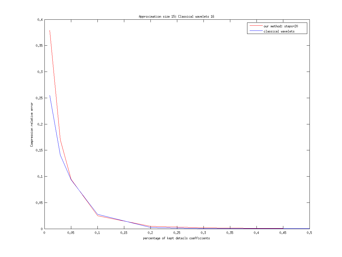
Refer to caption
Figure 8. Relative compression error of signal in Figure 1(a) in terms of the percentage of kept normalized detail coefficients. In red, the error using intertwining wavelets. In blue, error using Daubechies12 wavelets.
Refer to caption
Figure 9. Original signal (blue line) and compressed one (red line) keeping 10% of normalized detail coefficients.

8.3.2. The Minnesota graph.

Figure 10 gives the compressed signal computed with 10% of kept coefficients after 3 multiresolution steps.

Refer to caption
Figure 10. Compression with 10% of kept coefficients. The first graph is the compressed signal, the second one is the error with the original one.

In addition we compare the intertwining wavelets compression results with those obtained through the spectral graph wavelets pyramidal algorithm of [11, 20]. For this purpose, we used the GSPBox11 1 available at https://lts2.epfl.ch/gsp/ [18]. The main features of this pyramidal algorithm are the following ones:

  1. (1)

    Subsampling: 𝒳¯\bar{{\mathcal{X}}} is chosen according to the sign of the highest frequency Fourier mode en−1e_{n-1}.

  2. (2)

    Weighting: ℒ¯\bar{{\mathcal{L}}} is computed by the Schur complement followed by a sparsification step.

  3. (3)

    Approximation coefficients: f¯​(x¯)=g​(t​ℒ)​(x¯)\bar{f}(\bar{x})=g(t{\mathcal{L}})(\bar{x}), where gg is a low-pass filter, and tt is a positive real number. As in [20], we took g⁡(x)=1/(1+x)g(x)=1/(1+x) and t=2t=2 to analyse the signal of Figure 1(b). With this choice, f¯​(x¯)=K1/2​f​(x¯)\bar{f}(\bar{x})=K_{1/2}f(\bar{x}).

  4. (4)

    The signal on 𝒳¯\bar{{\mathcal{X}}} is then interpolated on the whole of 𝒳{\mathcal{X}}: ϵ>0\epsilon>0 being fixed, the interpolation is defined as

    fi​n​t​(x)=(ℒϵ)𝒳​𝒳¯−1​ℒ¯ϵ​f¯​(x),f_{int}(x)=({\mathcal{L}}^{\epsilon})^{-1}_{{\mathcal{X}}\bar{{\mathcal{X}}}}\bar{{\mathcal{L}}}^{\epsilon}\bar{f}(x)\,,

    where ℒϵ=ϵ​Id−ℒ{\mathcal{L}}^{\epsilon}=\epsilon\mbox{Id}-{\mathcal{L}}, and ℒ¯ϵ\bar{{\mathcal{L}}}^{\epsilon} is the Schur complement of ℒ𝒳˘,𝒳˘ϵ{\mathcal{L}}^{\epsilon}_{\breve{{\mathcal{X}}},\breve{{\mathcal{X}}}} in ℒϵ{\mathcal{L}}^{\epsilon}. Using Proposition 1, one can see at once that fi​n​t|𝒳¯=f¯f_{int}|_{\bar{{\mathcal{X}}}}=\bar{f}.

  5. (5)

    The error prediction y=f−fi​n​ty=f-f_{int} is stored.

At the end of one step, the signal f∈ℝ𝒳f\in\mathbb{R}^{{\mathcal{X}}} is encoded by (f¯,y)∈ℝ𝒳¯×𝒳(\bar{f},y)\in\mathbb{R}^{\bar{{\mathcal{X}}}\times{\mathcal{X}}}, resulting in a redundant information. Figure 11 presents the relative compression error in terms of the number of kept coefficients for the two methods. More precisely, we ran the spectral graph wavelets pyramidal algorithm for 7 steps, resulting in 20 approximations coefficients among approximately 2×26422\times 2642 stored ones. We also ran our intertwining wavelets multiresolution until getting approximately the same number of approximation coefficients to get a fair comparison. This took 16 steps, resulting in 16 approximation coefficients. We kept then the same number of the biggest coefficients to construct the compressed version of the signal.

Refer to caption
Figure 11. Relative compression error of signal in Figure 1(b), in terms of the number of kept coefficients. In red, the error using intertwining wavelets. In blue, error using the spectral graph wavelets pyramidal algorithm.

8.3.3. Sensor graph

For the signal on the sensor graph we compare once again in the same way our method with the Pyramid algorithm on 3 steps. In this case we also included the results of our procedure without sparsification, since they surprisingly show that the sparsification improve the results. In Figure 12, we compare the relative compression errors in terms of the number of kept coefficients for the Pyramid algorithm and our method with and without sparsification.

Refer to caption Refer to caption
Without sparsification With sparsification
Figure 12. Relative compression error of signal in Figure 1(c), in terms of the number of kept coefficients. In red, the error using intertwining wavelets. In blue, error using the spectral graph wavelets pyramidal algorithm. In the first graph, we do not sparsify the graph, while we perform sparsification on the second.

Aknowledgements

Marseille’s team thanks Leiden university for its hospitality along many cumulated weeks during which we discovered our wavelets. This was supported by Frank den Hollander’s ERC Advanced Grant 267356-VARIS. The four authors are especially grateful to Dominique Benielli (labex Archimède) who made possible the numerical work. L. Avena was partially supported by NWO Gravitation Grant 024.002.003-NETWORKS.

References

  • [1] Avena, Luca; Castell, Fabienne; Gaudillière, Alexandre; Mélot, Clothilde. Approximate and exact solutions of intertwining equations through random forests. arXiv:1702.05992v1 [math.PR].
  • [2] Avena, Luca; Gaudillière, Alexandre. Two applications of random spanning forests. To appear in Journal of Theoretical Probability. (see arXiv:1310.1723v4 [math.PR] for a preprint version with a different title).
  • [3] Carmona, Philippe; Petit, Frédérique; Yor, Marc. Beta-gamma random variables and intertwining relations between certain Markov processes. Rev. Mat. Iberoamericana 14 (1998), no. 2, 311–367.
  • [4] Coifman, Ronald R.; Maggioni, Mauro. Diffusion wavelets. Applied and Computational Harmonic Analysis, vol. 21, no. 1, pp 53–94, 2006.
  • [5] Cohen, Albert: Numerical analysis of wavelet methods, Studies in mathematics and its applications, Elsevier, Amsterdam, 2003
  • [6] Daubechies, Ingrid: Ten lectures on wavelets. SIAM: Society for Industrial and Applied Mathematics. (1992)
  • [7] Diaconis, Persi; Fill, James Allen. Strong stationary times via a new form of duality. Ann. Probab. 18 (1990), no. 4, 1483–1522.
  • [8] Donati-Martin, Catherine; Doumerc, Yan; Matsumoto, Hiroyuki; Yor, Marc. Some properties of the Wishart processes and a matrix extension of the Hartman-Watson laws. Publ. Res. Inst. Math. Sci. 40 (2004), no. 4, 1385–1412.
  • [9] Elisha, Oren; Dekel, Shai. Wavelet decompositions of random forests. Smoothness analysis, sparse approximation and applications. J. Mach. Learn. Res. 17 (2016), Paper No. 198, 38 pp.
  • [10] Gavish, Matan; Boaz, Nadler; Coifman, Ronald R. Multiscale wavelets on trees, graphs and high dimensional data: theory and applications to semi supervised learning. Proceedings of the 27th International Conference on Machine Learning (2010), 367–374.
  • [11] Hammond, David K.; Vandergheynst, Pierre; Gribonval, Rémi. Wavelets on graphs via spectral graph theory. Applied and Computational Harmonic Analysis (2009), Elsevier 30, no 2, 129–150.
  • [12] Mallat, Stéphane. A wavelet tour of signal processing. Academic Press, (2008)
  • [13] Matsumoto, Hiroyuki; Yor, Marc. An analogue of Pitman’s 2​M−X2M-X theorem for exponential Wiener functionals. I. A time-inversion approach. Nagoya Math. J. 159 (2000), 125–166.
  • [14] Marchal, Philippe. Loop-erased random walks, spanning trees and Hamiltonian cycles. Elect. Comm. Probab. 5 (2000), 39–50.
  • [15] Narang, Sunil K.; Ortega, Antonio. Perfect reconstruction two-channel wavelet filterbanks for graph structured data. IEEE Transactions on Signal Processing 60 (6) (2012), pp 2786–2799.
  • [16] Narang, Sunil K.; Ortega, Antonio. Compact support biorthogonal wavelet filterbanks for arbitrary undirected graphs. IEEE Transactions on Signal Processing 61 (19) (2013), 4673–4685.
  • [17] Nguyen, Ha Q.; Do, Minh N. Downsampling of signal on graphs via maximum spanning tree. IEEE Transactions on Signal Processing 63 (1) (2015), 182–191.
  • [18] Perraudin, Nathanaël; Paratte, Johan; Shuman, David I.; Kalofolias, Vassilis; Vandergheynst, Pierre; Hammond, David K. GSPBOX: A toolbox for signal processing on graphs. ArXiv e-prints, Aug. 2014. http://arxiv.org/abs/1408.5781.
  • [19] Rogers, L. C. G.; Pitman, J. W. Markov functions. Ann. Probab. 9 (1981), no. 4, 573–582.
  • [20] Shuman, David I.; Faraji, Mohamad J.; Vandergheynst, Pierre. A multiscale pyramid transform for graph signals. IEEE Transactions on Signal Processing 64 (8) (2016) , 2119–2134.
  • [21] Shuman, David I.; Narang, Sunil K.; Frossard, Pascal; Ortega, Antonio; Vandergheynst, Pierre. The Emerging Field of Signal Processing on Graphs: Extending High-Dimensional Data Analysis to Networks and Other Irregular Domains. IEEE Signal Processing Magazine 30 (2013), no. 3, 83-98.
  • [22] Tremblay, Nicolas; Borgnat, Pierre. Subgraph-based filterbanks for graph signals. IEEE Transactions on Signal Processing 64 (15) (2016), 3827-3840.
  • [23] Warren, Jon. Dyson’s Brownian motions, intertwining and interlacing. Electron. J. Probab. 12 (2007), no. 19, 573–590.
  • [24] D. Wilson, Generating random spanning trees more quickly than the cover time, Proceedings of the twenty-eighth annual acm symposium on the theory of computing (1996), 296–303.
  • [25] Zhang, Fuzhen (Editor). The Schur complement and its applications. Numerical Methods and Algorithms. Springer (2005).