Finite size analysis of measurement device independent
quantum cryptography with continuous variables

Panagiotis Papanastasiou Affiliation: Computer Science and York Centre for Quantum Technologies, University of York, York YO10 5GH, United Kingdom Carlo Ottaviani Affiliation: Computer Science and York Centre for Quantum Technologies, University of York, York YO10 5GH, United Kingdom Stefano Pirandola Affiliation: Computer Science and York Centre for Quantum Technologies, University of York, York YO10 5GH, United Kingdom

Abstract

We study the impact of finite-size effects on the key rate of continuous-variable (CV) measurement-device-independent (MDI) quantum key distribution (QKD), considering two-mode Gaussian attacks. Inspired by the parameter estimation technique developed in [Ruppert et al. Phys. Rev. A 90, 062310 (2014)] we adapt it to study CV-MDI-QKD and, assuming realistic experimental conditions, we analyze the impact of finite-size effects on the key rate. We find that the performance of the protocol approaches the ideal one increasing the block-size and, most importantly, that blocks between $10^{6}$ and $10^{9}$ data points may provide key rates $\sim 10^{-2}$ bit/use over metropolitan distances.

I Introduction

Quantum key distribution (QKD) [1] promises to allow unconditionally secure (theoretical) communication. Its strength relies on two main elements: The encoding of classical information ( $0$ and $1$ bits) into non-orthogonal quantum states, and the impossibility of perfect discrimination between them. In a conventional QKD protocol two users, Alice and Bob, share quantum systems which are unavoidably corrupted every time that an eavesdropper (Eve) tries to access the information encoded. This perturbation is detectable, and allows the parties to quantify the amount of error-correction and privacy amplification to apply to the shared data, in order to reduce Eve’s information to a negligible amount. Then they can use the obtained key in an one-time pad protocol [2].

The fundamental mechanism of QKD is clearly preserved also in more complex (repeater-based) communication configurations [3, 4], aiming at activating long distance communication and quantum networks. In the basic point-to-point scenario, the recent work [7] succeeded in establishing the secret-key capacity of various quantum channels. The combined use of relative entropy of entanglement [8, 9, 10] and teleportation stretching (which reduces any adaptive protocol to a block-form) enables one to compute the two-way capacity of many important quantum channels (see Ref. [7] and further works [11, 12, 13, 14, 15] for the correct definition and rigorous use of teleportation stretching in quantum communication, quantum metrology and channel discrimination). The result of Ref. [7] sets the fundamental limit of point-to-point QKD and, as such, it marks the edge when private communication inevitably needs quantum repeaters. This benchmark has already had a wide application in recent works [16, 21, 22, 23, 24, 25, 26, 28, 20, 19, 17, 29, 18, 27].

Continuous variable (CV) quantum systems [30], in particular Gaussian systems [31], emerged recently as very promising carriers of quantum information. They have the potential to be used for high-rate quantum communication because, rather than using single-photon quantum states and photon-counting, they employ bright coherent states and homodyne detections, which naturally boost the achievable key-rate. Based on this premise, CV QKD protocols [32] have been proposed using one-way [33, 34, 35] or two-way quantum communications [36]. Some one-way schemes have been experimentally realized [38, 39, 37, 40], over remarkably long-distance [41, 42]. Additional theoretical analysis has been focused on QKD with thermal states [43, 44, 45, 46, 47, 48], with an experiment performed [49]. Recently CV-QKD has been extended to a network configuration [50, 52], implementing the general idea of measurement-device-independent (MDI) QKD [53, 54]. Here two parties, unable to access a secure direct link, can be assisted by an intermediate relay (even untrusted) to establish a secure channel.

Many challenges [55] need to be solved, before private quantum networking can become a mature technology. However, CV QKD protocols and their security analysis have progressed rapidly toward more practical and realistic assumptions. In this respect, the incorporation of finite-size effects is particularly important. In fact, when we assume that the parties exchange only a finite number of signals, one expects the deterioration of the key rate. In addition to this, finite-size analysis is also the first step towards a more general security proof within the composable framework [56, 57, 58]. While the theoretical study of the impact of finite-size effects has been done in several previous works [59, 60, 61], CV-MDI QKD has been so far investigated neglecting this aspect and limiting the analysis to the asymptotic regime [62].

In order to start filling this gap, in this work we focus on evaluating the impact of finite-size effects on the key-rate of CV-MDI protocol. This study is important not only because these effects have not yet evaluated in detail for MDI protocols, but also because this type of analysis represents a necessary steps to refine the security analysis of CV-MDI towards the more complete composable scenario. We perform a detailed study of the impact of finite-size effects for both the symmetric [52] and asymmetric configuration [50, 51]. We extend the parameter estimation methods described in Ref. [61], for conventional one-way protocols, to the relay-based communication. We consider Gaussian two-mode attacks which have been already extensively studied in one-way schemes [63], two-way protocols [64, 65] and the CV-MDI setup [66].

We remark that, in our analysis, we work within the Gaussian assumption. This allows us to develop the statistical estimation theory of the relevant parameters of the channels which are their transmissivities and excess noise. The confidence interval of the estimated parameters are then quantified using their variances and setting a $6.5-$ sigma accuracy, which allows us to grant a very low error probability of $\epsilon_{PE}=10^{-10}$ during the parameter estimation procedure. The confidence intervals are used to select the worst-case scenario, by choosing the lower transmissivity of the links and the higher excess-noise available. The key rate is then numerically computed, using the estimated values of transmissivity and noise, and optimized over free parameters, which are the Gaussian modulation of the signals and the ratio between the number of signals used in the parameter estimation and total number of signals exchanged.

As expected we find that, increasing the block-size of the signals exchanged, one recovers the performance under ideal condition. Most importantly, one has that block-size in the range of $10^{6}\div 10^{9}$ signals can provide a positive key rate of about $10^{-2}$ bit/use, in the presence of high excess noise $\varepsilon=0.01$ , and attenuation compatible with the use of standard optical fibres over metropolitan distances. The structure of this paper is the following. In Section II, we present the details of the CV-MDI-QKD protocol. In Section III, we describe the parameter estimation. In Section IV, we discuss the results obtained and finally Section V is for the conclusions.

II Protocol, eavesdropping and key rate

For the sake of clarity, let us first describe the working mechanism of CV-MDI-QKD from the prepare and measure perspective, where Alice and Bob send coherent states, $|\alpha\rangle$ and $|\beta\rangle$ , to an intermediate relay. The amplitudes $\alpha$ and $\beta$ are Gaussian modulated, i.e., each party sends to the relay an average thermal state with variance $V_{M}\geq 0$ . The duty of the relay is very simple: it mixes the incoming signals on a balanced beam splitter and performs a CV Bell detection, i.e., two conjugate homodyne detections on $q_{-}$ and $p_{+}$ , at the output ports of the balanced beam splitter [67].

Refer to caption — Figure 1: The figure shows the EB representation of CV-MDI QKD. Alice and Bob have TMSV states with modes $(a,A)$ and $(b,B)$ . Local modes $a$ and $b$ are kept by the parties, while $A$ and $B$ are sent to the relay through two links with transmittance $\tau_{A}$ and $\tau_{B}$ . When Alice and Bob heterodyne the local modes, the travelling ones $A$ and $B$ are projected onto coherent states $|\alpha\rangle$ and $|\beta\rangle$ . The relay performs a Bell-measurement and broadcast the outcomes $\gamma$ , creating correlation between the parties: for instance, Bob recovers Alice variable $\beta$ by subtracting his variable $\alpha$ from the relay’s outputs $\gamma$ . The Gaussian attack on the links is simulated by Eve using ancillas $E_{1}$ and $E_{2}$ , and thermal noise $\omega_{A}\geq 1$ and $\omega_{B}\geq 1$ , respectively. These ancillary modes are, in general, two-mode correlated (see text for more details). The ancillary outputs are stored in a quantum memory for a later measurement.

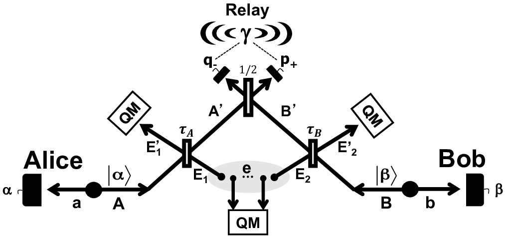
Then, the relay broadcasts the obtained values of $\gamma:=\left(q_{-}+ip_{+}\right)/\sqrt{2}$ . This new variable can also be written as $\gamma:=\alpha-\beta^{\ast}+\hat{\delta}$ , where $\hat{\delta}$ is the detection noise. It is then clear that the relay acts as a correlator for the parties, who can infer each other variable ( $\alpha$ , $\beta$ ) from a simple post-processing [50].

The broadcast of the Bell detection outcomes, $\gamma$ , does not help the eavesdropper who is forced to attack the communication links to the relay, in order to obtain information on amplitudes $\alpha$ and $\beta$ . This operation introduces detectable excess of noise, that the parties can use to quantify Eve’s knowledge on $\alpha$ and $\beta$ (accessible information). From this stage on, the protocol works as any other QKD scheme [1], with the Alice and Bob implementing enough error correction and privacy amplification to reduce Eve’s accessible information to a negligible amount.

II.1 Two-mode eavesdropping

A powerful approach to study the security of any quantum cryptographic protocol is to adopt the entanglement based (EB) representation, where the description of the dynamics takes place in a dilated Hilbert space, which allows to work with pure states. The EB representation of CV-MDI QKD scheme is given in Fig. 1: Alice’s and Bob’s sources of coherent states are purified assuming to start from a two-mode squeezed vacuum (TMSV) states $\rho_{aA}$ and $\rho_{bB}$ , whose zero-mean Gaussian states are completely described by the following identical covariance matrices (CM)

\mathbf{V}_{aA}=\mathbf{V}_{bB}=\begin{pmatrix}\mu\mathbf{I}&\sqrt{\mu^{2}-1}\mathbf{Z}\\ \sqrt{\mu^{2}-1}\mathbf{Z}&\mu\mathbf{I}\end{pmatrix},

(1)

where $\mu=V_{M}+1$ and $\mathbf{Z=}$ diag $(1,-1)$ .

Modes $A$ and $B$ are sent through the links, while local ones, $a$ and $b$ , are heterodyned. The measurements projects the travelling modes into coherent states $|\alpha\rangle$ and $|\beta\rangle$ respectively. The channel attenuation on modes $A$ and $B$ is modeled by two beam splitters with transmissivities $\tau_{A}$ and $\tau_{B}$ , with $0\leq\tau_{A,B}\leq 1$ . These process Alice’s and Bob’s signals with a pair of Eve’s ancillary systems $E_{1}$ and $E_{2}$ which, in general, belong to a wider reservoir of modes controlled by the eavesdropper and including the set $\mathbf{e}$ (which can be neglected in the limit of infinite signals exchanged [68]).

We can then write the dilation of the initial Eve’s state as a two-mode Gaussian state $\sigma_{E_{1}E_{2}}$ described by the following general CM

\mathbf{V}_{E_{1}E_{2}}=\begin{pmatrix}\omega_{A}\mathbf{I}&\mathbf{G}\\ \mathbf{G}&\omega_{B}\mathbf{I}\end{pmatrix},

(2)

where $\mathbf{G=}$ diag( $g,g^{\prime}$ ). The correlation parameters $g$ and $g^{\prime}$ satisfy the constraints given in Ref. [72], while $\omega_{A},\omega_{B}\geq 1$ account for the thermal noise injected by Eve, on each link, during the attack. When $g=g^{\prime}=0$ , the two-mode state $\sigma_{E_{1}E_{2}}$ is a tensor product, which leads to a standard single-mode collective attack realized by two independent entangling cloners [38]. By contrast for $g\neq 0$ and $g^{\prime}\neq 0$ , the two entangling cloners are not independent, and the optimal attack is two-mode coherent, as described in [50, 52, 66].

II.2 Key rate

The EB representation is useful for the security analysis because Alice-Bob reduced output states $\rho_{ab|\gamma}$ and $\rho_{b|\gamma\alpha}$ , described by the CMs $\mathbf{V}_{ab|\gamma}$ and $\mathbf{V}_{b|\gamma\alpha}$ respectively (see Section A for further details), have the same entropies of Eve’s output states. Under the ideal assumption that the parties exchange infinite many signals ( $N\gg 1$ ), and assuming that the parties reconcile over Alice’s data to build the key, one bounds Eve’s accessible information by the Holevo function,

I_{H}:=S(\rho_{ab|\gamma})-S(\rho_{b|\gamma\alpha}),

(3)

where $S(.)$ is the von Neumann entropy. For Gaussian states, we have the simple expression [31]

S=\sum_{x}h(x),

where $x$ is the generic symplectic eigenvalue of the CM, and

	$\displaystyle h(x)$	$\displaystyle=\frac{x+1}{2}\log_{2}\frac{x+1}{2}-\frac{x-1}{2}\log_{2}\frac{x-1}{2},$		(4)
		$\displaystyle\overset{x\rightarrow\infty}{\rightarrow}\log_{2}\frac{e}{2}x.$		(5)

We then can write an expression for the key rate

K^{\infty}:=\xi I_{AB}-I_{H},

(6)

where $\xi\leq 1$ quantifies the inefficiency of error correction and privacy amplification protocols [69, 70, 71] and $I_{AB}$ is Alice-Bob mutual information. This is given by

I_{AB}=\frac{1}{2}\log_{2}\frac{V_{b|\gamma}^{q}+1}{V_{b|\gamma\alpha}^{q}+1}+\frac{1}{2}\log_{2}\frac{V_{b|\gamma}^{p}+1}{V_{b|\gamma\alpha}^{p}+1},

(7)

with $V_{b|\gamma}^{q}$ ( $V_{b|\gamma}^{p}$ ) and $V_{b|\gamma\alpha}^{q}$ ( $V_{b|\gamma\alpha}^{p}$ ) being the variances of CMs $\mathbf{V}_{ab|\gamma}$ and $\mathbf{V}_{b|\gamma\alpha}$ for the position (momentum) quadrature. These CMs are given in Appendix A. The key rate is then function of parameters $\xi$ , $\omega_{A}$ , $\omega_{B}$ , $\tau_{A}$ and $\tau_{B}$ and the Gaussian modulation $V_{M}$ . Its expression can be found in the supplemental information of Ref. [50].

III Channel parameter estimation

In a practical implementation of any QKD protocol, Alice and Bob can only exchange a finite number of signals. In addition, they can only use a portion of these to build the key, being the others used to estimate the channel parameters. In this section we provide a description of CV-MDI QKD, quantifying the impact of finite-size effects and the performance of the protocol. To perform this analysis, we adapt the theory developed in Ref. [61] for one-way CV-QKD. We determine the channel parameters (transmissivity and excess noise) within confidence intervals. Then we choose the worst case scenario, picking the lower transmissivity and higher excess noise within their confidence intervals, so as to minimize the key rate.

III.1 Losses and excess noise at the relay outputs

The outputs variables of the relay are quadratures $q_{-}$ , relative to mode $-$ , and $p_{+}$ for mode $+$ . These depend on the evolution of Alice’s and Bob’s travelling modes $A=(q_{A}$ , $p_{A})$ and $B=(q_{B}$ , $p_{B})$ . In terms of these input field quadratures one can then write the following relations

	$\displaystyle q_{-}$	$\displaystyle=\frac{1}{\sqrt{2}}(\sqrt{\tau_{B}}q_{B}-\sqrt{\tau_{A}}q_{A})+q_{N},$		(8)
	$\displaystyle p_{+}$	$\displaystyle=\frac{1}{\sqrt{2}}(\sqrt{\tau_{B}}p_{B}+\sqrt{\tau_{A}}p_{A})+p_{N},$		(9)

where $q_{N}=q_{\varepsilon}+q_{sn}$ and $p_{N}=q_{\varepsilon}+q_{sn}$ are noise terms accounting for both excess noise and quantum shot noise coming form the signal modes as well as Eve’s ancillary modes. Their variances are given by

V_{q_{N}}=1+V_{q,\epsilon},\text{ \ \ }V_{p_{N}}=1+V_{p,\epsilon},

(10)

with

V_{q,\epsilon}=k-gu,\text{ \ \ }V_{p,\epsilon}=k+g^{\prime}u,

(11)

and

	$\displaystyle k$	$\displaystyle=\frac{(1-\tau_{B})(\omega_{B}-1)+(1-\tau_{A})(\omega_{A}-1)}{2},$		(12)
	$\displaystyle u$	$\displaystyle=\sqrt{(1-\tau_{B})(1-\tau_{A})},$		(13)

where $g$ and $g^{\prime}$ have been defined in Eq. (2).

Now we describe in more detail the parameters estimation procedure. Alice’s and Bob’s Gaussian modulation $V_{M}$ is assumed to be a known parameter. We need to estimate the channel’s transmissivity $\tau_{A}$ , $\tau_{B}$ and variance of the excess noises $V_{q,\epsilon}$ and $V_{p,\epsilon}$ , with their confidence intervals. Assuming that $m$ Gaussian distributed signals are used for this task, we associate to $A_{q,i}$ ( $A_{p,i}$ ) and $B_{q,i}$ ( $B_{p,i}$ ), for $i\in\{1,2,\dots,m\}$ , the empirical realizations of the field quadrature of the traveling modes. By contrast, we denote by $R_{q,i}$ and $R_{p,i}$ the realizations of the relay outputs. Let first discuss the dynamics of the quadrature $q$ . From Eq. (8) one can write the estimator of transmissivity $\tau_{A}$ as follows

\hat{\tau}_{Aq}=\frac{2}{V_{M}^{2}}\hat{C}_{AR_{q}}^{2},

where the covariance $C_{AR_{q}}=\sqrt{\tau_{A}/2}V_{M}$ has maximum likelihood estimator given by

\hat{C}_{AR_{q}}=\frac{1}{m}\sum_{i=1}^{m}A_{q,i}R_{q,i},

and to which one can associate the following variance (see Appendix C for more details)

\text{Var}(\hat{\tau}_{Aq})=\frac{8\tau_{A}}{m}\left(\tau_{A}+\frac{\tau_{B}}{2}\right)\left[1+\frac{V_{q,N}}{\left(\tau_{A}+\frac{\tau_{B}}{2}\right)V_{M}}\right].

(14)

Very similar relations hold for the estimator of $\tau_{A}$ obtained considering the other output of the relay, $p_{+}$ . We can write the estimator of the covariance $C_{AR_{p}}$ , which is given by

\hat{C}_{ARp}=\frac{1}{m}\sum_{i=1}^{m}A_{p,i}R_{p,i},

then using Eq. (9) one can write the estimator of the transmissivity $\tau_{A}$

\hat{\tau}_{Ap}=\frac{2}{V_{M}^{2}}\hat{C}_{AR_{p}}^{2},

having variance

\text{Var}(\hat{\tau}_{Ap})=\frac{8}{m}\tau_{A}\left(\tau_{A}+\frac{\tau_{B}}{2}\right)\left[1+\frac{V_{p,N}}{\left(\tau_{A}+\frac{\tau_{B}}{2}\right)V_{M}}\right].

(15)

We notice that it differs from the formula of Eq. (14) for the expression of $V_{p,N}$ , given in Eq. (10). Now, from Eq. (14) and Eq. (15) we calculate the optimum linear combination of the variances of the two estimators

\text{Var}(\hat{\tau}_{A})=\frac{\text{Var}(\hat{\tau}_{A_{q}})\text{Var}(\hat{\tau}_{Ap})}{\text{Var}(\hat{\tau}_{A_{q}})+\text{Var}(\hat{\tau}_{Ap})}:=\sigma_{A}^{2}.

(16)

The same steps can be performed to obtain the relevant estimators for transmissivity $\tau_{B}$ and the corresponding variance Var $(\hat{\tau}_{B})=\sigma_{B}^{2}$ .

Now we write the estimator of the variance of the excess noise present on the communication links, $V_{q,\epsilon}$ . This can be derived from the maximum likelihood estimator for $V_{q,N}$ , and it reads

\hat{V}_{q,\epsilon}=\frac{1}{m}\sum_{i=1}^{m}\left[R_{q,i}-\frac{1}{\sqrt{2}}(\sqrt{\hat{\tau}_{B}}B_{q,i}-\sqrt{\hat{\tau}_{A}}A_{q,i})\right]^{2}-1,

(17)

with variance (Appendix C)

\text{Var}(\hat{V}_{q,\epsilon})\approx\frac{2}{m}V_{q,N}^{2}:=s_{q}^{2}.

(18)

Correspondingly, we obtain an estimator for $V_{p,\epsilon}$ expressed as

\hat{V}_{p,\epsilon}=\frac{1}{m}\sum_{i=1}\left[R_{p,i}-\frac{1}{\sqrt{2}}(\sqrt{\hat{\tau}_{B}}B_{p,i}+\sqrt{\hat{\tau}_{A}}A_{p,i})\right]^{2}-1

(19)

and variance

\text{Var}(\hat{V}_{p,\epsilon})\approx\frac{2}{m}V_{p,N}^{2}:=s_{p}^{2}.

(20)

Finally, from Eq. (17) and Eq. (20) we compute the confidence intervals and select the pessimistic values given by the following choice of parameters

	$\displaystyle\tau_{A}^{\text{{low}}}=$	$\displaystyle\tau_{A}-6.5\sigma_{A},\text{ \ \ }\tau_{B}^{\text{{low}}}=\tau_{B}-6.5\sigma_{B},$		(21)
	$\displaystyle V_{q,\epsilon}^{\text{{up}}}=$	$\displaystyle V_{q,\epsilon}+6.5s_{q},\text{ \ \ }V_{p,\epsilon}^{\text{{up}}}=V_{p,\epsilon}+6.5s_{p}.$		(22)

III.2 Secret key rate with finite size effects

Once we have obtained the estimation of the transmissivities of the links and the corresponding excess noises, we can write the key rate, incorporating finite size effects writing

K=\frac{n}{\bar{N}}\left(K^{\infty}(\xi,V_{M},\tau_{A}^{\text{{low}}},\tau_{B}^{\text{{low}}},V_{q,\epsilon}^{\text{{up}}},V_{p,\epsilon}^{\text{{up}}})-\Delta(n)\right),

(23)

where $n=\bar{N}-m$ is the number of signals used to prepare the key and $\bar{N}$ the total number of signal exchanged. The key rate is then computed replacing the values of Eq. (21) and Eq. (22) in the asymptotic key rate of Eq. (6). In particular, first one computes the key rate $R$ of Eq. (23), using the Holevo function of Eq. (3) for the channel parameters given by Eq. (21) and (22). Then, in order

to account for the penalty for using the Holevo function even if we have a finite number of signals exchanged, one must include the correction term

\Delta(n)\sim\sqrt{\frac{1}{n}\log_{2}2\varepsilon_{PA}^{-1}}

which depends on the number of signals used to prepare the key, $n$ , and the probability of error related to the privacy amplification procedure $\varepsilon_{PA}$ . A detailed description of this correction term can be found in Ref. [60].

IV Results

The key rate of the asymmetric configuration of the relay is described in the top-panel (a) of Fig. 2. We plot the key rate as a function of Bob’s channel transmissivity, expressed in terms of dB of attenuation, while the transmissivity of Alice’s link is set to $\tau_{A}=0.98$ . The curves are obtained considering two-mode optimal attacks, for which $g=-g^{\prime}$ with $g=\min\left[\sqrt{(\omega_{A}-1)(\omega_{B}+1)},\sqrt{(\omega_{B}-1)(\omega_{A}+1)})\right]$ and $\omega_{A}\sim\omega_{B}\sim 1.01$ [50] and using the key rate of Eq. (23) incorporating also finite-size effects. The efficiency of classical code for error correction and reconciliation efficiency is set to $\xi=0.98$ , and the final key rate is optimized over the variance of the Gaussian modulation $V_{M}$ (see Fig. 3) and the ratio $r=n/\bar{N}$ . The black-solid line gives the asymptotic key rate for very large $\bar{N}$ ( $>>10^{9}$ ), while the dashed line is for block-size $\bar{N}=10^{9}$ and the dot-dashed line is obtained for $\bar{N}=10^{6}$ .

The bottom panel in Fig. 2 (b), plots the secret key rate for the symmetric case [52] ( $\tau_{A}=\tau_{B}$ ). The curves are obtained setting all the other parameters as in Fig. 2 (a) and optimizing as before the key rate for the case including finite-size effects. The black solid line describes again the asymptotic case $\bar{N}\rightarrow\infty$ of the symmetric configuration while the dashed lines is obtained for $\bar{N}=10^{9}$ and the dotted one for $\bar{N}=10^{6}$ .

Let us finally remark on a couple of points. First, we notice that the performance of finite-size CV-MDI-QKD converges to the ideal one if the number of signal exchanged increases. Second, according to the plots, we notice that the key rate of the CV-MDI-QKD protocol is sufficiently robust with respect to the finite size effects, with block sizes of $10^{9}$ points approaching the asymptotic limit.

V Conclusion

In conclusion, we have studied the security of Gaussian CV-MDI-QKD taking into account finite-size effects. These emerge when one assumes that the parties exchange only a finite number of signals during the quantum communication stage. In our analysis we assumed imperfect efficiency of error correction and privacy amplification $(\xi<1)$ and developed the finite-size analysis adapting the channel parameters estimation approach described in Ref. [61]. The resulting finite size key rate has then been optimized over the Gaussian modulation and the number of signals used to perform the parameter estimation.

Our results show that, also considering finite-size effects under realistic conditions, CV-MDI QKD over metropolitan distances is feasible within today state-of-the-art experimental conditions. In particular, we found that the adoption of block-size in the range $\bar{N}=10^{6}\div 10^{9}$ is already sufficient in order to achieve a high key rate of $10^{-2}$ bits/use over metropolitan distances, and in the presence of an excess of noise $\varepsilon=0.01$ (SNU).

Finally we underline that the present analysis does not put a final word on the performances of finite-size CV-MDI-QKD. The validity of the described analysis is in fact restricted to the case of Gaussian attacks. Further studies are needed where finite-size effects are investigated within the composable security framework.

See Ref. [73] for a fully composable security proof of CV-MDI-QKD.

Note added. Shortly after the submission of our manuscript, an independent work [74] has been posted on the arXiv. Also this work studies the impact of finite-size blocks on the key-rate of CV-MDI QKD.

VI Acknowledgements

C.O. acknowledges Cosmo Lupo for useful discussions. This work has been supported by the EPSRC via the ‘UK Quantum Communications HUB’ (Grant no. EP/M013472/1).

Appendix A covariance matrices and symplectic eigenvalues

For the sake of clarity, in this section we re-write the CMs and the relevant symplectic eigenvalues derived in Ref. [50] using the notation adopted in the main text. The CM describing the total output state of Alice and Bob, after the relay measurements, $\rho_{ab|\gamma}$ , is given by the following expression

	$\displaystyle\mathbf{V}_{ab\|\gamma}$	$\displaystyle=\begin{pmatrix}(V_{M}+1)\mathbf{I}&0\\ 0&(V_{M}+1)\mathbf{I}\end{pmatrix}-V_{M}(V_{M}+2)\times$
		$\displaystyle\times\begin{pmatrix}\frac{\tau_{A}}{\varphi}&0&-\frac{\sqrt{\tau_{A}\tau_{B}}}{\varphi}&0\\ 0&\frac{\tau_{A}}{\varphi^{\prime}}&0&\frac{\sqrt{\tau_{A}\tau_{B}}}{\varphi^{\prime}}\\ -\frac{\sqrt{\tau_{A}\tau_{B}}}{\varphi}&0&\frac{\tau_{B}}{\varphi}&0\\ 0&\frac{\sqrt{\tau_{A}\tau_{B}}}{\varphi^{\prime}}&0&\frac{\tau_{B}}{\varphi^{\prime}}\end{pmatrix},$		(24)

where

	$\displaystyle\varphi$	$\displaystyle=(\tau_{A}+\tau_{B})V_{M}+2+2V_{\epsilon,g},$		(25)
	$\displaystyle\varphi^{\prime}$	$\displaystyle=(\tau_{A}+\tau_{B})V_{M}+2+2V_{\epsilon,g^{\prime}}$		(26)

and where we have defined

	$\displaystyle V_{\epsilon,g}=$	$\displaystyle\frac{1}{2}\left(\bar{\tau}_{B}(\omega_{B}-1)+\bar{\tau}_{A}(\omega_{A}-1)-2g\sqrt{\bar{\tau}_{B}\bar{\tau}_{A}}\right),$		(27)
	$\displaystyle V_{\epsilon,g^{\prime}}=$	$\displaystyle\frac{1}{2}\left(\bar{\tau}_{B}(\omega_{B}-1)+\bar{\tau}_{A}(\omega_{A}-1)+2g^{\prime}\sqrt{\bar{\tau}_{B}\bar{\tau}_{A}}\right),$		(28)

with $\bar{\tau}_{l}=1-\tau_{l}$ , for $l=A,B$ .

Bob’s output CM after the double conditioning, first with respect the relay measurements and then after Alice’s heterodyne detection, $\mathbf{V}_{ab|\gamma}$ , is given by

\mathbf{V}_{b|\gamma\alpha}=\begin{pmatrix}\frac{2(V_{M}+1)(1+V_{\epsilon,g})-\tau_{B}V_{M}}{2(1+V_{\epsilon,g})+\tau_{B}V_{M}}&0\\ 0&\frac{2(V_{M}+1)(1+V_{\epsilon,g^{\prime}})-\tau_{B}V_{M}}{2(1+V_{\epsilon,g^{\prime}})+\tau_{B}V_{M}}.\end{pmatrix}

which has the following symplectic eigenvalue given by the $\sqrt{.}$ of the determinant of previous matrix

\bar{\nu}=\sqrt{\det\mathbf{V}_{b|\gamma\alpha}}.

(29)

Appendix B Useful elements of estimation theory

According to the method of maximum likelihood estimation, for a bivariate normal distribution $X=(X_{1},X_{2}$ ), the estimators for the mean $\mu=(\mu_{1},\mu_{2})$ and the covariance matrix $\mathbf{V}$ are given by

	$\displaystyle\hat{\boldsymbol{\mu}}=$	$\displaystyle\frac{1}{m}\sum_{i=1}^{m}\mathbf{X}_{i}$		(30)
	$\displaystyle\widehat{\mathbf{V}}=$	$\displaystyle\frac{1}{m}\sum_{i=1}^{m}(\mathbf{X}_{i}-\hat{\boldsymbol{\mu}})(\mathbf{X}_{i}-\hat{\boldsymbol{\mu}})^{T}$		(31)

where $\mathbf{X}_{i}$ is the $i$ -th statistical realization out of $m$ realizations of $\mathbf{X}$ .

The central limit theorem states that, assuming $m$ realizations $X_{1},X_{2},\dots,X_{m}$ ( $m\gg 1$ ) of a random variable $X$ with unknown density function $f$ , mean $\mu$ and variance $\sigma^{2}<\infty$ , the sample mean

\bar{X}=\dfrac{1}{m}\sum_{i=1}^{m}X_{i}

(32)

is approximately normal with mean $\mu$ and variance $\sigma^{2}/m$ . In order to estimate the mean value of a variable $Y$ , that depends on the square of a variable $X$ for which we have $m$ realizations, we can use the following result: For $m$ realizations $X_{i}$ , for $i=1,2,\dots,m$ , of a normally distributed variable $X$ , having mean $\mu$ and unit variance, the variable

Y=\sum_{i=1}^{m}X_{i}^{2}\sim\chi^{2}\left(k,\lambda\right)

(33)

is distributed according to the $\chi^{2}$ distribution with $k=m$ degrees of freedom and $\lambda=m\mu^{2}$ . The mean value and variance of the chi-squared distribution is given by

\mathbb{E}(Y)=k+\lambda,

(34)

and

\text{Var}(Y)=2(k+2\lambda).

(35)

Let us assume to have two estimators $\hat{s}_{1}$ and $\hat{s}_{2}$ , with variances $\sigma_{1}^{2}$ and $\sigma_{2}^{2}$ , for the same quantity $s$ acquired by different processes. We then compute the optimal linear combination of the variances by the following formula

\sigma_{\text{{opt}}}^{2}=\frac{\sigma_{1}^{2}\sigma_{2}^{2}}{\sigma_{1}^{2}+\sigma_{2}^{2}}.

(36)

Appendix C Variances of the channel parameter estimators

Let us suppose that $A_{q,i}$ ( $B_{q,i}$ ) are independent variables each one following the normal distribution $q_{A}$ ( $q_{B}$ ) with zero mean, variance $V_{M}$ as described in III.1. Accordingly, $R_{q,i}$ ( $R_{p,i}$ ) are assumed to be independent variables following the normal distribution of $q_{R}$ ( $p_{R}$ ), i.e. the relay output variable.

C.1 Variance of the transmissivity

For the covariance between modes $A$ and $R$ , we can write the following estimator

\hat{C}_{AR_{q}}=\frac{1}{m}\sum_{i=1}^{m}A_{q,i}R_{q,i}

(37)

normally distributed as the sample mean of variable $Z=A_{q}R_{q}$ . We can compute the expectation value by

\mathbb{E}(\hat{C}_{AR_{q}})=\mathbb{E}(q_{A}q_{R})=\sqrt{\frac{\tau_{A}}{2}}V_{M}=C_{AR_{q}},

(38)

and the variance can be defined as

V_{\text{{Cov}}}:=\text{{Var}}(\hat{C}_{AR_{q}})

(39)

with

$\displaystyle\text{{Var}}(\hat{C}_{AR_{q}})$	$\displaystyle=\frac{1}{m}\text{{Var}}(q_{A}q_{R})=$
	$\displaystyle=\frac{1}{2m}\left[\tau_{A}\text{{Var}}(q_{A}^{2})+\tau_{B}\text{{Var}}(q_{A}q_{A,B})\right]$
	$\displaystyle+\text{{Var}}(q_{A}q_{N}),$	(40)
	$\displaystyle=\frac{1}{m}\left(\tau_{A}V_{M}^{2}+\frac{\tau_{B}}{2}V_{M}^{2}+V_{M}V_{q,N}\right)$
	$\displaystyle=\frac{1}{m}\left(\tau_{A}+\frac{\tau_{B}}{2}\right)V_{M}^{2}\left[1+\frac{V_{q,N}}{\left(\tau_{A}+\frac{\tau_{B}}{2}\right)V_{M}}\right],$	(41)

where we have considered the independence of the variables and the second order moments of the normal distribution.

Therefore, we can derive the mean and variance for the estimator of $\tau_{A}$ . We rewrite the estimator as

\hat{\tau}_{Aq}=\frac{2V_{\text{{Cov}}}}{V_{M}^{2}}\left(\frac{\hat{C}_{AR_{q}}}{\sqrt{V_{\text{{Cov}}}}}\right)^{2}.

(42)

Note that the variable $\left(\hat{C}_{AR_{q}}/\sqrt{V_{\text{{Cov}}}}\right)^{2}$ is $\chi^{2}-$ distributed, i.e.,

\left(\frac{\hat{C}_{AR_{q}}}{\sqrt{V_{\text{{Cov}}}}}\right)^{2}\sim\chi^{2}\left[1,\left(\frac{C_{AR_{q}}}{\sqrt{V_{\text{{Cov}}}}}\right)^{2}\right],

(43)

with expectation value

\mathbb{E}\left[\left(\frac{\hat{C}_{AR_{q}}}{\sqrt{V_{\text{{Cov}}}}}\right)^{2}\right]=1+\left(\frac{C_{AR_{q}}}{\sqrt{V_{\text{{Cov}}}}}\right)^{2},

(44)

and variance

\text{Var}\left[\left(\frac{\hat{C}_{AR_{q}}}{\sqrt{V_{\text{{Cov}}}}}\right)^{2}\right]=2\left[1+2\left(\frac{C_{AR_{q}}}{\sqrt{V_{\text{{Cov}}}}}\right)^{2}\right].

(45)

The expectation value of $\hat{\tau}_{Aq}$ is then given by

	$\displaystyle\mathbb{E}(\hat{\tau}_{Aq})$	$\displaystyle=\frac{2V_{\text{{Cov}}}}{V_{M}^{2}}\left[1+\left(\frac{C_{AR_{q}}}{\sqrt{V_{\text{{Cov}}}}}\right)^{2}\right]=$
		$\displaystyle=\frac{2C_{AR_{q}}^{2}}{V_{M}^{2}}+\mathcal{O}(1/m)=\tau_{A}+\mathcal{O}(1/m)$		(46)

and its variance is

	$\displaystyle\text{Var}(\hat{\tau}_{Aq})$	$\displaystyle=\frac{4V_{\text{Cov}}^{2}}{V_{M}^{4}}2\left[1+2\left(\frac{C_{AR_{q}}}{\sqrt{V_{\text{Cov}}}}\right)^{2}\right]=$
		$\displaystyle=\frac{16V_{\text{Cov}}C_{AR_{q}}^{2}}{V_{M}^{4}}+\mathcal{O}(1/m^{2}).$		(47)

By replacing from Eq. (38) and Eq. (41), we obtain

$\displaystyle\text{Var}(\hat{\tau}_{Aq})$	$\displaystyle=\frac{16}{mV_{M}^{4}}\left(\tau_{A}+\frac{\tau_{B}}{2}\right)$
	$\displaystyle\frac{V_{M}^{4}\tau_{A}}{2}\left[1+\frac{V_{q,N}}{\left(\tau_{A}+\frac{\tau_{B}}{2}\right)V_{M}}\right]+\mathcal{O}(1/m^{2}),$	(48)
	$\displaystyle=\frac{8\tau_{A}}{m}\left(\tau_{A}+\frac{\tau_{B}}{2}\right)\left[1+\frac{V_{q,N}}{\left(\tau_{A}+\frac{\tau_{B}}{2}\right)V_{M}}\right]$
	$\displaystyle+\mathcal{O}(1/m^{2}).$	(49)

Clearly, as previously noted in [61], the estimator of the transmissivity $\hat{\tau}_{Aq}$ is only asymptotically unbiased. In fact the standard deviation $\sqrt{\text{Var}(\hat{\tau}_{Aq})}$ is of order $1/\sqrt{m}$ while the bias goes as $1/m$ . As we consider $m>10^{5}$ in our analysis, the value of the bias become rapidly negligible as $m\gg 1$ , and the use of estimators $\hat{\tau}_{A}$ and $\hat{\tau}_{B}$ very accurate.

C.2 Variance of the excess noise

Also in our estimation procedure for the MDI protocol, in analogy to the theory developed in Ref. [61], the variance of the estimator can be obtained replacing the estimator of $\tau_{A}$ ( $\tau_{B}$ ) with its value. This simplifies the calculations. Now, we can assume that any uncertainty in the estimator of the excess noise obtained from broadcast results of relay’s measurements on quadrature $q$

\hat{V}_{q,\epsilon}=\frac{1}{m}\sum_{i=1}^{m}\left[R_{q,i}-\frac{\sqrt{\hat{\tau}_{B}}B_{q,i}-\sqrt{\hat{\tau}_{A}}A_{q,i}}{\sqrt{2}}\right]^{2}-1,

(50)

comes only from variables $R_{q,i}$ , $A_{q,i}$ and $B_{q,i}$ . We then have that the expression inside square brackets is normally distributed with zero mean and variance $V_{q,N}$ . In addition to this one also has that the following expression

Y:=\sum_{i=1}^{m}\left(\frac{R_{q,i}-\left(\sqrt{\tau_{B}}B_{q,i}-\sqrt{\tau_{A}}A_{q,i}\right)/\sqrt{2}}{\sqrt{V_{q,N}}}\right)^{2}\sim\chi^{2}(m,0),

(51)

is $\chi^{2}$ -distributed, and has mean $\mathbb{E}(Y)=m$ and variance $\text{Var}(Y)=2m$ . This allows to approximate the sum of Eq. (50) with $V_{q,N}Y$ when we assume large values for $m$ , obtaining the expectation value

\mathbb{E}(\hat{V}_{q,\epsilon})\approx\frac{1}{m}V_{q,N}\mathbb{E}(Y)-1=V_{q,\epsilon}

(52)

and the variance

\text{Var}(\hat{V}_{q,\epsilon})\approx\frac{1}{m^{2}}V_{q,N}^{2}\text{Var}(Y)=\frac{2}{m}V_{q,N}^{2}.

(53)

References

[1] N. Gisin, G. Ribordy, W. Tittel, and H. Zbinden, Rev. Mod. Phys. 74, 145 (2002).
[2] B. Schneier, Applied Cryptography (John Wiley & Sons, New York, 1996).
[3] H. J. Briegel, W. Dür, J. I. Cirac, and P. Zoller, Phys. Rev. Lett. 81, 5932 (1998).
[4] L. M. Duan, M. Lukin, J. I. Cirac, and P. Zoller, Nature 414, 413 (2001).
[5] H. J. Kimble, Nature 453, 1023 (2008).
[6] S. Pirandola and S. L. Braunstein, Nature 532, 169 (2016).
[7] S. Pirandola, R. Laurenza, C. Ottaviani, and L. Banchi, Nat. Commun. 8, 15043 (2017). See also arXiv:1510.08863 and arXiv:1512.04945 (2015).
[8] V. Vedral, M. B. Plenio, M. A. Rippin, and P. L. Knight, Phys. Rev. Lett. 78, 2275 (1997).
[9] V. Vedral and M. B. Plenio, Phys. Rev. A 57, 1619 (1998).
[10] V. Vedral, Rev. Mod. Phys. 74, 197 (2002).
[11] S. Pirandola, Capacities of repeater-assisted quantum communications, arXiv:1601.00966 (2016).
[12] R. Laurenza, and S. Pirandola, General bounds for sender-receiver capacities in multipoint quantum communications, arXiv:1603.07262 (2016). In press on Physical Review A.
[13] T. P. W. Cope, L. Hetzel, L. Banchi, and S. Pirandola, Phys. Rev. A 96, 022323 (2017).
[14] R. Laurenza, S. L. Braunstein, and S. Pirandola, Finite-resource teleportation stretching for continuous-variable systems, arXiv:1706.06065 (2017).
[15] S. Pirandola, and C. Lupo, Phys. Rev. Lett. 118, 100502 (2017).
[16] R. Namiki, L. Jiang, J. Kim, and N. Lütkenhaus, Phys. Rev. A 94, 052304 (2016).
[17] K. Bradler, T. Kalajdzievski, G. Siopsis, and C. Weedbrook, Absolutely covert quantum communication, arXiv:1607.05916 (2016).
[18] B. A. Bash, N. Chandrasekaran, J. H. Shapiro, and S. Guha, Quantum Key Distribution Using Multiple Gaussian Focused Beams, arxiv:1604.08582 (2016).
[19] J. H. Shapiro, Q. Zhuang, Z. Zhang, J. Dove, and F. N. Wong, Floodlight Quantum Key Distribution, in Lasers Congress 2016 (ASSL, LSC, LAC), OSA Technical Digest (online) (Optical Society of America, 2016), paper LTu5B.1.
[20] C. Ottaviani, R. Laurenza, T. P. W. Cope, G. Spedalieri, S. L. Braunstein, and S. Pirandola, Proc. SPIE 9996, 999609 (2016).
[21] M. Pant, H. Krovi, D. Englund, and S. Guha, Phys. Rev. A 95, 012304 (2017).
[22] F. Ewert and P. van Loock, Phys. Rev. A 95, 012327 (2017).
[23] A. Khalique and B. C. Sanders, Opt. Eng. 56, 016114 (2017).
[24] F. Rozpedek, K. Goodenough, J. Ribeiro, N. Kalb, V. Caprara Vivoli, A. Reiserer, R. Hanson, S. Wehner, and D. Elkouss, Realistic parameter regimes for a single sequential quantum repeater, arXiv:1705.00043 (2017).
[25] K. Bradler, and C. Weedbrook, A security proof of continuous-variable QKD using three coherent states, arXiv:1709.01758 (2107).
[26] N. Lo Piparo, N. Sinclair, and M. Razavi, Memory-assisted quantum key distribution resilient against multiple-excitation effects, arXiv:1707.07814 (2017).
[27] N. Lo Piparo, and M. Razavi, Memory-assisted quantum key distribution immune to multiple-excitation effects, Conference on Lasers and Electro-Optics (CLEO), 5-10 June 2016.
[28] N. Lo Piparo, M. Razavi, W. J. Munro, Memory-Assisted Quantum Key Distribution with a Single Nitrogen Vacancy Center, arXiv:1708.06532 (2017).
[29] M. Pant, H. Krovi, D. Towsley, L. Tassiulas, L. Jiang, P. Basu, D. Englund, and S. Guha, Routing entanglement in the quantum internet, arXiv:1708.07142 (2017).
[30] S. L. Braunstein and P. van Loock, Rev. Mod. Phys. 77, 513 (2005).
[31] C. Weedbrook, S. Pirandola, R. García-Patrón, N. J. Cerf, T. C. Ralph, J. H. Shapiro, and S. Lloyd, Rev. Mod. Phys. 84, 621 (2012).
[32] E. Diamanti and A. Leverrier, Entropy 17, 6072 (2015).
[33] F. Grosshans and P. Grangier, Phys. Rev. Lett. 88, 057902 (2002).
[34] C. Weedbrook, A. M. Lance, W. P. Bowen, T. Symul, T. C. Ralph, and P. K. Lam, Phys. Rev. Lett. 93, 170504 (2004).
[35] V. C. Usenko and F. Grosshans, Phys. Rev. A 92, 062337 (2015).
[36] S. Pirandola, S. Mancini, S. Lloyd, and S. L. Braunstein, Nat. Phys. 4, 726 (2008).
[37] T. Gehring, C. S. Jacobsen, and U. L. Andersen, Quantum Information and Computation 16, 1081 (2016).
[38] F. Grosshans, G. Van Ache, J. Wenger, R. Brouri, N. J. Cerf, and P. Grangier, Nature 421, 238 (2003).
[39] J. Lodewyck, M. Bloch, R. García-Patrón, S. Fossier, E. Karpov, E. Diamanti, T. Debuisschert, N. J. Cerf, R. Tualle-Brouri, S. W. McLaughlin et al., Phys. Rev. A 76 (4), 042305 (2007).
[40] L. S. Madsen, V. C. Usenko, M. Lassen, R. Filip, and U. L. Andersen, Nat. Commun. 3, 1083 (2012).
[41] P. Jouguet, S. Kunz-Jacques, A. Leverrier, P. Grangier, and E. Diamanti, Nat. Photon. 7, 378 (2013).
[42] D. Huang, P. Huang, D. Lin, and G. Zeng, Sci. Rep. 6, 19201 (2016).
[43] R. Filip, Phys. Rev. A 77, 022310 (2008).
[44] C. Weedbrook, S. Pirandola, S. Lloyd, and T. C. Ralph, Phys. Rev. Lett 105, 110501 (2010).
[45] V. C. Usenko and R. Filip, Phys. Rev. A 81, 022318 (2010).
[46] C. Weedbrook, S. Pirandola, and T. C. Ralph, Phys. Rev. A 86, 022318 (2012).
[47] C. Weedbrook, C. Ottaviani, and S. Pirandola, Phys. Rev. A 89, 012309 (2014).
[48] V. C. Usenko and R. Filip, Entropy 18, (2016)
[49] C. S. Jacobsen, T. Gehring, and U. L. Andersen, Entropy 17, 4654 (2015).
[50] S. Pirandola, C. Ottaviani, G. Spedalieri, C. Weedbrook, S. L. Braunstein, S. Lloyd, T. Ghering, C.S. Jacobsen, and U. L. Andersen, Nat. Photon. 9, 397 (2015).
[51] G. Spedalieri, C. Ottaviani, S. L. Braunstein, T. Gehring, C. S. Jacobsen, U. L. Andersen, and S. Pirandola, Proc. SPIE 9648, 96480Z (2015).
[52] C. Ottaviani, G. Spedalieri, S. L. Braunstein, and S. Pirandola, Phys. Rev. A 91, 022320 (2015).
[53] S. L. Braunstein and S. Pirandola, Phys. Rev. Lett. 108, 130502 (2012).
[54] H. K. Lo, M. Curty, and B. Qi, Phys. Rev. Lett. 108, 130503 (2012).
[55] V. Scarani, H. Bechmann-Pasquinucci, N. J. Cerf, M. Dusek, N. Lütkenhaus, and M. Peev, Rev. Mod. Phys. 81, 1301 (2008).
[56] F. Furrer, T. Franz, M. Berta, A. Leverrier, V. B. Scholz, M. Tomamichel, and R. F. Werner, Phys. Rev. Lett. 109, 100502 (2012).
[57] A. Leverrier, Phys. Rev. Lett. 114, 070501 (2015).
[58] A. Leverrier, Phys. Rev. Lett. 118, 200501 (2017).
[59] V. Scarani and R. Renner, Phys. Rev. Lett. 100, 200501 (2008).
[60] A. Leverrier, F. Grosshans, and P. Grangier, Phys. Rev. A 81, 062343 (2010).
[61] L. Ruppert, V. C. Usenko, and R. Filip, Phys. Rev. A 90, 062310 (2014).
[62] I. Devetak and A. Winter, Proc. R. Soc. London A 461, 207 (2005).
[63] C. Ottaviani, S. Mancini, and S. Pirandola, Phys. Rev. A 95, 052310 (2017).
[64] C. Ottaviani and S. Pirandola, Sci. Rep. 6, 22225 (2016).
[65] C. Ottaviani, S. Mancini, and S. Pirandola, Phys. Rev. A 92, 062323 (2015).
[66] C. Ottaviani, G. Spedalieri, S. L. Braunstein, and S. Pirandola, arXiv:1509.04144, (2015).
[67] G. Spedalieri, C. Ottaviani, and S. Pirandola, Open Systems & Information Dynamics 20, 1350011 (2013).
[68] S. Pirandola, S. L. Braunstein, and S. Lloyd, Phys. Rev. Lett. 101, 200504 (2008).
[69] P. Jouguet, S. Kunz-Jacques, and A. Leverrier, Phys. Rev. A 84, 062317 (2011).
[70] M. Milicevic, C. Feng, L. M. Zhang, P. G. Gulak, arXiv:1702.07740, (2017).
[71] X. Wang, Y.-C. Zhang, Z. Li, B. Xu, S. Yu, H. Guo, arXiv:1703.04916, (2017).
[72] S. Pirandola, New J. Phys. 15, 113046 (2013).
[73] C. Lupo, C. Ottaviani, P. Papanastasiou, and S. Pirandola, arXiv:1704.07924, (2017).
[74] X. Zhang, Y.-C. Zhang, Y. Zhao, X. Wang, S. Yu, H. Guo, arXiv:1707.05931, (2017).

Finite size analysis of measurement device independent quantum cryptography with continuous variables