IFT-UAM/CSIC-17-048
FTUAM-17-09
Production of vector resonances at the LHC via -scattering:
a unitarized EChL analysis
R. L. Delgado1** * rafael.delgado.lopez@ucm.es, A. Dobado1†† † dobado@fis.ucm.es, D. Espriu2‡‡ ‡ espriu@icc.ub.edu, C. Garcia-Garcia3§§ § claudia.garcia@uam.es, M.J. Herrero3¶¶ ¶ maria.herrero@uam.es, X. Marcano3∥∥ ∥ xabier.marcano@uam.es, J.J. Sanz-Cillero1**** ** jjsanzcillero@ucm.es
1Departamento de Física Teórica I, Universidad Complutense de Madrid,
Plaza de las Ciencias 1, 28040 Madrid, Spain
2Departament de ¬•Física Quàntica i Astrofísica and Institut de Ciències del Cosmos (ICCUB), Universitat de Barcelona, Martí i Franquès 1, 08028 Barcelona, Catalonia, Spain
3Departamento de Física Teórica and Instituto de Física Teórica, IFT-UAM/CSIC,
Universidad Autónoma de Madrid, Cantoblanco, 28049 Madrid, Spain
Abstract
In the present work we study the production of vector resonances at the LHC by means of the vector boson scattering and explore the sensitivities to these resonances for the expected future LHC luminosities. We are assuming that these vector resonances are generated dynamically from the self interactions of the longitudinal gauge bosons, and , and work under the framework of the electroweak chiral Lagrangian to describe in a model independent way the supposedly strong dynamics of these modes. The properties of the vector resonances, mass, width and couplings to the and gauge bosons are derived from the inverse amplitude method approach. We implement all these features into a single model, the IAM-MC, adapted for MonteCarlo, built in a Lagrangian language in terms of the electroweak chiral Lagrangian and a chiral Lagrangian for the vector resonances, which mimics the resonant behavior of the IAM and provides unitary amplitudes. The model has been implemented in MadGraph, allowing us to perform a realistic study of the signal versus background events at the LHC. In particular, we have focused our study on the type of events, discussing first on the potential of the hadronic and semileptonic channels of the final , and next exploring in more detail the clearest signals. These are provided by the leptonic decays of the gauge bosons, leading to a final state with , , having a very distinctive signature, and showing clearly the emergence of the resonances with masses in the range of 1.5-2.5 TeV, which we have explored.
1 Introduction
One of the most likely indications of the existence of physics beyond the standard model (SM) could be the appearance of resonances in the scattering of longitudinally polarized and electroweak (EW) gauge bosons. This would be a formidable hint of the existence of new interactions involving the electroweak symmetry breaking sector (EWSBS) of the SM. This possibility is indeed contemplated in all composite Higgs scenarios, characterized by the existence of a scale GeV where some new strong interactions trigger the dynamical breaking of a global symmetry group to a certain subgroup . The Goldstone bosons that appear provide the longitudinal degrees of freedom of the weak gauge bosons, while the Higgs boson would be one of the leftover Goldstone bosons. A non-zero mass for the latter is often provided by electroweak radiative corrections, e.g., via some misalignment mechanism between the gauge group and the global unbroken subgroup [1].
In the present work we will not assume any specific model for the strong dynamics underlying the EWSBS nor for the above mentioned misalignment mechanism. Instead, we will work under the generic and minimal assumptions for the above global groups and the spontaneous symmetry breaking pattern given by . This involves the minimal set of Goldstone bosons that are needed to generate the EW gauge boson masses, and , and also preserves the wanted custodial symmetry . This symmetry protects the SM tree level relation from potentially dangerous strong dynamics corrections, keeping the values of the masses close to each other. Under these generic assumptions, the most convenient approach to study in a model independent way the phenomenology of the strongly interacting EWSBS is provided by the electroweak chiral Lagrangian that is based on the above EW chiral symmetry breaking pattern and has the same EW gauge symmetries as the SM. The use of these effective chiral Lagrangians in the context of the electroweak theory was initiated long ago in the eighties [2, 3, 4, 5, 6, 7, 8] by following the guiding lines of the well established chiral perturbation theory (ChPT) of low energy QCD [9, 10, 11]. It was used in the early nineties for LEP phenomenology [12, 13], and for LHC prospects [14, 15, 16, 17], and it has received an important push and upgrade in the last years, mainly after the discovery of the Higgs particle. All this lead to the building of the EW chiral Lagrangian with a light Higgs (EChL) [18, 19, 20, 21, 22, 23, 24, 25, 26, 27, 28]. A great effort has also been done in exploring the main implications of the EChL for LHC phenomenology (see, for instance, [29] for a recent summary), although no strongly interacting signal from the EWSBS has been seen yet at the LHC. The absence of these signals at present and past colliders is translated, within the EChL framework, into experimental bounds on the size of the a priori unknown chiral parameters of the EChL [30, 23, 31, 32, 33, 34, 27, 35].
One of the most characteristic features of strong dynamics is undoubtedly the appearance of resonances in the spectrum, thus one should also expect new resonances if the EWSBS is strongly interacting. The use of the EChL for the study of this strong dynamics suggests that the scale associated to these resonances is related to the parameter with dimension of energy controlling the perturbative expansion within this chiral effective field theory, given typically, in the minimal scenario that we work with, by . Therefore, one expects resonances to appear with masses typically of a few TeV, clearly in the range covered at the LHC. The theoretical framework for the description of such resonances is, however, not universal and one has to rely on a particular (author dependent) approach. Once one chooses, as we do, the approach provided by the EChL, there are basically two main paths to proceed. Either the resonances are introduced explicitly at the Lagrangian level and the new terms added to the EChL are required to share the same symmetries of this latter, in particular the EW chiral symmetry, or they are not explicitly included but they are instead dynamically generated from the EChL itself. The first approach has been followed in several works [36, 37, 38, 39, 40] essentially along the lines of previous works within the context of low energy QCD [41]. This type of chiral resonances have also been studied at the LHC [42]. The second approach has been followed in a number of works that use the inverse amplitude method (IAM) to impose the unitarity of the amplitudes predicted with the EChL [20, 24, 21, 22, 43, 25, 28, 44, 45, 46]. Within this approach, the self-interactions of the longitudinal EW bosons, which are assumed to be strong, are the responsible of the dynamical generation of the resonances, and these are expected to show up in the scattering of the longitudinal modes, and , essentially as it happens in the context of ChPT where the QCD resonances emerge in the scattering of pions [47, 48, 49, 50]. The IAM was indeed used long ago in the context of the strongly interacting EWSBS framework but without the Higgs particle, and the production of these IAM resonances at the LHC was also addressed [51, 14, 15]. The advantage of this second approach is that it provides unitary amplitudes, which are absolutely needed for a realistic analysis at the LHC, and it predicts the properties of the resonances, masses, widths and couplings, in terms of the chiral parameters of the EChL. The disadvantage of this method is that it does not deal with full amplitudes but with partial waves, which are not very convenient for a MonteCarlo analysis at the LHC.
The present work addresses the question of whether these IAM dynamically generated resonances of the EWSBS could be visible at the LHC by means of the study of the EW vector boson scattering (VBS). These VBS processes are the most relevant channels to explore at the LHC if the longitudinal gauge modes are really strongly interacting, since they involve the four point self-interactions of the EW gauge bosons. Moreover, the resonances should emerge more clearly in VBS processes as they are generated from this strong dynamics. Our study aims to quantify the visibility of these resonances and also to determine the integrated luminosities that would be required to this end. More concretely, our purpose here is to estimate the event rates at the LHC of the production of a triplet vector resonance, , via scattering, and the subsequent decays of the final and . We have selected this particular subprocess because it has several appealing features in comparison with other VBS channels. In the presence of such dynamical vector resonances, these emerge/resonate (in particular, the charged ones) in the s-channel of , whereas in other subprocesses like , , and do not. Other interesting cases like where the neutral resonance, , could similarly emerge in the s-channel have, however, severe backgrounds. For this reason it is known to be very difficult to disentangle the signal from the SM irreducible background at the LHC. In particular, the SM one-loop gluon initiated subprocess, , turns out to be a very important background in this case due to the huge gluon density in the proton at the LHC energies. Our selected process , in contrast, does not suffer from this background, and therefore it provides one of the cleanest windows to look for these vector resonances at the LHC.
Consequently, our theoretical framework will be: 1) the effective electroweak chiral theory with a light Higgs boson in terms of the ‘chiral’ effective couplings, , and and effective Higgs boson couplings (custodial symmetry of the underlying strong dynamics will be assumed); 2) the unitarization of via the IAM, following the works [21, 22, 44, 43, 20, 24, 25, 28] and making sure that the predictions at the LHC comply with the obvious requirement of unitarity; 3) we work with EW gauge bosons in the external legs of the VBS amplitudes and not with Goldstone bosons. This means that we go beyond the simpler predictions provided by the equivalence theorem (ET) [52, 53, 54, 55], and this will allow us to make realistic predictions for massive and gauge bosons production and their decays at the LHC; 4) out of the EChL we shall construct and effective Lagrangian including vector resonances, based on the Proca 4-vector formalism [36, 37, 38, 39, 40], in order to introduce in a Lagrangian language the resonances that are dynamically generated by the IAM. This effective Lagrangian includes the proper resonance couplings to the and and have the symmetries of the EChL, in particular the EW Chiral symmetry. With this Lagrangian we will mimic the resonant behavior of the IAM amplitudes, having the resonance masses and widths as predicted by the IAM. Indeed, we will make use of this vector Lagrangian to extract the Lorentz structure of the scattering vertex to be coded in the MonteCarlo. The coupling itself will turn out to be a momentum-dependent function that will be derived from the IAM unitarization process in the channel. This IAM-MC model presented here is proper for a MonteCarlo analysis and it is included in MadGraph5 [56] for this work. The corresponding UFO file for the present IAM-MC model can be provided on demand. We would like to emphasize that our IAM-MC model provides full amplitudes with massive external EW gauge bosons. The corresponding cross section is computed from these full amplitudes and not from the first partial waves that do not provide a sufficiently accurate result, as we have checked.
Finally, a careful study of the signal versus backgrounds for the full process , leading to events with two jets plus one and one will be performed. We will first discuss on the potential of the hadronic and semileptonic channels of the final . Then we will explore the cleanest channels leading to events with two jets and the three leptons and missing energy which come from the leptonic decays of the final and . For that study we will employ the well established VBS selection cuts [57, 58, 59, 60] and some specific optimal cuts on the final particles, which will eventually allow us to extract the emergent vector resonances from the SM background in this kind of events at the LHC.
The paper is organized as follows. In section 2 we summarize the main features of the EChL. In section 3 we present the predictions for the scattering process within this EChL framework, we unitarize the corresponding amplitudes with the IAM, and we select specific EChL scenarios with emergent vector resonances in this scattering process. Section 4 is devoted to the presentation of our IAM-MC model and the description of how we deal with IAM vector resonances in scattering within a MonteCarlo framework. In section 5 we present our numerical results for the production and sensitivity to vector resonances in events at LHC. A dicussion on the extrapolated rates for the hadronic and semileptonic channels is also included. The leptonic channels leading to events are also explored in this section. A comparative study of the signal and background events is included. The final section summarizes our main conclusions. The final appendices collect some of our analytical results and Feynman rules for the VBS amplitudes.
2 The Effective Electroweak Chiral Lagrangian
Given that the possible physics existing beyond the minimal SM is model dependent, even after restricting ourselves to the realm of strongly EWSBS, it is necessary to employ a technology that is as model independent as possible. The appropriate tool to do so is provided by the effective EChL. In this theory the information about the underlying microscopic theory is encoded in a number of so-called low-energy constants, i.e., coefficients of local operators.
The EChL is a gauged non-linear effective field theory (EFT) coupled to a singlet scalar particle that contains as dynamical fields the EW gauge bosons, , and , the corresponding would-be Goldstone-bosons, , , and the Higgs scalar boson, . We will not discuss the fermion sector in this article. The , are described by a matrix field that takes values in the coset, and transforms as under the action of the global group . We will assume here that the scalar sector of the EChL preserves the custodial symmetry, except for the explicit breaking due to the gauging of the symmetry. We believe that this assumption is well justified, since experimental measurements involving the well known parameter, or the effective couplings that parametrize the interaction between the Higgs and the EW gauge bosons show no evidence of custodial breaking in the bosonic sector other than that induced from .
The basic building blocks of the gauge invariant EChL are the following:
| (1) | |||||
| (2) | |||||
| (3) | |||||
| (4) | |||||
| (5) | |||||
| (6) |
According to the usual counting rules, the invariant terms in the EChL are organized by means of their ‘chiral dimension’, meaning that a term with ‘chiral dimension’ will contribute to in the corresponding power momentum expansion. The chiral dimension of each term in the EChL can be found out by following the scaling with of the various contributing basic functions. Derivatives and masses are considered as soft scales of the EFT and of the same order in the chiral counting, i.e. of . The gauge boson masses, and are examples of these soft masses in the case of the EChL. These are generated from the covariant derivative in Eq. (3) once the field is expanded in terms of the fields as:
| (7) |
where the dots represent terms with higher powers of and whose precise form will depend on the particular parametrization of . Once the gauge fields are rotated to the physical basis they get the usual gauge boson squared mass values at lowest order: and .
In order to have a power counting consistent with the loop expansion one needs all the terms in the covariant derivative above to be of the same order. Thus, the proper assignment is , and or, equivalently, , , . In addition, we will also consider in this work the Higgs boson mass as another soft mass in the EChL with a similar chiral counting as and . That implies, , or equivalently , with being the SM Higgs self-coupling.
With these building blocks one then constructs the EChL up to a given order in the chiral expansion. We require this Lagrangian to be invariant, Lorentz invariant, gauge invariant and custodial preserving. For the present work we include the terms with chiral dimension up to , therefore, the EChL can be generically written as:
| (8) |
where refers to the terms with chiral dimension 2, i.e , refers to the terms with chiral dimension 4, i.e , and and are the gauge-fixing (GF) and the corresponding non-abelian Fadeev-Popov (FP) terms. The relevant terms for the description of EW gauge boson scattering amplitudes are11 1 Our notation is taken from [61, 62] and compares: 1) with [3] as, , , , , ; 2) with [11] as, , , , ; and with [10] as, , , , .:
| (9) | ||||
| (10) |
Regarding the present experimental constraints on the previous EW chiral coefficients, we have summarized in Fig. 1 the most recent available set from the literature [30, 23, 31, 32, 33, 34, 27, 29, 35].
From the previous set of constraints we can see that the most constrained EW chiral couplings at present are , from its relation with the oblique parameter, and where the most important constraints come from its relation with the anomalous triple gauge couplings. Also is constrained, although more mildly, by triple gauge couplings. On the other hand, the chiral couplings and are constrained mainly by the studies of the anomalous quartic gauge couplings at the LHC and LEP [23, 32, 34, 35]. In addition, is constrained to be close to the SM value () up to deviations, the coefficient is unknown so far, see however [43]. Regarding and , the best constraint comes from the related coefficient appearing in the photonic Lagrangian term. It has been experimentally constrained to [27]. A recent summary of constraints and some phenomenological issues of for LHC physics can be found in [29].
3 Selection of scenarios with vector resonances in scattering
In this section we present the specific EChL scenarios that will be explored in our forthcomming study at the LHC, having dynamical vector resonances emerging in scattering. First we show the results of the cross-sections for from the EChL, which are compared with the SM predictions. Then we unitarize these EChL results, and finally, within these unitarized results, we select the scenarios with emergent vector resonances .
Even though all the EW chiral coefficients in the previously introduced EChL will enter in the description of the subprocesses of our interest, i.e. the scattering of EW gauge bosons, not all of them are equally relevant for all channels. As stated in the introduction, here we will be mostly interested in studying the deviations with respect to the SM predictions for the specific scattering process , since it provides one of the cleanest windows to look for charged vector resonances at the LHC. On the other hand, we know by means of the ET [52, 53, 54, 55], which applies to renormalizable gauges and is valid also for the EChL [63, 64, 65, 66], that the scattering amplitude for this subprocess can be approximated, at large energies compared to the gauge boson masses, by the scattering amplitude of the corresponding would-be Goldstone bosons,
| (11) |
Since the relevant EW chiral coefficients in the amplitude (i.e., those that remain even switching off the gauge interactions, ), are just , , and , we conclude that for our purpose of describing the most relevant departures from the SM in it will be sufficient to work with just this subset of EChL parameters.
As we have said, in the present work we deal with massive gauge bosons in the external legs of the VBS amplitudes and not with their corresponding Goldstone bosons. The various contributing terms from the EChL to the EW gauge boson scattering amplitude of our interest are the following:
| (12) |
where the leading order (LO), , and next to leading order contributions (NLO), , are denoted as and respectively, and are given by:
| (13) |
For completeness, we have also collected in the appendices the necessary Feynman rules, Feynman diagrams and resulting scattering amplitudes, for the simplest case of a tree level computation, i.e.,
| (14) |
The analytical result is given in terms of the three EChL parameters, , and involved, and has been found with the help of FeynArts [67] and FormCalc [68]. We have also included in the appendices the corresponding results for the SM amplitude at the tree level, to illustrate clearly the differences with respect to the EChL results. It should be noticed that the parameter does not enter in scattering at the tree level, and it just enters in . It should also be noticed that, to our knowledge, a full one-loop EChL computation is not available in the literature for this process, i.e., the full analytical result of is unknown. However, we will use an approximation to estimate the size of this one-loop contribution, following [20, 24, 25]. Concretely, the real part of the loop diagrams is computed using the ET (but keeping ) and the imaginary part of the loops is calculated exactly through the tree-level result by making use of the optical theorem. In the following, we will refer to this NLO computation, , as quasi exact one-loop EChL result.
We have chosen one example to illustrate numerically and graphically the energy behavior of the EChL cross section and the comparison with the SM prediction. This is displayed in Fig. 2, where the chiral parameters have been set to , , and . As we can see in Fig. 2 the predictions from the EChL grow with energy, and they depart clearly from the SM prediction which for is nearly flat with energy in the explored interval of GeV. This growth is more pronounced as larger the values of and/or are, and it leads to amplitudes that cross over the unitarity bound at some energy , whose particular value obviously depends on the assumed parameters. We have checked that by using input parameters in the allowed region by the experimental constraints in Fig. 1, this crossing, which is defined in terms of the partial waves as , may indeed occur at the TeV energies explored by the LHC, even for as small values as . For instance, in the example of Fig. 2 this crossing takes place first for the partial wave, and it happens at around 2 TeV. Larger values of would lead to the unitarity violation happening at even lower energies.
At this stage, it is also interesting to comment on the goodness of our assumption of neglecting other loop contributions in our computation of scattering. In particular, as we have said, we are ignoring in this work the contributions from fermions. Since the fermions would only contribute via loops to this scattering process, and since the dominant contributions would come from the third generation-quark loops, we have performed an estimate of the size of these loop contributions to be sure that they are indeed negligible. For this estimate we have assumed that all the fermion interactions are the same as in the SM and we have used the analytical results of [69] which are provided for the SM within the ET. Our numerical estimate of the heavy fermion loops indicates that for the high energies of our interest here, say between 1 and 3 TeV, the contributions from the top loops to decrease with , in contrast to the contributions from the EChL loops which increase with energy, and they are indeed very small, between pb and pb. These are more than three orders of magnitude below the prediction of from the EChL (specifically, from our quasi exact prediction in Fig. 2). Therefore we conclude that our assumption in this work of ignoring the fermion loops is well justified.
The above commented deviations of the EChL predictions with respect to the SM ones in the scattering of longitudinally polarized gauge bosons, are by themselves an interesting result and suggest that they could lead to signals above the SM background given by an enhancement in events with in the final state. However, the polarization of the final gauge bosons is not expected to be measured at the LHC, and therefore the realistic SM background will come from the full unpolarized SM cross section. The relevance of the various polarization channels in the SM prediction is shown in Fig. 3. We display the different polarization cross sections integrated in two choices of the center of mass scattering angle, and . We have checked that we get the same results with FormCalc and MadGraph5. It is clear that the channel (gray lines in Fig. 3) is the dominant one, then go and (pink lines) which we denote together here and along this work as , and next (orange lines). For instance, in the energy interval GeV, the size of is approximately one order of magnitude smaller than that of the . Therefore, in order to extract clear signals at the LHC from departures in the channel we will have to produce cross-sections emerging above this irreducible SM background. It is one of our main motivations here to consider dynamically generated resonances as leading emergent signals from the EChL in scattering, instead of considering just smooth enhancements over the SM background.
Finally, the previously mentioned violation of unitarity of the EChL scattering amplitudes leads to our major concern in this work: the need of an unitarization method in order to provide realistic predictions at the LHC. We choose here one of the most used unitarization methods for the partial waves, the IAM, which has the advantage over other methods of being able to generate dynamically the vector resonances that we are interested in. In terms of fixed isospin and angular momentum , and following a similar notation as in Eq. (12), for the LO and NLO contributions, the IAM partial waves are given by (for a review, see for instance Ref. [70]):
| (15) |
Other unitarization procedures such as N/D and the improved K matrix (IK) were also studied and compared with the IAM in the present context in detail in Ref. [71]. In this reference the IAM, N/D and the IK unitarization methods are implemented in a particular way compatible with the electroweak chiral expansion. All of these three methods turn out to be acceptable, since they produce partial waves which are: IR and UV finite, renormalization scale independent, elastically unitary, have the proper analytical structure (they feature a right and a left cut) and they reproduce the expected low energy results of the EChL up to the one-loop level. Thus the three methods can provide an UV completion of the low-energy chiral amplitudes. Moreover, for some region of the chiral couplings parameter space, they can have a pole in the second Riemann sheet with similar properties. These poles have a natural interpretation as dynamically generated resonances with the quantum numbers of the corresponding channel22 2 The simplest and better known case, where this machinery is known to work very well, is provided by scattering. There, unitarization of the partial wave provides the position and properties of the meson when the measured values of the low-energy chiral couplings in the chiral Lagrangian are used. Note that these couplings are measured at energies well below . Likewise determining the corresponding anomalous coefficients in VBS at the LHC would give valuable information on resonances to be found at higher values of .. By comparison of the three methods for different values of the chiral couplings it is possible to realize that all of them normally produce the same qualitative results and, in many cases, the agreement is also quantitative up to high energies. This is particularly true for the channel. However, as it is explained in detail in Ref. [71], the N/D and the IK methods cannot be applied to the channel considered in this work in the particular case of , since it leads to contributions from the left and right cuts which cannot be separated in a -invariant way, as required by these two methods. Therefore, in the following we will use only the IAM method. Contrary to the perturbative expansion of the EChL amplitudes, the IAM amplitudes fulfill all the analyticity and elastic unitarity requirements. In addition, may or may not exhibit a pole as discussed above. If present, it can be interpreted as a dynamically generated resonance. In that case we use here the usual convention for the position of the pole in terms of the mass, , and width, , of the corresponding resonance : . Finally, it is worth mentioning that the IAM is actually derived from the re-summation of bubbles in the s-channel and therefore accounts for re-scattering effects. The dynamical generation of resonances can be understood from the inclusion of this infinite chain of diagrams. Concretely, in the present case of scattering, such re-summation of infinite bubbles in the s-channel means in practice to consider the sequential chain of diagrams with and in the internal bubbles, i.e., . The charged vector resonance is then understood as emerging from this chain.
The solution to the position of the pole in the case of is very simple if the ET is used, and gives simple predictions for the mass and the width of the dinamically generated vector resonances in terms of the EChL parameters, , , and , given by [21, 22]:
| (16) | ||||
| (17) |
with and the scale dependent parameters whose running equations for arbitrary and can be found in [20, 24, 25, 21, 22]. These solutions apply to narrow resonances, i.e., for , which is indeed our case. It should be noticed that, as it is well known, the case with cannot be treated in the IAM within the ET framework. This will not be the case in our quasi-exact predictions, as we will see in the following.
The solution to the position of the pole in the quasi-exact case with is more involved [20, 24, 25], but it basically shares the main qualitative features of the previous ET results. First, the main contribution from the parameters and appears also in the particular combination which is -scale independent if . We have checked explicitly that other contributions from and not going as vanish in the isospin limit where . Second, the main dependence with also comes in the combination , and the main dependence with also comes in the combination . All these generic features can also be seen in our numerical results, displayed in Fig. 4, which we have generated with the FORTRAN code that implements the quasi-exact EChL+IAM framework, borrowed from the authors in Refs. [20, 24, 25].

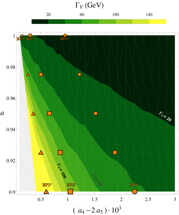
The plots in Fig. 4 show the contour lines of fixed and in the EChL parameter space plane. Here we have explored values of these parameters in the intervals that are allowed by present constraints, specifically, and . The particular contour lines with GeV are highlighted since they will be chosen as our reference mass values in our next study at the LHC. This figure assumes , but we have checked explicitly that other choices for the parameter with do not change appreciably these results. In fact, the contour lines of and in the plane with fixed in the interval (not included here), do not show any appreciable dependence with if this parameter is varied in the interval . The distortions due to are clearly subleading in comparison to the leading effects from and , as explicitly shown in the ET formulas of Eq. (17), and will be neglected from now on. The main reason of this secondary role of , versus , and is because, as we have previously said, in the amplitude enters only via loops, whereas , and enter already at the tree level. Therefore our selection of scenarios will be done in terms of , and , and will be fixed to , for simplicity. This choice of is also motivated in several theoretical models [72, 73, 74]. Our final results will not change appreciably for other choices of .
| BP | ||||||
|---|---|---|---|---|---|---|
| BP1 | ||||||
| BP2 | ||||||
| BP3 | ||||||
| BP1’ | ||||||
| BP2’ | ||||||
| BP3’ |
In Table 1 we present a number of selected benchmark points (BP); namely, some specific sets of values for the relevant parameters and that yield to dynamically generated vector resonances emerging in the channel with masses around the values 1.5, 2 and 2.5 TeV and not to resonances in the (isoscalar) and (isotensor) channels, which we do not consider in this work. These particular mass values for the vector resonances, belonging to the interval (1000, 3000) GeV have been chosen on purpose as illustrative examples of the a priori expected reachable masses at the LHC. In the following sections we will use these benchmark points to predict the visibility of vector resonances that may exist in the channel, and therefore resonate in the process at the LHC. For the channel there are recent alternative studies of the IAM scalar resonances and their production at the LHC, see for instance [46].
The selected points in Table 1 are also included in our previous contour plots in Fig. 4. They are placed at the upper and lower horizontal axes in these plots, and are chosen on purpose at the two boundary values of the parameter: 1) for BP1, BP2 and BP3 and 2) for BP1’, BP2’ and BP3’. These will be our main reference scenarios to which we will devote most of our LHC analysis. However, in order to provide a complementary study of the sensitivity to the parameter we have also defined a family of additional scenarios belonging to these contour lines of fixed , and GeV, respectively, but with different values of in the interval . These BP points are specified by circles, squares and triangles in Fig. 4 and will also be discussed in the final section.
4 Dealing with IAM vector resonances in scattering
In order to study how the vector resonances that are predicted in the IAM could be seen at the LHC with a MonteCarlo analysis, we need first to establish a diagrammatic procedure for scattering to implement the basic ingredients of these IAM resonances in a Lagrangian framework. The use of MonteCarlo event generators like MadGraph requires the model ingredients to be implemented in a Lagrangian language, which means in our case that we have to specify the interactions of the emergent vector resonances with the gauge bosons (and Goldstone bosons). Thus, instead of implementing the scattering amplitude in terms of the predicted IAM partial waves, we simulate this scattering amplitude with a simple model that contains the basic ingredients of the emergent vector resonances. Namely, the mass, the width and the proper couplings to the gauge bosons and . The simplest Lagrangian to include these vector resonances, , that shares the chiral and gauge symmetries of the EChL is provided in Refs. [41, 75, 39, 40]. In the Proca 4-vector formalism, the corresponding -even Lagrangian is given by:
| (18) |
which includes the isotriplet vector resonances, and , via the fields and the a priori free parameters: mass , and couplings and . The basic definitions in Eq. (18) are [37, 38, 36]:
| (21) | ||||
| (22) | ||||
| (23) | ||||
| (24) | ||||
| (25) |
In the unitary gauge (convenient for tree-level collider analyses) we have , and one finds a simpler result. In particular, after rotating to the mass eigenstate basis, where the unphysical mixing terms between the ’s and the gauge bosons (introduced by ) are removed, and after bringing the kinetic and mass terms into the canonical form, we find:
| (26) |
where we have used the short-hand notation (for ), (for ), and .
It should be noticed that in the previous Lagrangian of Eq. (26) there are not interaction terms between the vector resonances and two neutral gauge bosons, , (as there are not either interactions in Eq. (18) of with two neutral Goldstones ) and this explains why the vector resonances cannot emerge in the s-channel of nor 33 3 Notice that scalar resonances could resonate in these channels, but we do not considered them here.. This is a clear consequence of exact custodial invariance and it also confirms that are the proper channels to look for emergent signals from the charged vector resonances . The relevant set of Feynman rules extracted from the above Lagrangian in Eq. (26) is collected in the appendices, for completeness.
Since we are mostly interested here in the deviations with respect to the SM predictions in the case of the longitudinal modes, we will mainly focus on their scattering amplitudes. Therefore, from now on we will simplify our study by setting . This is well justified since this predominantly affects the couplings of the resonances to transverse gauge bosons and, in consequence, is the most relevant coupling to the longitudinal modes. Some additional comments on the behavior of the scattering amplitudes for the other modes will be made at the end of this section.
Our aim here is to use the Lagrangian in Eq. (26) as a practical tool to mimic the main features of the vector resonances found with the IAM. Specifically, we wish to introduce all these features by means of a tree level computation of with . This leads us to the issue of relating , and to the properties of the IAM vector resonances found from . On one hand, the mass and the width are obviously related to the position of the pole, , of . On the other hand, the coupling should also be related to the properties of in the resonant region. For instance, one could extract a value of by identifying the residues of and at . If for simplicity we had used the ET version of the relevant amplitudes, this would have led to the simple relation . Alternatively, one could follow the approach of Refs. [39, 40] where close to the resonance mass shell, they find to be equivalent to a more general Lagrangian44 4 The Lagrangian in Refs. [39, 40] considers the antisymmetric tensor representation for the spin–1 resonances, which is fully equivalent to the Proca four-vector representation provided appropriate non-resonant operators are added to the Lagrangian. in which the on-shell vector coupling is related to the low-energy chiral parameters in the form .
However, this Lagrangian leads to problems if a constant is assumed. Even though it gives a reasonable estimate of the partial wave at , it does not work satisfactorily away from the resonance region. Indeed, it yields to a bad high energy behavior for : the subsequent partial wave grows too fast with energy and crosses the unitary bound at energies of a few TeV. This unwanted violation of unitarity happens, indeed, for any choice of the constant in the Lagrangian . We depict this failure in Fig. 5 for one particular example with , and that produces a IAM vector pole at GeV and GeV, and where we have assumed a constant value of . In this case we have found that the crossing over the unitarity bound occurs at around 3 TeV. From this study, we conclude then that the resulting from with constant does not simulate correctly the behaviour of , which is by construction unitary and therefore we will not take as a constant coupling.
We will define in the following the specific model that we choose to mimic with a chiral Lagrangian the IAM amplitude, which is referred in Fig. 5 as IAM-MC. This will obviously lead us to consider again but with a momentum dependent . This will be done in the next subsection.
4.1 Our model: IAM-MC
We work with the Lagrangian , first introduced in the EW interaction basis in Eqs. (9) and (18), to mimic the IAM amplitude of scattering but with an energy dependent coupling (remember that we are setting in all our numerical estimates), which leads to unitary results in the way that will be described in this subsection. Firstly, our amplitudes have by construction the resonant behavior of the IAM amplitudes at , as commented above. Secondly, it is illustrative to notice that the effective coupling is in fact related to a form factor, as can be seen for instance using a current algebra language. Concretely, the matrix element of a vector current between two longitudinal bosons and the vacuum is described by an energy dependent form factor given by [28]:
| (27) |

where is the interpolating vector current with isospin index that creates a resonance . This form factor can be easily related to at by . In practice, is determined by the matching procedure described next.
In order to build our resonant amplitudes we use the following prescription. First, we impose the matching at the partial waves level. Concretely, it is performed by identifying the tree level predictions from with the predictions from the IAM at , i.e:
| (28) |
where is the partial wave amplitude computed from .
Solving (numerically) this Eq. (28) for the given values of and the corresponding values of leads to the wanted solution for . For instance, in the previous example of , and (our benchmark point BP1’ in Table 1) with corresponding GeV and GeV, we found . For the other selected benchmark points the corresponding values found for are collected in Table 1 and in Fig. 6. Interestingly, these numerical results in Fig. 6 for show a clear correlation with the previously predicted and values in Fig. 4, which fulfill approximately: , as naively expected from the Proca Lagrangian for .
One may notice at this point that the computation of the IAM partial waves has been done with electroweak gauge bosons in the external legs and not with Goldstone bosons. The ET has only been used to compute the real part of the loops involved, as explained before in the previous section.
Away from the resonance we consider an energy dependence in with the following requirements:
- i)
Below the resonance, at low energies, one should find compatibility with the result from , which implies that the predictions from should match those from at these energies. This is what happens indeed to below the resonance, by construction.
- ii)
Above the resonance, at large energies, we require the cross section not to grow faster than the Froissart bound [76], which can be written as:
(29) with and being energy independent quantities. Notice that when using this bound we are implicitly assuming that there are no other resonances (in addition to ) emerging in the spectrum, at least until very high energies.
We have found that these requirements above are well approximated by setting the following simple function:
| (30) |
This coupling should be used when is propagating in the -channel. In the other channels where the resonance could also propagate, and/or channels, the coupling should be the same described in Eq. (30) in terms of the corresponding or variables to be fully crossing symmetric. Nevertheless, we have checked that a completely crossing symmetric energy-dependent coupling, given by , leads to a moderate violation of the Froissart bound in Eq. (29) at energies in the TeV range. To avoid this violation of unitarity, we propose the following expression for the coupling in terms of the and variables:
| (31) |
with corresponding to the channels, respectively, in which the resonance is propagating.
The accuracy of the result with this choice of energy dependent coupling in comparison with the previous constant coupling can be seen in Fig. 5. It is clear from this figure that the result for using this energy dependent coupling simulates much better the IAM result than that with a constant , and it also provides a good low and high energy behaviors. It is worth commenting that we have tried other choices for the dependence with energy of this coupling, but none of these alternative tries have passed all the above required conditions. We have also checked explicitly that our hypothesis in Eqs. (30)-(31) leads to a high-energy behavior of the cross section that is always below and close to the saturation of this Froissart bound.
The above described method, which will be called from now on IAM-MC (named after IAM for MonteCarlo), is the one we choose to simulate the IAM with a Lagrangian formalism. We find that it is the most appropriate one for the forthcoming MonteCarlo analysis with MadGraph5 of LHC generated events.
In summary, we follow the subsequent steps to get for each of the given input values:
- 1)
Compute the amplitude from the tree level diagrams with the Feynman rules from . This gives a result in terms of and .
- 2)
For the given values of , then set and to the corresponding values found from the poles of .
- 3)
Extract the value of by solving numerically Eq. (28).
- 4)
- 5)
Above the resonance we assume that the deviations with respect to the SM come dominantly from , which means in practice that the proper Lagrangian for the computation of the IAM simulated amplitude is rather than . This is obviously equivalent to use with at energies above the resonance.
The detailed description and the analytical results of this computation are collected in the appendices. We emphasize again that these analytical results of the scattering amplitudes do not make use of the ET and they are obtained by a tree level diagrammatic computation with massive external and gauge bosons. For completeness and comparison we have also included in the appendices the predictions for the three cases of our interest, the IAM-MC, the SM, and the EChL, as well as the corresponding Feynman rules.
As for the numerical results, we present in Fig. 7 our predictions of the partial waves for all the selected benchmark points of Table 1. We have also included in these plots the corresponding predictions from the IAM and from the EChL, at both LO and NLO, for comparison. In these plots we clearly see the accuracy of our IAM-MC model in simulating the behavior of the IAM amplitudes. This happens not only at the close region surrounding the resonance, where it is clearly very good, but also below and above the resonance, inside the displayed energy interval of GeV.
For the numerical computation that is relevant for the forthcoming study of the LHC events we will not use the decomposition in partial waves, but the complete amplitude instead. This is an important point, since a description of in terms of only the lowest partial waves would not give a realistic result for energies away from the resonant region, which we have checked explicitly. Therefore, before starting the analysis of the LHC events, it is convenient to learn first about the predictions of the cross section at the subprocess level. Thus, we present in Fig. 8 our numerical results for within our IAM-MC framework and for the same benchmark points of Table 1. In these plots we have also included the predictions from the SM and from the EChL for comparison. What we learn from these figures is immediate: the vector resonances do emerge clearly in the scattering of the longitudinal modes, well above the SM background. We also see that the predictions from the IAM-MC match those from the EChL at low energies, as expected. The main features of the resonances, i.e., the mass, the width and the coupling are obviously manifested in each profile of the resonant IAM-MC lines. It is also worth mentioning our explicit test that all these cross sections in Fig. 8 respect the Froissart unitary bound in Eq. (29).
So far we have been discussing about the predictions of the scattering amplitudes for the longitudinal gauge boson modes. However, for a realistic study with applications to LHC physics, as we will do in the next section, we must explore also the behavior of the scattering of the transverse modes. In fact, the transverse and gauge bosons are dominantly radiated from the initial quarks at the LHC, as compared to the longitudinal ones and, consequently, they will be relevant and have to be taken into account in the full computation. Of course we will make our predictions at the LHC taking into account all the polarization channels as it must be.
To compute the various amplitudes with all the polarization possibilities for being either or , we proceed as described above for the case of the longitudinal modes. We use the same analytical results for the amplitudes given in the appendices in terms of the generic polarization vectors and substitute there the proper polarization vectors according to the corresponding or cases. The numerical results of the cross sections for the most relevant polarizations channels are presented in Fig. 9 for the two benchmark points BP1 and BP1’ that we have chosen as illustrative examples. We have also included the corresponding predictions of the cross sections in the SM for comparison. All these results have been computed with FeynArts and FormCalc, and have been checked with MadGraph5.
Regarding this Fig. 9, one can confirm that at the subprocess level, , the scattering of longitudinal modes in our IAM-MC model clearly dominates over the other polarization channels in the region surrounding the resonance. This is in contrast with the SM case, where the channel dominates by far in the whole energy region studied . This feature of the IAM-MC was indeed expected since, as already said, the coupling affects mainly to the longitudinal modes. Secondly, the predictions of the resonant peaks in the IAM-MC are clearly above the SM background in all the polarization channels that resonate. Thirdly, we also learn that the channel is not the only one that resonates. In fact, also the , and channels manifest a resonant behavior (barely appreciated in the figure in the case) in the IAM-MC, although with much lower cross sections at the peak than the dominant channel. In these examples the hierarchy found in the IAM-MC predictions at the peak is the following:
| (32) |
where is short-hand notation for , and where corresponds to . Also from Fig. 9 one can see that is approximately two orders of magnitude smaller than . Therefore, we conclude that the main features found previously for the , in the region close to the resonance, should emerge in the total cross section, , given the fact that this channel is by far the domminant one. This will be confirmed in the next section. We would like to mention that all the plots presented in this section have been done with FormCalc and checked with MadGraph5.
5 Production and sensitivity to vector resonances in events at the LHC
The process that we wish to explore here is at the LHC via the VBS subprocess , as generically depicted in Fig. 10. Concretely, we select the process with instead of since the former is more copiously produced from the initial protons. However, these type of events containing two gauge bosons and and two jets in the final state can happen at the LHC in many different ways, not only by means of VBS. Therefore, in order to be able to select efficiently these VBS mediated processes, one has to perform the proper optimal cuts in the kinematical variables of the outgoing particles of the collision. These cuts should favor the VBS configuration versus other competing processes. Thus, we are going first to specify our selection of these VBS cuts in terms of the kinematical variables of the two final jets and the final and gauge bosons.
There are many studies in the literature searching for these optimal VBS cuts (see, for instance, Refs. [57, 58, 59, 34, 60]) and where different kinematical variables like transverse momenta, pseudorapidities, and invariant masses of the final particles have been considered. The common feature explored by all these studies is the generic topology showed in these type of VBS mediated events, which have two opposite-sided large pseudorapidity jets together with two gauge bosons, and in our case, within the acceptance of the LHC detectors. This is in contrast to pure QCD events which produce mainly jets in the low pseudorapidity region.
For the present work, we have first selected the cuts in the pseudorapidities of the final jets, , and of the final gauge bosons by giving the following basic VBS cuts: of Ref. [58]. For all the results and plots presented in this section we use MadGraph5, and set the LHC energy to 14 TeV. For the parton distribution functions we set the option NNPDF2.3 [77]. The results from our IAM-MC model, which has been described in the previous section, are generated by means of a specific UFO file that contains the model and the needed four point function of the blob represented in Fig. 10, whose analytical result is also collected in the appendices in terms of the IAM-MC model parameters, see Eqs. (59)-(62). This four point function has obviously momentum dependence and is treated by MadGraph5 as an effective four point vertex which is then used by the MonteCarlo to generate the signal events that we are interested in. With the simplifications assumed in this work, the IAM-MC parameters contained in the UFO file are basically the chiral coefficient and the vector resonance parameters , and , which are fixed from the given input values of , and accordingly to our previous discussion. Concretely, we use the selected points in Fig. 4 to make our predictions with MadGraph5 of the signal events at the LHC from the IAM-MC model.
5.1 Study of the most relevant backgrounds
Regarding the background events from the SM we also generate them with MadGraph5. We only consider here the main irreducible backgrounds since we are assuming that the final and gauge bosons can be reasonably identified and disentangled from pure QCD () events leading to fake ‘’ configurations. For the same reason, we do not consider either the potential backgrounds from top quarks production and decays. This will be totally justified in the final part of this study where we will focus on the leptonic decays of the final and leading to a very clear signal with three leptons, two jets and missing energy in the final state and with very distinct kinematics. We therefore focus here on the two main irreducible SM backgrounds:
- 1)
The pure SM-EW background, from parton level amplitudes of order .
- 2)
The mixed SM-QCDEW background, from parton level amplitudes of order .
We show our predictions of the IAM-MC signal for the selected BP1’ scenario together with those of the two main irreducible SM-EW and SM-QCDEW backgrounds in Fig. 11, for the simple VBS cuts specified in the figure. The selected distributions for this signal versus background comparison are the final jet pseudorapidity, (with being the most energetic jet), and the invariant mass of the two final jets, .
As we can clearly see in this figure, the signal is mainly produced in the interval and with a rather large jet invariant mass of GeV, whereas the SM-QCDEW background is mainly centrally produced, with and at lower invariant masses GeV. Therefore, this suggests our more refined selection of cuts for discriminating the IAM-MC signal from the SM-QCDEW background given by the following optimal VBS cuts:
| (33) |
Regarding the SM-EW background, as we can see in Fig. 11, it has very similar kinematics with respect to our IAM-MC signal in these two jet variables and . This was expected, since, after applying the basic VBS cuts, both receive dominant contributions from the VBS kind of configurations. In order to disentangle our signal from this SM-EW background one has to rely on additional discriminants. As suggested by our previous analysis in section 4, the most powerful of these discriminants would be a devoted study of the final gauge boson polarizations, since the IAM-MC signal produces mainly events whereas the SM-EW background produces mainly events. This latter case can be clearly seen in our results in Fig. 12, where we show the separated predictions of the SM-EW backgrounds for the various polarizations of the final gauge bosons, , + and . Both distributions, the one in the invariant mass of the pair, , and the one in the transverse momentum of the most energetic final jet, , show the clear dominance of the type of events in this SM-EW background. This was expected, since as shown in Fig. 3, the polarizations are practically preserved in the SM, and these background events are basically mediated by , which is the dominant VBS SM channel. We also see in Fig. 12 that the distribution of these SM-EW background events peaks towards lower values in in the events than in the events. This can be understood by the fact that longitudinally polarized vector bosons tend to be emitted at a smaller angle with respect to the beam, and hence smaller transverse momentum, with respect to the incoming quark direction than the transversely polarized ones. As a consequence, the final quark (and thus the final jet) accompanying a longitudinal gauge boson is more forward than the one accompanying a transverse or . This translates into different distributions. Whereas the ones coming from events with transverse gauge bosons tend to peak closer to the EW boson mass, the ones with longitudinally polarized or peak normally around half of the EW boson mass.
These features are very interesting regarding future prospects of polarization studies. As we have argued, being able to disentangle the polarization of the gauge bosons in the final state will be enormously helpful to discriminate signal versus background in these scenarios. Indeed, a more detailed study of the relevant kinematical variables to perform this kind of discrimination deserves some future development, although there are already some analysis in this direction, see for instance Ref. [34]. However, as sophisticated techniques to distinguish among the polarizations of the final and are not yet well stablished, we are not going to use a polarization analysis as a discriminant in this work. We prefer to leave this issue for a forthcoming work. Thus, we will rely in the following in the most obvious and simple way to discriminate the IAM-MC signal and the SM backgrounds, which is by looking for resonant peaks in the invariant mass distributions of the unpolarized cross sections.
5.2 Results for the resonant signal events
In this subsection we present the main results of our IAM-MC resonant signal events together and compared with the relevant backgrounds explored previously. Our predictions of the above mentioned distributions for the IAM-MC signal and of the two main SM backgrounds, SM-QCDEW and SM-EW, are displayed in Fig. 13. We have summarized in these plots the results for all the selected benchmark points in Table 1, after applying the optimal cuts in Eq. (33). We see in these figures that the resonant peaks, coming mainly from the interaction of longitudinally polarized gauge bosons, clearly emerge above the SM backgrounds (dominated by the transverse modes) in all these distributions and in all the studied BP scenarios. In order to quantify the statistical significance of these emergent peaks, we define in terms of the predicted events in our IAM-MC model, , and the background events, , as follows:
| (34) |
with,
| (35) |
Here the event rates are summed over the interval in surrounding the corresponding resonance mass. In the SM predictions we have summed the purely EW contribution and the QCDEW contributions. We display in Table 2 the results for these of the events, for different LHC luminosities: , and , that are expected for the forthcoming runs [78]. We have included the results of two intervals for comparison. First, the events are summed in over the corresponding narrow interval. Second, they are summed over the wider interval around the resonances of . The results differ a bit in the two chosen intervals, as expected, but the conclusions are basically the same: we find very high statistical significances for all the studied BP scenarios in this case of events.
| BP1 | BP2 | BP3 | BP1’ | BP2’ | BP3’ | ||
| 89 (147) | 19 (25) | 4 (9) | 226 (412) | 71 (151) | 33 (59) | ||
| 6 (17) | 2 (4) | 0.3 (2) | 11 (45) | 5 (27) | 3 (14) | ||
| 34.8 (31.1) | 10.8 (9.7) | 6 (5.4) | 64.9 (54.4) | 28.9 (23.8) | 16.1 (12) | ||
| 298 (488) | 64 (82) | 13 (30) | 752 (1374) | 237 (504) | 110 (196) | ||
| 19 (57) | 8 (15) | 1 (6) | 36 (151) | 17 (90) | 11 (46) | ||
| 63.5 (56.8) | 19.8 (17.7) | 11 (9.9) | 118.5 (99.4) | 52.7 (43.5) | 29.3 (22) | ||
| 893 (1465) | 193 (246) | 39 (89) | 2255 (4122) | 710 (1511) | 331 (589) | ||
| 58 (172) | 24 (44) | 3 (17) | 109 (454) | 52 (271) | 34 (139) | ||
| 110 (98.5) | 34.3 (30.6) | 19 (17.1) | 205.3 (172.2) | 91.3 (75.3) | 50.8 (38.1) |
The above predictions in Table 2 are for the selected reference scenarios with the values of the parameter fixed to the borders of the considered interval . In order to study further the sensitivity at the LHC to different values of the parameter within this interval, we have also performed the computation of predicted events, for the additional benchmark points specified in Fig. 4. The results for these new BP’s are collected in Fig. 14. It shows both the predicted event rates, , and statistical significances, , as a function of the parameter, taken within the interval , for an integrated luminosity of . The corresponding rates and significances for the other two luminosities considered here can be easily scaled from these results of . The marked points correspond to our selected BP’s of Fig. 4. As in Table 2, the two lines displayed for each value correspond, respectively, to summing events in the bins contained in the interval of and around each resonance mass. From this Fig. 14 it is clear that the high luminosity LHC with would be sensitive to all values of in through the study of vector resonances with masses of , and TeV. Actually, for this final state, these same conclusions apply to the other two luminosities considered, and .
The previous results for the statistical significances of events are really encouraging. The high statistical significances found show that the resonances would be visible if the and gauge bosons could be detected as final state particles. However, this is not the real case at colliders, and one has to reconstruct ’s and ’s from their decay products. In particular, the study of the so called ‘fat jets’ in the final state, coming from the hadronic decays of boosted gauge bosons, could lead to a reasonably good reconstruction of the and the . The typical signatures of these hadronic events would then consist of four hadronic jets, two thin ones triggering the VBS, and two fat ones triggering the final . If these type of signal events were able to be extracted from the QCD backgrounds, the predicted resonances that we show in Fig. 13 could be very easily discovered. For a fast estimation of the number of signal events and significances that will be obtained by analyzing these kind of hadronic channels with ‘fat jets’ we have performed a naive extrapolation from our results for events by assuming two hypothetical efficiencies for the reconstruction from ‘fat jets’, which we take from the literature [79, 80, 81, 82], and are usually referred to as ‘medium’ with , and ‘tight’ with . The corresponding signal event rates can be extracted simply by [82]:
| (36) |
We show in Fig. 15 our predictions for these naively extrapolated number of events and statistical significances. These results are very encouraging and clearly indicate that with a more devoted study of the and hadronic decays leading to ‘fat jets’ the vector resonances of our selected scenarios would all be visible at the high luminosity option of the LHC with . Looking at the scaled results for other luminosities, one can see that some of the resonances could be seen already for . Concretely, we find that resonances of TeV could be observed at the LHC with this luminosity with statistical significances larger than 11 (6) for all values of the parameter if a medium (tight) reconstruction efficiency is assumed. A medium reconstruction efficiency would also allow to find heavier resonances of 2 (2.5) TeV for values of 0.975 (0.925). The case of , is also very interesting. For this luminosity, the resonances with =1.5 TeV and =2 TeV could all be seen for any value of the parameter between 0.9 and 1 and for the two efficiencies considered. The heaviest ones, with masses of 2.5 TeV, would have significances larger than 3, and therefore could be used to probe values of in the whole interval studied in this work, if a medium efficiency is assumed. For a tight efficiency, one could still be sensitive to values of the parameter between 0.9 and 0.95.
On the other hand, the alternative semileptonic channels where one final EW gauge boson goes to leptons and the other one to hadrons observed as one fat jet, will also lead to interesting signatures like and and are also very promising, with comparable statistics to the previous hadronic channels, as our corresponding naively extrapolated rates (not shown) indicate. The potential of these semileptonic channels can also be inferred from the studies in [35], where they have been used to notably improve the experimental constraints on and by roughly one order of magnitude, with respect to their previous constraints based on the pure leptonic decays [32]. Nevertheless, our previous estimates of event rates involving ‘fat jets’ although really encouraging are yet too naive and deserve further studies for a more precise conclusion. A more realistic and precise computation is needed, but it would require a fully simulated MC analysis of the events with ‘fat jets’ and a good control of the QCD backgrounds and other reducible backgrounds, which is far beyond the scope of this work.
Therefore, from now on, we will focus on the cleanest decays of the and , which are the pure leptonic ones, leading to a final state from the pair with three leptons and one neutrino. Concretely, to unsure a good efficiency in the detection of the final particles we consider just the two first leptonic generations. Therefore, all together, we propose to explore at the LHC events of the type , with being either a muon or an electron, the missing transverse momentum coming from the neutrino, and the two emergent jets from the final quarks that are key to tag the VBS configuration. The event rates in these leptonic channels suffer from a suppression factor of , but have the advantage of allowing us to reconstruct the invariant mass of the pair in the transverse plane, and also to provide a good reconstruction of the .
For the present study of the leptonic channels we apply the set of cuts that are partially extracted from Ref. [59] and optimized as described in the previous background subsection, to make the selection of VBS processes more efficient when having leptons in the final state. These contain all the previous VBS cuts and others, and are summarized by:
| (37) |
where are the pseudorapidities of the jets, is the invariant mass of the jet pair, the invariant mass of the lepton pair coming from the Z decay (this means at least one of the two combinations in the case of with the same lepton flavor), the transverse missing momentum, the transverse momentum of the final leptons, and the transverse invariant mass of the pair defined as follows in terms of the final lepton variables:
| (38) |
with and being the invariant mass and the transverse momentum of the three final leptons respectively, and the transverse momentum of the neutrino.
As before, we generate all the signal, IAM-MC, and background, SM-QCDEW and SM-EW, events with MadGraph5. The results obtained, after applying the previous cuts in Eq. (37), are displayed in Fig. 16, where the total cross section per bin has been plotted as a function of the transverse invariant mass of the pair as defined in Eq. (38) . From this figure we can conclude that the peaks, although smoother, are again clearly seen over the SM backgrounds, specially for the lighter resonances. The shape of the emergent peaks is different than in Fig. 13, typically smaller and broader, as corresponding to distributions with the transverse invariant mass, having the maximum at bit lower values, and getting spread in a wider invariant mass range.
Finally, in order to quantify the statistical significance of these emergent peaks, we have computed the quantity , defined in terms of the predicted number of events from the IAM-MC, , and the background events, , as follows:
| (39) |
with,
| (40) |
The final numerical results for are collected in Table 3. Again, we have considered three different LHC luminosities: , and . The numbers of events presented are the results after summing over the intervals in which we have found the largest statistical significance with at least one IAM-MC event for . In particular we consider the following ranges of :
| (41) |
| BP1 | BP2 | BP3 | BP1’ | BP2’ | BP3’ | ||
| 2 | 0.5 | 0.1 | 5 | 2 | 0.7 | ||
| 1 | 0.4 | 0.1 | 2 | 0.6 | 0.3 | ||
| 0.9 | - | - | 2.8 | 1.4 | - | ||
| 7 | 2 | 0.4 | 18 | 5 | 2 | ||
| 4 | 1 | 0.3 | 6 | 2 | 1 | ||
| 1.6 | 0.3 | - | 5.1 | 2.5 | 1.4 | ||
| 22 | 5 | 1 | 53 | 16 | 7 | ||
| 12 | 4 | 1 | 17 | 6 | 3 | ||
| 2.7 | 0.6 | 0.3 | 8.9 | 4.4 | 2.4 |
As we can see in this Table 3, these more realistic statistical significances for the leptonic channels, are considerably smaller than the previous . However, we still get scenarios with sizable larger than 3. Concretely, the scenarios with leading to vector resonance masses at and below 2 TeV, could be seen in these leptonic channels at the LHC in its forthcoming high luminosity stages. Particularly, for BP1’ with TeV we get sizeable significances around 3, 5, and 9 for luminosities of 300, 1000 and 3000 respectively, whereas for BP2’ with TeV the significances are lower, close to 3 for 1000 and slightly above 4 for 3000 . The scenarios with have comparatively smaller significances, and only the lightest resonances with TeV , like BP1, lead to a significance of around 3 for the highest studied luminosity of 3000 . Notice that there are some cases that we do not consider in our discussion because of the lack of statistics. The scenarios with heavier resonance masses, at and above 2.5 TeV seem to be very difficult to observe, due to the poor statistics for these masses in the leptonic channels. Only our benchmark point BP3’ gets a significance larger that 2 for 3000 . Therefore, in order to get more sizable significances in those cases one would have to perform a more devoted study in other channels like the semileptonic and hadronic ones of the final pair, as we have already commented above.
Finally, we have also explored the additional BP points with different values of the parameter and studied the sensitivities to this parameter in the leptonic channels. The results of the predicted event rates, , and statistical significances, , in terms of the parameter , within the interval are displayed in Fig. 17. From this figure we can clearly conclude that, for the highest luminosity , and for TeV, there will be good sensitivity to the parameter, with larger than 3, in the full interval , except for the limiting value of where is slightly below 3. For the heavier resonances, we find lower sensitivities, with larger than 3 only for TeV and below around 0.94. The case TeV is not very promising to learn about the parameter in the fully leptonic channel except, perhaps, for the scenario with the lowest considered value of where, as said above for BP3’, gets larger than 2. Nevertheless, this would be strongly improved by exploring other decay channels, as we mentioned before.
6 Conclusions
In this work we have explored the production and sensitivity to vector resonances at the LHC. We have worked under the framework of the EChL supplemented by another effective chiral Lagrangian to describe the vector resonances that have the same properties as the dynamically generated resonances found by the IAM. This approach provides unitary amplitudes and effectively takes into account the re-summation of the infinite re-scattering bubbles of the longitudinal gauge bosons which are the dominant ones in the case of a strongly EWSB scenario. We have then built our IAM-MC model that uses this Lagrangian framework and mimics the resonant behavior of the IAM amplitudes. We believe that this IAM-MC framework, where the VBS amplitudes are built from Feynman rules, is the proper one for a MonteCarlo analysis like the one we have done in the present work with MadGraph5. For that purpose we have built the needed UFO file with our IAM-MC model which is ready for other users, upon request. Our IAM-MC model for the vector resonance production at LHC provides unitary VBS amplitudes (we have checked indeed, that the LHC cross sections respect the Froissart bound given by Eq. (29)), and therefore does not require unphysical ad hoc cuts to respect unitarity in the study of the signal versus background events. We also wish to emphasize that our predictions presented here for both the amplitudes and the cross sections are for massive and gauge bosons and are complete in the sense that they are not obtained from the lowest partial waves but from a complete tree level diagrammatic computation.
Concretely, we have focused on the channel which is the most relevant one if one is interested in the study of charged vector resonances from a strongly interacting EWSB. This particular channel is also appealing because it suffers from less sever backgrounds than other channels with two EW vector bosons and two jets in the final state like, for instance, and . With the selection of the proper optimal VBS cuts, the process, , proceeds mainly via the scattering subprocess and it is in this VBS where the resonances of our interest manifest.
We have selected specific benchmark points in the IAM-MC model parameter space which have vector resonances emerging at mass and width values that are of phenomenological interest for the searches at the LHC. Concretely, the fifteen scenarios that we have chosen, summarised in Fig. 4, have their respective resonance masses placed at 1.5 , 2 and 2.5 TeV, and they correspond in our approach to specific values of the relevant EChL parameters, , and in the experimentally allowed region. Specifically, we have considered the intervals and , and set our first six reference scenarios in the borders of the interval: BP1, BP2, and BP3 with and BP1’, BP2’, BP3’ with . These scenarios are used to perform the full study of the MC generated events. The remaining nine scenarios have been used to further explore the sensitivity to the parameter by trying other values in the allowed interval.
We have fully analyzed the event distributions of both the signal and main SM background events with respect to the invariant mass by using MadGraph5, and we have seen clearly the emergence of the vector resonances in all these distributions on top of the SM backgrounds with extremely high statistical significances. Our numerical results are summarised in Fig. 13, Table 2 and in Fig. 14. We have found, indeed, great sensitivity in all the studied scenarios, with masses at 1.5, 2 an 2.5 TeV, and with values of the parameter in the allowed interval . The largest significances are obtained for the lightest resonances with 1.5 TeV and the lowest studied values of , corresponding to our BP1’ scenario, which lead to as large as 65, 118 and 205 for respective luminosities of , and . The lowest significances are obtained for the heaviest resonances with 2.5 TeV and the highest studied value of , corresponding to our BP3 scenario, but they are yet quite sizable, 6, 11 and 19, again for , and , respectively.
These encouraging results for events are assuming that the and the can be fully detected. However, this is not the real case at colliders and one has to rely instead on the partial reconstruction of the final and from their decay products. Thus, in order to profit from the largest rates, we have first discussed the case of the hadronic channels where each EW gauge boson decays into hadrons measured as ‘fat jets’, leading to total signatures of type with four jets, two thin ones triggering the VBS, and two fat ones triggering the final . We have performed a fast estimate of the event rates and significances of these hadronic channels by a naive extrapolation from our results of events. This is done by using the corresponding decay ratios to hadrons and by assuming two hypothetical efficiencies for the reconstruction from ‘fat jets’, ’Medium’ with , and ’Tight’ with following [79, 80, 81, 82]. Our results in Fig. 15 show the big potential of these hadronic channels in the future discovery of these vector resonances, leading to extrapolated significances larger than 3 for all the studied scenarios with masses 1.5, 2 an 2.5 TeV, and values of the parameter in the allowed interval , if the highest luminosity option for the LHC with is assumed. Looking into other luminosities, one can see that some of the resonances could be seen already for . Concretely, we find that resonances of TeV could be observed at the LHC with this later luminosity with statistical significances larger than 11 (6) for all values of the parameter if a medium (tight) reconstruction efficiency is assumed. At this luminosity, a medium reconstruction efficiency would also allow to find heavier resonances of 2 (2.5) TeV for values of 0.975 (0.925). For , the resonances with =1.5 TeV and =2 TeV could all be seen for any value of the parameter between 0.9 and 1 and for the two efficiencies considered. The heaviest ones, with masses of 2.5 TeV, would have significances larger than 3, and therefore could be used to probe values of in the whole interval considered, if a medium efficiency is assumed. For a tight efficiency, one could still be sensitive to values of the parameter between 0.9 and 0.95. We have also commented on the comparable statistics that we get for the extrapolated rates in the case of semileptonic channels of the final leading to signatures like and , showing also the big potential of these channels.
Nevertheless, our previous estimates of event rates involving ‘fat jets’ although really encouraging are not sufficiently precise and we have emphasized that a more realistic and precise computation is needed. This would require a fully simulated MC analysis of the events with ‘fat jets’ and a good control of the QCD backgrounds and other reducible backgrounds, which is far beyond the scope of this work. Instead, we have preferred to study here in full detail the cleanest channels where the final and decay into leptons and to provide our most realistic predictions in those leptonic channels, with lowest rates but with cleanest signatures.
We have then fully studied the golden leptonic and decay channels, i.e., the channels leading to a final state with , , and we have presented the results of the appearing resonances in terms of an experimentally measurable variable, the transverse invariant mass of the final leptons. As it is clearly illustrated in Fig. 16, the shape of the peaks is softened as expected with respect to the final and case, but they are still visible. Our numerical evaluation of the future event rates and sensitivities are summarized in Table 3 and in Fig. 17.
The results in Table 3 demonstrate that with a luminosity of a first hint (with around 3) of resonances with mass around 1.5 TeV for the case could be seen in the leptonic channels. For the first stage of the high luminosity LHC, with , we estimate that these scenarios could be tested with a high statistical significance larger than 5 and a discovery of these resonances with masses close to 1.5 TeV, like in BP1’, could be done. Interestingly, for the last luminosity considered, , all the studied scenarios with resonance masses at and below 2 TeV and with could be seen. Concretely, for BP1’ and BP2’ we get close to 9 and 4 respectively. For the heaviest studied resonances, with masses around 2.5 TeV, small hints with slightly larger than 2 might as well show up in the highest luminosity stage. The sensitivities to other values of in the interval have also been explored. Our numerical results in Fig. 17 show that for the highest luminosity , and for TeV, there will be good sensitivity to the parameter in the leptonic channels, with larger than 3, in the full interval except for the limiting value of where is slightly below 3. For the heavier resonances, we find lower sensitivities, with larger than 3 only for TeV and below around 0.94. The case TeV does not show appreciable sensitivity to , except for the lowest considered value of where, gets larger than 2. Therefore, a fully efficient study of charged vector resonances with masses at (and heavier than) 2.5 TeV would imply to analyze the hadronic and semileptonic channels of the final gauge bosons, as we have already indicated above.
Acknowledgments
We thank P. Arnan for providing us with the FORTRAN code to localize the IAM resonances and for his help at the early stages of this work. A.D. thanks F.J. Llanes-Estrada for previous collaboration. This work is supported by the European Union through the ITN ELUSIVES H2020-MSCA-ITN-2015//674896 and the RISE INVISIBLESPLUS H2020-MSCA-RISE-2015//690575, by the Spanish MINECO through the projects FPA2013-46570-C2-1-P, FPA2014-53375-C2-1-P, FPA2016-75654-C2-1-P, FPA2016-76005-C2-1-P, FPA2016-78645-P (MINECO/ FEDER, EU), by the Spanish Consolider-Ingenio 2010 Programme CPAN (CSD2007-00042) and by the Spanish MINECO’s “Centro de Excelencia Severo Ochoa” Programme under grants SEV-2012-0249 and SEV-2016-0597 and the “María de Maeztu” Programme under grant MDM-2014-0369. X.M. is supported through the Spanish MINECO “Ramón y Cajal” Programme (RYC-2015-17173). R.L.D is supported by the Spanish MINECO grant MINECO:BES-2012-056054, the MINECO project FIS2013-41716-P and the “Ramón Areces” Foundation. We also acknowledge 8000 hours of computer time granted at a small departamental cluster at the UCM.
Appendices
Appendix A Relevant Feynman rules for
In this appendix we collect the relevant Feynman rules, Fig. 18, for the computation of the scattering amplitude in the SM at the tree level. Notice that our conventions here for the SM Feynman rules are the same as in FeynRules [83], except for the sign in the vertex that is opposite. However, this will not give any difference in the predicted amplitudes nor in the predicted events with MadGraph5 (which uses the FeynRules conventions), since this particular vertex always appears squared in all quantities predicted in the present work. We use here and in the following the short notation . We also label the momenta according to the charge of the associated particle. This way, refers to an incoming or a respectively.
Appendix B Relevant Feynman rules for
In this appendix we summarize the relevant EChL Feynman rules, Fig. 19, for the computation of the scattering amplitude at the tree level. These rules come from , defined in Eq. (9), and , defined in Eq. (10), as we are computing up to order . We signal with a gray circle the vertices that receive contributions from the chiral parameters that we consider in this work, and . We also present these Feynman rules with the SM common part singled out for an easier comparison.
Appendix C Relevant Feynman rules for
In this appendix we summarize the relevant Feynman rules, Fig. 20, for the computation of the scattering amplitude in our IAM-MC at the tree level. These rules come from , defined in Eq. (9), and from in Eq. (26). We signal with a gray circle the vertices that receive contributions from the chiral parameter , and with a gray square the one that involves the charged resonance, , and therefore . We also show, for completeness, the terms involving from , although in all the numerical estimates in this work we set it to 0.
Appendix D Analytical expressions for
The total amplitude reads:
| (42) |
where we have used a shorthand notation to name the amplitude of each of the diagrams that contribute to the process, depicted in Fig. 21: contact, , -channel with a propagating , , -channel with a propagating Higgs, , and -channel with a propagating , . We find the following analytical results for the varios contributions to the amplitude:
| (43) | ||||
| (44) | ||||
| (45) | ||||
| (46) |
Appendix E Analytical expressions for
The total amplitude, , computed with the EChL at the tree level is:
| (47) |
quantified in the gray dots of the diagrams in Fig. 22, which are again the ones that contribute to the process of interest. We find the following results for the various contributions to the amplitude:
| (48) | ||||
| (49) | ||||
| (50) | ||||
| (51) |
Appendix F Analytical expressions for
Finally, we present the amplitudes that allow to compute the total prediction, , of our model, the IAM-MC. In this case we have:
| (52) |
because of the two extra diagrams involving the resonance, as shown in Fig. 23. Here the deviations from the SM are encoded in the gray dots (contributions from in ) and in the gray squares (resonance couplings) of the above diagrams. We find the following analytical results for the various contributions to the amplitude:
| (53) | ||||
| (54) | ||||
| (55) | ||||
| (56) | ||||
| (57) | ||||
| (58) |
It must be noticed that when computing the width is not appearing in the propagator.
Finally, we present the four point vertex, shown schematically in Fig. 10. It corresponds to the total IAM-MC amplitude coming from the computation of the diagrams displayed in Fig. 23, i.e., the formula presented in Eq. (52), with the polarization vectors factored out. It receives contributions from and , as defined in the section 4,
| (59) |
or, equivalently, extracting the SM amplitude out,
| (60) |
Here comes from the diagrams in Fig. 21, denotes the new effects introduced by with with respect to the SM and accounts for the new contributions from the dynamically generated resonance. The decomposition defined in Eq. (60) turns out to be very convenient to introduce our model in MadGraph, as one can use the SM default model as the basic tool to build the UFO. In this way, we just add up to the SM model files the and as four point effective vertices given by:
| (61) | ||||
| (62) |
where and . The energy dependent couplings and are the ones defined in Eqs. (30)-(31).
References
- [1] K. Agashe, R. Contino, and A. Pomarol, Nucl. Phys. B719, 165 (2005), arXiv:hep-ph/0412089 [hep-ph]
- [2] T. Appelquist and C. W. Bernard, Phys. Rev. D22, 200 (1980)
- [3] A. C. Longhitano, Phys. Rev. D22, 1166 (1980)
- [4] A. C. Longhitano, Nucl. Phys. B188, 118 (1981)
- [5] M. S. Chanowitz and M. K. Gaillard, Nucl. Phys. B261, 379 (1985)
- [6] O. Cheyette and M. K. Gaillard, Phys. Lett. B197, 205 (1987)
- [7] A. Dobado and M. J. Herrero, Phys. Lett. B228, 495 (1989a)
- [8] A. Dobado and M. J. Herrero, Phys. Lett. B233, 505 (1989b)
- [9] S. Weinberg, Physica A96, 327 (1979)
- [10] J. Gasser and H. Leutwyler, Nucl. Phys. B250, 465 (1985)
- [11] J. Gasser and H. Leutwyler, Annals Phys. 158, 142 (1984)
- [12] A. Dobado, D. Espriu, and M. J. Herrero, Phys. Lett. B255, 405 (1991a)
- [13] D. Espriu and M. J. Herrero, Nucl. Phys. B373, 117 (1992)
- [14] A. Dobado, M. J. Herrero, and J. Terron, Z. Phys. C50, 205 (1991b)
- [15] A. Dobado, M. J. Herrero, and J. Terron, Z. Phys. C50, 465 (1991c)
- [16] A. Dobado, M. J. Herrero, J. R. Pelaez, E. Ruiz Morales, and M. T. Urdiales, Phys. Lett. B352, 400 (1995), arXiv:hep-ph/9502309 [hep-ph]
- [17] A. Dobado, M. J. Herrero, J. R. Pelaez, and E. Ruiz Morales, Phys. Rev. D62, 055011 (2000), arXiv:hep-ph/9912224 [hep-ph]
- [18] R. Alonso, M. B. Gavela, L. Merlo, S. Rigolin, and J. Yepes, Phys. Lett. B722, 330 (2013), [Erratum: Phys. Lett.B726,926(2013)], arXiv:1212.3305 [hep-ph]
- [19] G. Buchalla, O. Catà, and C. Krause, Nucl. Phys. B880, 552 (2014), [Erratum: Nucl. Phys.B913,475(2016)], arXiv:1307.5017 [hep-ph]
- [20] D. Espriu and B. Yencho, Phys. Rev. D87, 055017 (2013), arXiv:1212.4158 [hep-ph]
- [21] R. L. Delgado, A. Dobado, and F. J. Llanes-Estrada, J. Phys. G41, 025002 (2014a), arXiv:1308.1629 [hep-ph]
- [22] R. L. Delgado, A. Dobado, and F. J. Llanes-Estrada, JHEP 02, 121 (2014b), arXiv:1311.5993 [hep-ph]
- [23] I. Brivio, T. Corbett, O. J. P. Éboli, M. B. Gavela, J. Gonzalez-Fraile, M. C. Gonzalez-Garcia, L. Merlo, and S. Rigolin, JHEP 03, 024 (2014), arXiv:1311.1823 [hep-ph]
- [24] D. Espriu, F. Mescia, and B. Yencho, Phys. Rev. D88, 055002 (2013), arXiv:1307.2400 [hep-ph]
- [25] D. Espriu and F. Mescia, Phys. Rev. D90, 015035 (2014), arXiv:1403.7386 [hep-ph]
- [26] R. L. Delgado, A. Dobado, M. J. Herrero, and J. J. Sanz-Cillero, JHEP 07, 149 (2014c), arXiv:1404.2866 [hep-ph]
- [27] G. Buchalla, O. Cata, A. Celis, and C. Krause, Eur. Phys. J. C76, 233 (2016), arXiv:1511.00988 [hep-ph]
- [28] P. Arnan, D. Espriu, and F. Mescia, Phys. Rev. D93, 015020 (2016), arXiv:1508.00174 [hep-ph]
- [29] D. de Florian et al. (LHC Higgs Cross Section Working Group), (2016), arXiv:1610.07922 [hep-ph]
- [30] A. Falkowski, F. Riva, and A. Urbano, JHEP 11, 111 (2013), arXiv:1303.1812 [hep-ph]
- [31] V. Khachatryan et al. (CMS), Eur. Phys. J. C75, 212 (2015), arXiv:1412.8662 [hep-ex]
- [32] G. Aad et al. (ATLAS), Phys. Rev. Lett. 113, 141803 (2014), arXiv:1405.6241 [hep-ex]
- [33] The ATLAS collaboration, ATLAS-CONF-2014-009 (2014)
- [34] M. Fabbrichesi, M. Pinamonti, A. Tonero, and A. Urbano, Phys. Rev. D93, 015004 (2016), arXiv:1509.06378 [hep-ph]
- [35] M. Aaboud et al. (ATLAS), Phys. Rev. D95, 032001 (2017), arXiv:1609.05122 [hep-ex]
- [36] A. Pich, I. Rosell, and J. J. Sanz-Cillero, JHEP 08, 106 (2012), arXiv:1206.3454 [hep-ph]
- [37] A. Pich, I. Rosell, and J. J. Sanz-Cillero, Phys. Rev. Lett. 110, 181801 (2013), arXiv:1212.6769 [hep-ph]
- [38] A. Pich, I. Rosell, and J. J. Sanz-Cillero, JHEP 01, 157 (2014), arXiv:1310.3121 [hep-ph]
- [39] A. Pich, I. Rosell, J. Santos, and J. J. Sanz-Cillero, Phys. Rev. D93, 055041 (2016), arXiv:1510.03114 [hep-ph]
- [40] A. Pich, I. Rosell, J. Santos, and J. J. Sanz-Cillero, JHEP 04, 012 (2017), arXiv:1609.06659 [hep-ph]
- [41] G. Ecker, J. Gasser, H. Leutwyler, A. Pich, and E. de Rafael, Phys. Lett. B223, 425 (1989)
- [42] A. Alboteanu, W. Kilian, and J. Reuter, JHEP 11, 010 (2008), arXiv:0806.4145 [hep-ph]
- [43] R. L. Delgado, A. Dobado, and F. J. Llanes-Estrada, Phys. Rev. Lett. 114, 221803 (2015a), arXiv:1408.1193 [hep-ph]
- [44] A. Dobado, F.-K. Guo, and F. J. Llanes-Estrada, Commun. Theor. Phys. 64, 701 (2015), arXiv:1508.03544 [hep-ph]
- [45] T. Corbett, O. J. P. Éboli, and M. C. Gonzalez-Garcia, Phys. Rev. D93, 015005 (2016), arXiv:1509.01585 [hep-ph]
- [46] D. Buarque Franzosi and P. Ferrarese, (2017), arXiv:1705.02787 [hep-ph]
- [47] T. N. Truong, Phys. Rev. Lett. 61, 2526 (1988)
- [48] A. Dobado, M. J. Herrero, and T. N. Truong, Phys. Lett. B235, 134 (1990a)
- [49] A. Dobado and J. R. Pelaez, Phys. Rev. D47, 4883 (1993), arXiv:hep-ph/9301276 [hep-ph]
- [50] T. Hannah, Phys. Rev. D51, 103 (1995)
- [51] A. Dobado, M. J. Herrero, and T. N. Truong, Phys. Lett. B235, 129 (1990b)
- [52] J. M. Cornwall, D. N. Levin, and G. Tiktopoulos, Phys. Rev. D10, 1145 (1974), [Erratum: Phys. Rev.D11,972(1975)]
- [53] C. E. Vayonakis, Lett. Nuovo Cim. 17, 383 (1976)
- [54] B. W. Lee, C. Quigg, and H. B. Thacker, Phys. Rev. D16, 1519 (1977)
- [55] G. J. Gounaris, R. Kogerler, and H. Neufeld, Phys. Rev. D34, 3257 (1986)
- [56] J. Alwall, R. Frederix, S. Frixione, V. Hirschi, F. Maltoni, O. Mattelaer, H. S. Shao, T. Stelzer, P. Torrielli, and M. Zaro, JHEP 07, 079 (2014), arXiv:1405.0301 [hep-ph]
- [57] S. Haywood et al., (1999), arXiv:hep-ph/0003275 [hep-ph]
- [58] K. Doroba, J. Kalinowski, J. Kuczmarski, S. Pokorski, J. Rosiek, M. Szleper, and S. Tkaczyk, Phys. Rev. D86, 036011 (2012), arXiv:1201.2768 [hep-ph]
- [59] M. Szleper, (2014), arXiv:1412.8367 [hep-ph]
- [60] G. Aad et al. (ATLAS), Phys. Rev. D93, 092004 (2016), arXiv:1603.02151 [hep-ex]
- [61] M. J. Herrero and E. Ruiz Morales, Nucl. Phys. B418, 431 (1994), arXiv:hep-ph/9308276 [hep-ph]
- [62] M. J. Herrero and E. Ruiz Morales, Nucl. Phys. B437, 319 (1995), arXiv:hep-ph/9411207 [hep-ph]
- [63] A. Dobado and J. R. Peláez, Nucl. Phys. B425, 110 (1994), [Erratum: Nucl. Phys.B434,475(1995)], arXiv:hep-ph/9401202 [hep-ph]
- [64] A. Dobado and J. R. Pelaez, Phys. Lett. B329, 469 (1994), [Addendum: Phys. Lett.B335,554(1994)], arXiv:hep-ph/9404239 [hep-ph]
- [65] A. Dobado, J. R. Pelaez, and M. T. Urdiales, Phys. Rev. D56, 7133 (1997), arXiv:hep-ph/9702206 [hep-ph]
- [66] H.-J. He, Y.-P. Kuang, and X.-y. Li, Phys. Lett. B329, 278 (1994), arXiv:hep-ph/9403283 [hep-ph]
- [67] T. Hahn, Comput. Phys. Commun. 140, 418 (2001), arXiv:hep-ph/0012260 [hep-ph]
- [68] T. Hahn and M. Perez-Victoria, Comput. Phys. Commun. 118, 153 (1999), arXiv:hep-ph/9807565 [hep-ph]
- [69] S. Dawson and G. Valencia, Phys. Lett. B246, 156 (1990)
- [70] J. R. Pelaez, (2015), arXiv:1510.00653 [hep-ph]
- [71] R. L. Delgado, A. Dobado, and F. J. Llanes-Estrada, Phys. Rev. D91, 075017 (2015b), arXiv:1502.04841 [hep-ph]
- [72] S. Coleman, Dilatations, , in Aspects of Symmetry Symmetry: Selected Erice Lectures (pp. I-Vi). Cambridge University Press (1985)
- [73] E. Halyo, Mod. Phys. Lett. A8, 275 (1993)
- [74] W. D. Goldberger, B. Grinstein, and W. Skiba, Phys. Rev. Lett. 100, 111802 (2008), arXiv:0708.1463 [hep-ph]
- [75] G. D’Ambrosio and D. Espriu, Phys. Lett. B638, 487 (2006), arXiv:hep-ph/0602008 [hep-ph]
- [76] M. Froissart, Phys. Rev. 123, 1053 (1961)
- [77] R. D. Ball, V. Bertone, S. Carrazza, L. Del Debbio, S. Forte, A. Guffanti, N. P. Hartland, and J. Rojo (NNPDF), Nucl. Phys. B877, 290 (2013), arXiv:1308.0598 [hep-ph]
- [78] A. Barachetti, L. Rossi, and A. Szeberenyi, CERN-ACC-2016-0007 (2016)
- [79] V. Khachatryan et al. (CMS), JHEP 08, 173 (2014), arXiv:1405.1994 [hep-ex]
- [80] Identification of boosted, hadronically-decaying and bosons in TeV Monte Carlo Simulations for ATLAS, Tech. Rep. ATL-PHYS-PUB-2015-033 (CERN, Geneva, 2015)
- [81] G. Aad et al. (ATLAS), JHEP 12, 055 (2015), arXiv:1506.00962 [hep-ex]
- [82] J. J. Heinrich, “Reconstruction of boosted and bosons from fat jets,” (2014), CERN-THESIS-2014-152. Thesis presented 12 Sep 2014
- [83] A. Alloul, N. D. Christensen, C. Degrande, C. Duhr, and B. Fuks, Comput. Phys. Commun. 185, 2250 (2014), arXiv:1310.1921 [hep-ph]