跳到论文正文
W Papers独立论文阅读器 arXiv:1707.04466 论文正文 计算阅读时间 · 0%
引用这篇论文根据当前论文元数据生成,正式投稿前建议核对。


License: arXiv.org perpetual non-exclusive license
arXiv:1707.04466v2 [cond-mat.supr-con] 11 Oct 2017

Local structure of ordered and disordered states of 3He-A in aerogel

E. V. Surovtsev Email: e.v.surovtsev@gmail.com Affiliation: P. L. Kapitza Institute for Physical Problems, Russian Academy of Science,
Kosygina 2, 119334 Moscow, Russia
Affiliation: Moscow Institute of Physics and Technologies,
Institutskiy per. 9, Dolgoprudny, 141700, Moscow Region, Russia
   I. A. Fomin Affiliation: P. L. Kapitza Institute for Physical Problems, Russian Academy of Science,
Kosygina 2, 119334 Moscow, Russia
August 24, 2026
Abstract

Random textures of the orbital part of the order parameter of superfluid 3He-A in aerogel are analyzed theoretically in the Ginzburg and Landau region both in the presence and in the absence of a global anisotropy. Correlation functions of angles, determining orientation of the order parameter are found for relative distances which are small in comparison with the characteristic scale of the random texture. Modifications of the Larkin-Imry-Ma state in limiting cases of a relatively strong uniaxial compression and of a uniaxial stretching are analyzed and characteristic parameters of the emerging states are found.

pacs
67.30.hm, 67.30.he, 05.10.Gg, 05.40.Jc

Introduction

According to the general argument of Larkin [1] and Imry and Ma [2] (LIM) an arbitrary small quenched random field disrupts a long range order if the order parameter is continuously degenerate. This argument and its extension to the quenched random anisotropy were successfully applied to impure magnetic systems[3, 4] and other orientationally ordered objects (for a review of the present status of the LIM effect cf. [5, 6] and references therein). A character of the resulting disordered state depends on statistical properties of the random field and on the topology of the space of degeneracy of the order parameter. In that sense the superfluid A-phase of liquid 3He is of particular interest, it combines properties of a superfluid with these of liquid crystals and antiferromagnets. The order parameter of the A-phase of superfluid 3He with a proper choice of the gauge can be put in the form:

Aμ​j=Δ​12​d^μ​(m^j+i​n^j).A_{\mu j}=\Delta\frac{1}{\sqrt{2}}\hat{d}_{\mu}(\hat{m}_{j}+i\hat{n}_{j}). (1)

In the bulk liquid it is continuously degenerate with respect to separate rotations of its spin part - unit vector d^μ\hat{d}_{\mu} and of the orbital part m^j+i​n^j\hat{m}_{j}+i\hat{n}_{j}, where m^j\hat{m}_{j} and n^j\hat{n}_{j} are two mutually orthogonal unit vectors. Usually these two vectors are appended by the third orbital vector 𝐥=𝐦×𝐧\mathbf{l}=\mathbf{m}\times\mathbf{n} to form an orthogonal triad.

Random anisotropy in 3He is produced by aerogel, immersed in the liquid. Aerogel is a highly porous material. It is formed by randomly oriented thin strands, their diameters (about 2-4 nm) are much smaller than the coherence length of superfluid 3He ξ0\xi_{0} and the average distance between them is of the order or bigger than ξ0\xi_{0}[7, 8]. The bulk of experimental data indicates that orientational effect of aerogel on the orbital triad is much stronger than on the spin vector d^μ\hat{d}_{\mu}. The latter will be neglected in what follows.

Volovik [9] applied the argument of LIM to the superfluid 3He-A in aerogel, he argued that the random anisotropy induced by aerogel tends to orient locally vector 𝐥\mathbf{l}. This random torque disrupts the long-range order in 3He-A and brings 3He-A into a spatially nonuniform Larkin-Imry-Ma (LIM) state. For silica aerogels, used in the early experiments [7, 10], both the random and a possible global anisotropy are weak, so that in the disordered state the order parameter preserves its form locally, but orientation of its orbital part is different at different points. Using general statistical argument and 𝐥\mathbf{l} as the order parameter Volovik [11] estimated characteristic length scale ξL​I​M\xi_{LIM} of this state and an order of magnitude of a global anisotropy of aerogel which would orient 𝐥\mathbf{l} and restore the long range order. These estimations agree with the experimental data [8]. Nevertheless reduction of the order parameter to one real vector 𝐥\mathbf{l} is not quite satisfactory. It ignores possible effect of the ”superfluid” degree of freedom – rotation of 𝐦\mathbf{m} and 𝐧\mathbf{n} about the direction of 𝐥\mathbf{l}. An attempt to take this possibility into account was made in a previous publication of one of the present authors [12]. In the Ginzburg and Landau region generally nonlinear equations for equilibrium texture were linearized. Linearized equations describe correctly variation of the order parameter over a distance, which is much smaller than ξL​I​M\xi_{LIM}. To simplify the solutions and their analysis in this paper an assumption of the absence of mass currents was introduced as a constraint. This constraint was not physically justified. That brings in uncertainty in quantitative results and, more important, it does not bring in reliable information about variation of the ”superfluid” degree of freedom of 3He-A in aerogel.

In the present paper we still use the linearized equations of equilibrium but do not impose ambiguous restrictions on their solutions. Variation of all orbital degrees of freedom of the order parameter is taken into account and their contribution to disruption of the long-range order is discussed. Linearized equations are solved analytically, their solutions contain explicit dependence on parameters of the problem. The procedure is limited to small variations of the order parameter but qualitative predictions about global properties of the random textures can be obtained by extrapolation of the found solutions.

I Random textures

In the Ginzburg and Landau region contribution of interaction of aerogel with the order parameter of superfluid 3He to the free energy density can be represented in a local form [13] ηj​l​(𝐫)​Aμ​j​Aμ​l∗\eta_{jl}({\bf r})A_{\mu j}A^{*}_{\mu l}, where ηj​l​(𝐫)\eta_{jl}({\bf r}) is a random real symmetric tensor and it varies on a distance ξc\xi_{c} of the order of a distance between the strands of aerogel. The isotropic part of interaction is included in the local suppression of the transition temperature TcT_{c} and it affects the absolute value of the order parameter, but not its orientation. The remaining part of ηj​l​(𝐫)\eta_{jl}({\bf r}) is traceless. Only this part is kept in the following equations. For high porosity aerogels ηj​l​(𝐫)\eta_{jl}({\bf r}) can be treated as a perturbation. Keeping only orientation dependent contributions to the free energy we have:

FG​L=N(0)Δ2∫d3r{ηj​l(𝐫)ΔjΔl∗+\displaystyle F_{GL}=N(0)\Delta^{2}\int d^{3}r\bigg\{\eta_{jl}({\bf r})\Delta_{j}\Delta^{*}_{l}+
ξs2(|rot𝚫|2+3|div𝚫|2)},\displaystyle\xi_{s}^{2}\left(|rot\bm{\Delta}|^{2}+3|div\bm{\Delta}|^{2}\right)\bigg\}, (2)

where 𝚫=12​(𝐦+i​𝐧)\bm{\Delta}=\frac{1}{\sqrt{2}}(\mathbf{m}+i\mathbf{n}), ξs2=7​ζ​(3)12​ξ02=7​ζ​(3)12​(ℏ​vF2​π​Tc)2\xi_{s}^{2}=\frac{7\zeta(3)}{12}\xi_{0}^{2}=\frac{7\zeta(3)}{12}\left(\frac{\hbar v_{F}}{2\pi T_{c}}\right)^{2}, N⁡(0)N(0) is the density of states [14]. Variation of the functional (2) with respect to the orientation of the triad (𝐦,𝐧,𝐥)(\mathbf{m},\mathbf{n},\mathbf{l}), according to δ​𝐦=𝜽⁡(𝐫)×𝐦\delta\mathbf{m}=\bm{\theta}({\bf r})\times\mathbf{m} etc., where 𝜽⁡(𝐫)\bm{\theta}({\bf r}) is an infinitesimal rotation vector, renders an equation determining the equilibrium texture:

𝐥×η​𝐥→+ξs2[𝐦×(2∇(∇⋅𝐦)+∇2𝐦)+\displaystyle\mathbf{l}\times\overrightarrow{\eta\mathbf{l}}+\xi_{s}^{2}[\mathbf{m}\times(2\nabla(\nabla\cdot\mathbf{m})+\nabla^{2}\mathbf{m})+
𝐧×(2∇(∇⋅𝐧)+∇2𝐧)]=0.\displaystyle\mathbf{n}\times(2\nabla(\nabla\cdot\mathbf{n})+\nabla^{2}\mathbf{n})]=0. (3)

Here η​𝐥→\overrightarrow{\eta\mathbf{l}} is a vector with components ηi​j​lj\eta_{ij}l_{j}. Taking projections of this equation on each of the directions 𝐦,𝐧,𝐥\mathbf{m},\mathbf{n},\mathbf{l} we arrive at three scalar equations:

𝐥⋅(D​𝐦→)=𝐦⋅(η​𝐥→),\displaystyle\mathbf{l}\cdot(\overrightarrow{D\mathbf{m}})=\mathbf{m}\cdot(\overrightarrow{\eta\mathbf{l}}), (4)
𝐥⋅(D​𝐧→)=𝐧⋅(η​𝐥→),\displaystyle\mathbf{l}\cdot(\overrightarrow{D\mathbf{n}})=\mathbf{n}\cdot(\overrightarrow{\eta\mathbf{l}}), (5)
𝐧⋅(D​𝐦→)=𝐦⋅(D​𝐧→),\displaystyle\mathbf{n}\cdot(\overrightarrow{D\mathbf{m}})=\mathbf{m}\cdot(\overrightarrow{D\mathbf{n}}), (6)

where shorthand notations D​𝐦→=ξs2[2∇(∇⋅𝐦)+∇2𝐦]\overrightarrow{D\mathbf{m}}=\xi_{s}^{2}[2\nabla(\nabla\cdot\mathbf{m})+\nabla^{2}\mathbf{m}] and D​𝐧→=ξs2[2∇(∇⋅𝐧)+∇2𝐧]\overrightarrow{D\mathbf{n}}=\xi_{s}^{2}[2\nabla(\nabla\cdot\mathbf{n})+\nabla^{2}\mathbf{n}] are used. Solution of these equations determines equilibrium texture for a given realization of ηj​l​(𝐫)\eta_{jl}({\bf r}). Orientation of the triad 𝐦,𝐧,𝐥\mathbf{m},\mathbf{n},\mathbf{l} is determined by three parameters (e.g. by the Euler angles). Derivatives of 𝐦,𝐧,𝐥\mathbf{m},\mathbf{n},\mathbf{l}, entering combinations D​𝐦→\overrightarrow{D\mathbf{m}} and D​𝐧→\overrightarrow{D\mathbf{n}} can be expressed in terms of “velocities” ωa​ξ\omega_{a\xi} introduced as ∂ma/∂xξ=ea​b​c​ωb​ξ​mc\partial m_{a}/\partial x_{\xi}=e_{abc}\omega_{b\xi}m_{c} etc., where ea​b​ce_{abc} is antisymmetric tensor and summation over repeated indices is assumed. In these notations Eqs. (4)-(6) take the form:

2​(la​nξ−na​lξ)​lη​∂ωa​ξ∂xη−na​∂ωa​ξ∂xξ+\displaystyle 2(l_{a}n_{\xi}-n_{a}l_{\xi})l_{\eta}\frac{\partial\omega_{a\xi}}{\partial x_{\eta}}-n_{a}\frac{\partial\omega_{a\xi}}{\partial x_{\xi}}+
2​mb​(ωb​a−ωa​b)​lξ​ωa​ξ+ma​ωa​ξ​lb​ωb​ξ=la​ηa​b​mbξs2,\displaystyle 2m_{b}(\omega_{ba}-\omega_{ab})l_{\xi}\omega_{a\xi}+m_{a}\omega_{a\xi}l_{b}\omega_{b\xi}=\frac{l_{a}\eta_{ab}m_{b}}{\xi_{s}^{2}}, (7)
2​(ma​lξ−la​mξ)​lη​∂ωa​ξ∂xη+ma​∂ωa​ξ∂xξ+\displaystyle 2(m_{a}l_{\xi}-l_{a}m_{\xi})l_{\eta}\frac{\partial\omega_{a\xi}}{\partial x_{\eta}}+m_{a}\frac{\partial\omega_{a\xi}}{\partial x_{\xi}}+
2​nb​(ωb​a−ωa​b)​lξ​ωa​ξ+na​ωa​ξ​lb​ωb​ξ=la​ηa​b​nbξs2,\displaystyle 2n_{b}(\omega_{ba}-\omega_{ab})l_{\xi}\omega_{a\xi}+n_{a}\omega_{a\xi}l_{b}\omega_{b\xi}=\frac{l_{a}\eta_{ab}n_{b}}{\xi_{s}^{2}}, (8)
2​la​∂ωa​ξ∂xξ−lξ​∂ωa​ξ∂xa+ωa​ξ​ωb​a​(mb​nξ−nb​mξ)=0.\displaystyle 2l_{a}\frac{\partial\omega_{a\xi}}{\partial x_{\xi}}-l_{\xi}\frac{\partial\omega_{a\xi}}{\partial x_{a}}+\omega_{a\xi}\omega_{ba}(m_{b}n_{\xi}-n_{b}m_{\xi})=0. (9)

For 3He-A projection of ωa​ξ\omega_{a\xi} on 𝐥\mathbf{l} is determines the superfluid velocity: (vs)ξ=−ℏ2​m​la​ωa​ξ(v_{s})_{\xi}=-\frac{\hbar}{2m}l_{a}\omega_{a\xi} and its projections on 𝐦\mathbf{m} and 𝐧\mathbf{n} determine (r​o​t​vs)ξ=−ℏ2​m​eξ​η​ζ​(na​ωa​η)​(mb​ωb​ξ)(rotv_{s})_{\xi}=-\frac{\hbar}{2m}e_{\xi\eta\zeta}(n_{a}\omega_{a\eta})(m_{b}\omega_{b\xi}). These relations apply to a particular realization of texture. Definition of ωa​ξ\omega_{a\xi} includes spatial derivatives of the order parameter. Results of averaging of expressions containing ωa​ξ\omega_{a\xi} are sensitive to detailed properties of the ensemble ηj​l​(𝐫)\eta_{jl}({\bf r}). E.g. at a formal averaging of 𝐯s2\mathbf{v}_{s}^{2} over Gaussian ensemble of ηa​b​(𝐫)\eta_{ab}(\mathbf{r}) we end up with the integral, which diverges for large wave vectors 𝐤\mathbf{k}. It means that the main contribution to the ensemble average ⟨𝐯s2⟩\langle\mathbf{v}_{s}^{2}\rangle comes from the ”microscopic” distances. In the present case these are of the order of ξc\xi_{c} and the detailed structure of aerogel on these distances is of importance. For a further discussion of this question cf. Appendix A.

II Isotropic aerogel

Averaged properties of textures of the order parameter depend on statistical properties of the ensemble of tensors ηj​l​(𝐫)\eta_{jl}({\bf r}). In this section we consider a spatially isotropic ensemble, i.e. we assume that ⟨ηj​l​(𝐫)⟩=0\langle\eta_{jl}({\bf r})\rangle=0. The equilibrium texture in this case is the LIM state which can be viewed as consisting of overlapping domains with a characteristic size ξL​I​M\xi_{LIM}[15, 2, 11]. At distances R>≫ξL​I​MR_{>}\gg\xi_{LIM} the domains are not correlated, so that the spatial averages of vectors 𝐦⁡(𝐫),𝐧⁡(𝐫),𝐥⁡(𝐫)\mathbf{m}(\mathbf{r}),\mathbf{n}(\mathbf{r}),\mathbf{l}(\mathbf{r}) over a region with a size ∼R>\sim R_{>} vanish. Random anisotropy ηj​l​(𝐫)\eta_{jl}(\mathbf{r}) varies on a scale ξc≪ξL​I​M\xi_{c}\ll\xi_{LIM}. In a window ξc≪r≪ξL​I​M\xi_{c}\ll r\ll\xi_{LIM} one can introduce an average orientation of the triad 𝐦R,𝐧R,𝐥R\mathbf{m}_{R},\mathbf{n}_{R},\mathbf{l}_{R}. Fluctuations of the orientation of the triad within the chosen region can be expressed in terms of the small rotation vector 𝜽⁡(𝐫)\bm{\theta}({\bf r}): (𝐦⁡(𝐫)−𝐦R)=𝜽⁡(𝐫)×𝐦R(\mathbf{m}({\bf r})-\mathbf{m}_{R})=\bm{\theta}({\bf r})\times\mathbf{m}_{R} etc.. Spatial derivatives of 𝜽⁡(𝐫)\bm{\theta}({\bf r}) render ”velocities” entering Eqs. (7)-(9): ωa​ξ=∂θa/∂xξ\omega_{a\xi}=\partial\theta_{a}/\partial x_{\xi}. If fluctuations are small, or if |𝜽⁡(𝐫)|≪1|\bm{\theta}({\bf r})|\ll 1, Eqs. (7)-(9) can be linearized over 𝜽⁡(𝐫)\bm{\theta}({\bf r}). The linearized equations take a simple form in a local coordinate system with axes 𝐱^,𝐲^,𝐳^\hat{\mathbf{x}},\hat{\mathbf{y}},\hat{\mathbf{z}} oriented along 𝐦R,𝐧R,𝐥R\mathbf{m}_{R},\mathbf{n}_{R},\mathbf{l}_{R} respectively (cf. [12]):

∇2θx+2​∂∂z​(∂θx∂z−∂θz∂x)=ηy​zξs2,\displaystyle\nabla^{2}\theta_{x}+2\frac{\partial}{\partial z}\left(\frac{\partial\theta_{x}}{\partial z}-\frac{\partial\theta_{z}}{\partial x}\right)=\frac{\eta_{yz}}{\xi_{s}^{2}}, (10)
∇2θy+2​∂∂z​(∂θy∂z−∂θz∂y)=−ηx​zξs2,\displaystyle\nabla^{2}\theta_{y}+2\frac{\partial}{\partial z}\left(\frac{\partial\theta_{y}}{\partial z}-\frac{\partial\theta_{z}}{\partial y}\right)=-\frac{\eta_{xz}}{\xi_{s}^{2}}, (11)
2​∇2θz−∂∂z​(∇⋅𝜽)=0.\displaystyle 2\nabla^{2}\theta_{z}-\frac{\partial}{\partial z}(\nabla\cdot\bm{\theta})=0. (12)

Solutions of these equations determine local properties of textures. E.g. for two points 𝐫1{\bf r}_{1} and 𝐫2{\bf r}_{2} separated by a distance r=|𝐫2−𝐫1|r=|{\bf r}_{2}-{\bf r}_{1}| meeting the condition ξc≪r≪ξL​I​M\xi_{c}\ll r\ll\xi_{LIM} fluctuation of 𝐥\mathbf{l} is given by ⟨(𝐥⁡(𝐫2)−𝐥⁡(𝐫1))2⟩=2​⟨𝜽⟂​(𝐫1)​𝜽⟂​(𝐫1)−𝜽⟂​(𝐫2)​𝜽⟂​(𝐫1)⟩​𝐥R2\langle(\mathbf{l}(\mathbf{r}_{2})-\mathbf{l}(\mathbf{r}_{1}))^{2}\rangle=2\langle\bm{\theta}_{\perp}(\mathbf{r}_{1})\bm{\theta}_{\perp}(\mathbf{r}_{1})-\bm{\theta}_{\perp}(\mathbf{r}_{2})\bm{\theta}_{\perp}(\mathbf{r}_{1})\rangle\mathbf{l}_{R}^{2}, where 𝜽⟂​(𝐫2)​𝜽⟂​(𝐫1)=𝜽⁡(𝐫2)⋅𝜽⁡(𝐫1)−(𝜽⁡(𝐫2)⋅𝐥R)​(𝜽⁡(𝐫1)⋅𝐥R)\bm{\theta}_{\perp}(\mathbf{r}_{2})\bm{\theta}_{\perp}(\mathbf{r}_{1})=\bm{\theta}(\mathbf{r}_{2})\cdot\bm{\theta}(\mathbf{r}_{1})-(\bm{\theta}(\mathbf{r}_{2})\cdot\mathbf{l}_{R})(\bm{\theta}(\mathbf{r}_{1})\cdot\mathbf{l}_{R}) i.e. 𝜽⟂​(𝐫)\bm{\theta}_{\perp}(\mathbf{r}) is the projection of 𝜽⁡(𝐫)\bm{\theta}(\mathbf{r}) on a plane, normal to 𝐥R\mathbf{l}_{R}. Fluctuation of the longitudinal projection θ∥​(𝐫)=(𝜽⁡(𝐫)⋅𝐥R)\theta_{\|}(\mathbf{r})=(\bm{\theta}(\mathbf{r})\cdot\mathbf{l}_{R}) can be referred shortly as a fluctuation of the phase ⟨(θ∥​(𝐫2)−θ∥​(𝐫1))2⟩=\langle(\theta_{\|}(\mathbf{r}_{2})-\theta_{\|}(\mathbf{r}_{1}))^{2}\rangle= 2​⟨θ∥​(𝐫1)​θ∥​(𝐫1)−θ∥​(𝐫2)​θ∥​(𝐫1)⟩2\langle\theta_{\|}(\mathbf{r}_{1})\theta_{\|}(\mathbf{r}_{1})-\theta_{\|}(\mathbf{r}_{2})\theta_{\|}(\mathbf{r}_{1})\rangle. It should be remarked that such terminology has direct meaning only for small 𝜽⁡(𝐫)\bm{\theta}(\mathbf{r}). For finite rotations components of 𝜽\bm{\theta} do not commute. Globally defined parameters e.g. Euler angles have discontinuities when rotations reach boundaries of the space of degeneracy of the order parameter, that does not allow to make unambiguous separation of variation of direction of 𝐥\mathbf{l} from that of the phase (for a detailed discussion cf. [14] ch.7). The value (𝐥R)2=1(\mathbf{l}_{R})^{2}=1 is kept in the above formulae to preserve correct dimensionality.

Linear equations (10)-(12) can be solved by Fourier transformation: θx,y,z​(𝐫)=∫exp⁡(i​𝐤𝐫)​θx,y,z​(𝐤)​V​d3​k(2​π)3\theta_{x,y,z}(\mathbf{r})=\int\exp(i\mathbf{k}\mathbf{r})\theta_{x,y,z}(\mathbf{k})\frac{Vd^{3}k}{(2\pi)^{3}}, where VV is a normalization volume. Solution has more compact form when expressed in new variables: θ(+)=kx​θx+ky​θy\theta^{(+)}=k_{x}\theta_{x}+k_{y}\theta_{y}, θ(−)=ky​θx−kx​θy\theta^{(-)}=k_{y}\theta_{x}-k_{x}\theta_{y}, θ(z)=kz​θz\theta^{(z)}=k_{z}\theta_{z}. Components of the tensor ηx​z\eta_{xz} and ηy​z\eta_{yz} can be regrouped as η(+)=kx​ηx​z+ky​ηy​z\eta^{(+)}=k_{x}\eta_{xz}+k_{y}\eta_{yz} and η(−)=ky​ηx​z−kx​ηy​z\eta^{(-)}=k_{y}\eta_{xz}-k_{x}\eta_{yz}, then:

θ(+)​(𝐤)=1ξs2​k2​f(+)​η(−)​(𝐤),\displaystyle\theta^{(+)}(\mathbf{k})=\frac{1}{\xi_{s}^{2}k^{2}}f^{(+)}\eta^{(-)}(\mathbf{k}), (13)
θ(−)​(𝐤)=−1ξs2​k2​f(−)​η(+)​(𝐤),\displaystyle\theta^{(-)}(\mathbf{k})=-\frac{1}{\xi_{s}^{2}k^{2}}f^{(-)}\eta^{(+)}(\mathbf{k}), (14)
θ(z)​(𝐤)=1ξs2​k2​f(z)​η(−)​(𝐤),\displaystyle\theta^{(z)}(\mathbf{k})=\frac{1}{\xi_{s}^{2}k^{2}}f^{(z)}\eta^{(-)}(\mathbf{k}), (15)

where f(+)=2​k2−kz22​k2+kz2f^{(+)}=\frac{2k^{2}-k_{z}^{2}}{2k^{2}+k_{z}^{2}}, f(−)=k2k2+2​kz2f^{(-)}=\frac{k^{2}}{k^{2}+2k_{z}^{2}}, f(z)=kz22​k2+kz2f^{(z)}=\frac{k_{z}^{2}}{2k^{2}+k_{z}^{2}}. In these notations

⟨(𝐥⁡(𝐫𝟐)−𝐥⁡(𝐫𝟏))2⟩𝐥R2=2∫[1−exp(i𝐤⋅𝐫)]×\displaystyle\frac{\langle(\mathbf{l}(\mathbf{r_{2}})-\mathbf{l}(\mathbf{r_{1}}))^{2}\rangle}{\mathbf{l}_{R}^{2}}=2\int[1-\exp(i\mathbf{k}\cdot\mathbf{r})]\times
⟨θ(+)​(−𝐤)​θ(+)​(𝐤)+θ(−)​(−𝐤)​θ(−)​(𝐤)⟩kz2−k2​V​d3​k(2​π)3,\displaystyle\frac{\langle\theta^{(+)}(-\mathbf{k})\theta^{(+)}(\mathbf{k})+\theta^{(-)}(-\mathbf{k})\theta^{(-)}(\mathbf{k})\rangle}{k_{z}^{2}-k^{2}}\frac{Vd^{3}k}{(2\pi)^{3}}, (16)

where 𝐫=𝐫2−𝐫1\mathbf{r}=\mathbf{r}_{2}-\mathbf{r}_{1}. Using expressions (13) and (14) we conclude that the principal contribution to the integral comes from the region of k∼1/rk\sim 1/r. In what follows distances r≫ξcr\gg\xi_{c}, or wave-vectors k≪1/ξck\ll 1/\xi_{c} are of interest. Strands of silica aerogel are correlated on a distance ∼ξc\sim\xi_{c} [7, 10] and for the actual values of kk aerogel can be considered as ensemble of non-correlated impurities. Then the correlation functions, entering expression in Eq. (16) do not depend on kk: ⟨ηx​z​(−𝐤)​ηx​z​(𝐤)⟩=⟨ηy​z​(−𝐤)​ηy​z​(𝐤)⟩=c​o​n​s​t.≡K/V\langle\eta_{xz}(-\mathbf{k})\eta_{xz}(\mathbf{k})\rangle=\langle\eta_{yz}(-\mathbf{k})\eta_{yz}(\mathbf{k})\rangle=const.\equiv K/V and ⟨ηx​z​(−𝐤)​ηy​z​(𝐤)⟩=0\langle\eta_{xz}(-\mathbf{k})\eta_{yz}(\mathbf{k})\rangle=0. With these assumptions

⟨(𝐥⁡(𝐫2)−𝐥⁡(𝐫1))2⟩𝐥R2=2∫[1−exp(i𝐤⋅𝐫)]Kξs4​k4×\displaystyle\frac{\langle(\mathbf{l}(\mathbf{r}_{2})-\mathbf{l}(\mathbf{r}_{1}))^{2}\rangle}{\mathbf{l}_{R}^{2}}=2\int[1-\exp(i\mathbf{k}\cdot\mathbf{r})]\frac{K}{\xi_{s}^{4}k^{4}}\times
[(f(+))2+(f(−))2]​d3​k(2​π)3.\displaystyle\left[(f^{(+)})^{2}+(f^{(-)})^{2}\right]\frac{d^{3}k}{(2\pi)^{3}}. (17)

For the fluctuation of phase analogous argument renders:

⟨(θ∥(𝐫2)−θ∥(𝐫1))2⟩=2∫[1−exp(i𝐤⋅𝐫)]Kξs4​k4×\displaystyle\langle(\theta_{\|}(\mathbf{r}_{2})-\theta_{\|}(\mathbf{r}_{1}))^{2}\rangle=2\int[1-\exp(i\mathbf{k}\cdot\mathbf{r})]\frac{K}{\xi_{s}^{4}k^{4}}\times
k2−kz2kz2​(f(z))2​d3​k(2​π)3.\displaystyle\frac{k^{2}-k_{z}^{2}}{k_{z}^{2}}(f^{(z)})^{2}\frac{d^{3}k}{(2\pi)^{3}}.~~ (18)

Analysis of dimensions shows that integrals in the r.h.s of Eq. (17) and (18) are proportional to rr, as it has to be at a random walk. The coefficients can be represented as A⟂,∥ξL​I​M\frac{A_{\perp,\|}}{\xi_{LIM}}, where ξL​I​M=2​π​ξs4K\xi_{LIM}=\frac{2\pi\xi_{s}^{4}}{K} is the characteristic length expressed in terms of parameters of the problem and A⟂,∥A_{\perp,\|} are coefficients of the order of unity. They depend on orientation of 𝐫\mathbf{r} with respect to 𝐥\mathbf{l}. Analytical expressions for general orientation are cumbersome, they are presented in Appendix B. Here we quote results only for 𝐫|𝐥\mathbf{r}\|\mathbf{l} and 𝐫⟂𝐥\mathbf{r}\perp\mathbf{l} :

1) for 𝐫|𝐥\mathbf{r}\|\mathbf{l}

⟨(𝐥⁡(𝐫𝟐)−𝐥⁡(𝐫𝟏))2⟩𝐥R2=rξL​I​M​(2−4​ln⁡32)\displaystyle\frac{\langle(\mathbf{l}(\mathbf{r_{2}})-\mathbf{l}(\mathbf{r_{1}}))^{2}\rangle}{\mathbf{l}_{R}^{2}}=\frac{r}{\xi_{LIM}}\left(2-4\ln\frac{3}{2}\right)
≈0.38⋅rξL​I​M\displaystyle\approx 0.38\cdot\frac{r}{\xi_{LIM}}~~~ (19)
⟨(θ∥​(𝐫2)−θ∥​(𝐫1))2⟩=rξL​I​M​(52​ln⁡32−1)\displaystyle\langle(\theta_{\|}(\mathbf{r}_{2})-\theta_{\|}(\mathbf{r}_{1}))^{2}\rangle=\frac{r}{\xi_{LIM}}\left(\frac{5}{2}\ln\frac{3}{2}-1\right)
≈0.014⋅rξL​I​M\displaystyle\approx 0.014\cdot\frac{r}{\xi_{LIM}}~~~ (20)

2) for 𝐫⟂𝐥\mathbf{r}\perp\mathbf{l}

⟨(𝐥⁡(𝐫𝟐)−𝐥⁡(𝐫𝟏))2⟩𝐥R2=rξL​I​M​(51+3−20​66)\displaystyle\frac{\langle(\mathbf{l}(\mathbf{r_{2}})-\mathbf{l}(\mathbf{r_{1}}))^{2}\rangle}{\mathbf{l}_{R}^{2}}=\frac{r}{\xi_{LIM}}\left(\frac{51+\sqrt{3}-20\sqrt{6}}{6}\right)
≈0.62⋅rξL​I​M\displaystyle\approx 0.62\cdot\frac{r}{\xi_{LIM}}~~~ (21)
⟨(θ∥​(𝐫2)−θ∥​(𝐫1))2⟩=rξL​I​M​(9​6−224)\displaystyle\langle(\theta_{\|}(\mathbf{r}_{2})-\theta_{\|}(\mathbf{r}_{1}))^{2}\rangle=\frac{r}{\xi_{LIM}}\left(\frac{9\sqrt{6}-22}{4}\right)
≈0.011⋅rξL​I​M\displaystyle\approx 0.011\cdot\frac{r}{\xi_{LIM}}~~~ (22)

At r∼ξL​I​Mr\sim\xi_{LIM} fluctuations are of the order of unity and the long range order is disrupted. For both considered orientations within the limits of applicability of linear approximation the rate of change of the orientation of 𝐥\mathbf{l} is significantly greater than the rate of de-phasing so that the disruption of the long-range order is mainly due to the random variation of orientation of 𝐥\mathbf{l}. That explains why the previously imposed restrictions [11, 12] do not effect significantly estimations of the characteristic length. The relatively small rate of change of the ”phase” correlator may be due to the absence of direct coupling of θz\theta_{z} to the random anisotropy.

Numerical estimation of ξL​I​M\xi_{LIM} can be made with the aid of the ”Model of Random Cylinders” (MRC) [16, 11, 17]. In this model aerogel is assumed to consist of cylinders of the same radius rar_{a} and height hh. Tensor ηj​l​(𝐫)\eta_{jl}(\mathbf{r}) can be found using theory of Rainer and Vuourio[18] of small objects in superfluid 3He. The smallness of an object is controlled by the condition σt​r/ξ02≪1\sigma_{tr}/\xi_{0}^{2}\ll 1, where σt​r\sigma_{tr} is transport cross-section of a single impurity. The average value of tensor ηj​l​(𝐫)\eta_{jl}(\mathbf{r}) and the value of K⁡(𝐤)K(\mathbf{k}) are proportional to n​ξ0​σt​rn\xi_{0}\sigma_{tr} and n​(ξ0​σt​r)2n(\xi_{0}\sigma_{tr})^{2} respectively. Here nn is concentration of impurities. Since for cylinder σt​r∼ra​h\sigma_{tr}\sim r_{a}h it can be shown that KK is proportional to ξ02​h​(1−P)\xi_{0}^{2}h(1-P) or to be more precise[12] K=3​π55⋅210​ξ02​h​(1−P)K=\frac{3\pi^{5}}{5\cdot 2^{10}}\xi_{0}^{2}h(1-P), where P is porosity of aerogel. Following our definition of ξL​I​M\xi_{LIM} one can find that ξL​I​M≈7​ξ02h⋅(1−P)\xi_{LIM}\approx 7\frac{\xi_{0}^{2}}{h\cdot(1-P)} and if we take h∼ξc∼ξ0h\sim\xi_{c}\sim\xi_{0} and P∼0.98P\sim 0.98, then ξL​I​M∼10\xi_{LIM}\sim 10 μ\mum for high pressures. It agrees with the estimations of Thuneberg [16]. It should be noted, that the condition of applicability of Rainer and Vuorio theory is fulfilled under our assumptions since σt​r/ξ02∼ra​h/ξ02∼ra/ξ0≪1\sigma_{tr}/\xi_{0}^{2}\sim r_{a}h/\xi_{0}^{2}\sim r_{a}/\xi_{0}\ll 1.

The long range order and property of superfluidity can be restored if continuous degeneracy of the order parameter over orientation of 𝐥\mathbf{l} is lifted e.g. by a global anisotropy.

III Global anisotropy

As prepared samples of aerogel can have appreciable macroscopic anisotropy. In a controlled way global anisotropy can be produced by deformation of an originally isotropic sample [19, 20]. Formally global anisotropy is described by an extra term in the energy functional (2) κj​l​Δj​Δl∗\kappa_{jl}\Delta_{j}\Delta_{l}^{*}, where κj​l\kappa_{jl} is a uniform symmetric traceless real tensor. The ensuing modification of the equations of equilibrium consists in substitution of combination ηj​l​(𝐫)+κj​l\eta_{jl}(\mathbf{r})+\kappa_{jl} instead of the ηj​l​(𝐫)\eta_{jl}(\mathbf{r}), so that the notation ηj​l\eta_{jl} is preserved for purely random anisotropy. Eq. (6) does not change and Eqs. (4) and (5) acquire additional terms, depending on κj​l\kappa_{jl}:

𝐥⋅(D​𝐦→)=𝐦⋅(η​𝐥→)+𝐦⋅(κ​𝐥→),\displaystyle\mathbf{l}\cdot(\overrightarrow{D\mathbf{m}})=\mathbf{m}\cdot(\overrightarrow{\eta\mathbf{l}})+\mathbf{m}\cdot(\overrightarrow{\kappa\mathbf{l}}), (23)
𝐥⋅(D​𝐧→)=𝐧⋅(η​𝐥→)+𝐧⋅(κ​𝐥→).\displaystyle\mathbf{l}\cdot(\overrightarrow{D\mathbf{n}})=\mathbf{n}\cdot(\overrightarrow{\eta\mathbf{l}})+\mathbf{n}\cdot(\overrightarrow{\kappa\mathbf{l}}). (24)

We start from the situation when global anisotropy is much stronger than random anisotropy. It is convenient to introduce except for the ”moving” coordinate system x,y,zx,y,z a ”static” one with the axes u,v,wu,v,w oriented along the principal directions of κj​l\kappa_{jl}. In zero order approximation over ηj​l​(𝐫)\eta_{jl}(\mathbf{r}) Eqs. (23) and (24) have spatially uniform solution meeting the conditions: 𝐦⋅(κ​𝐥→)=0\mathbf{m}\cdot(\overrightarrow{\kappa\mathbf{l}})=0 and 𝐧⋅(κ​𝐥→)=0\mathbf{n}\cdot(\overrightarrow{\kappa\mathbf{l}})=0. It means that 𝐥\mathbf{l} is oriented along one of the principal directions of κj​l\kappa_{jl}. The lowest free energy corresponds to the largest principal value of the three κu,κv,κw\kappa_{u},\kappa_{v},\kappa_{w}. We consider here axially symmetric global anisotropy. In this case all three principal values can be expressed in terms of one parameter κ=κu=κv\kappa=\kappa_{u}=\kappa_{v} and κw=−2​κ\kappa_{w}=-2\kappa. Orientation of the triad 𝐦,𝐧,𝐥\mathbf{m},\mathbf{n},\mathbf{l} with respect to the axis of anisotropy depends on a sign of κ\kappa.

III.1 Uniform compression

At a uniform uniaxial compression κ<0\kappa<0 [8]. Zero order 𝐥\mathbf{l} is aligned or counter-aligned with the axis 𝐰\mathbf{w}. Both states have the same energy, so they can coexist as domains. Energy of the domain wall is positive, in the equilibrium a one-domain state is favored and the long-range order exists. Random anisotropy induces small deviations of the order parameter from its equilibrium orientation. These deviations can be expressed in terms of a small vector 𝜽\bm{\theta}, which is defined as in the isotropic case via δ​𝐦​(𝐫)=𝜽⁡(𝐫)×𝐦\delta\mathbf{m}(\mathbf{r})=\bm{\theta}({\bf r})\times\mathbf{m}. It is convenient to choose coordinate axes x,y,zx,y,z so that 𝐳^\hat{\mathbf{z}} is aligned with the axis of anisotropy (and with equilibrium direction of 𝐥\mathbf{l}) and 𝐱^,𝐲^\hat{\mathbf{x}},\hat{\mathbf{y}} are directed along equilibrium orientations 𝐦,𝐧\mathbf{m},\mathbf{n} respectively. In these notations the linearized equations (23), (24) and (6) acquire the following form:

∇2θx+p2​θx+2​∂∂z​(∂θx∂z−∂θz∂x)=ηy​zξs2,\displaystyle\nabla^{2}\theta_{x}+p^{2}\theta_{x}+2\frac{\partial}{\partial z}\left(\frac{\partial\theta_{x}}{\partial z}-\frac{\partial\theta_{z}}{\partial x}\right)=\frac{\eta_{yz}}{\xi_{s}^{2}}, (25)
∇2θy+p2​θy+2​∂∂z​(∂θy∂z−∂θz∂y)=−ηx​zξs2,\displaystyle\nabla^{2}\theta_{y}+p^{2}\theta_{y}+2\frac{\partial}{\partial z}\left(\frac{\partial\theta_{y}}{\partial z}-\frac{\partial\theta_{z}}{\partial y}\right)=-\frac{\eta_{xz}}{\xi_{s}^{2}}, (26)
2​∇2θz−∂∂z​(∇⋅𝜽)=0,\displaystyle 2\nabla^{2}\theta_{z}-\frac{\partial}{\partial z}(\nabla\cdot\bm{\theta})=0, (27)

where p2=3​|κ|/ξs2p^{2}=3|\kappa|/\xi^{2}_{s}. An argument, analogous to that of the previous section renders:

θ(+)​(𝐤)=f(+)​η¯(−)​(𝐤)ξs2​(k2+p2​f(+)),\displaystyle\theta^{(+)}(\mathbf{k})=f^{(+)}\frac{\bar{\eta}^{(-)}(\mathbf{k})}{\xi_{s}^{2}(k^{2}+p^{2}f^{(+)})}, (28)
θ(−)​(𝐤)=−f(−)​η¯(+)​(𝐤)ξs2​(k2+p2​f(−)),\displaystyle\theta^{(-)}(\mathbf{k})=-f^{(-)}\frac{\bar{\eta}^{(+)}(\mathbf{k})}{\xi_{s}^{2}(k^{2}+p^{2}f^{(-)})}, (29)
θ(z)​(𝐤)=f(z)​η¯(−)​(𝐤)ξs2​(k2+p2​f(+)).\displaystyle\theta^{(z)}(\mathbf{k})=f^{(z)}\frac{\bar{\eta}^{(-)}(\mathbf{k})}{\xi_{s}^{2}(k^{2}+p^{2}f^{(+)})}. (30)

Substitution of expressions (28) and (29) in Eq. (16) renders

⟨(𝐥⁡(𝐫𝟐)−𝐥⁡(𝐫𝟏))2⟩𝐥R2=2∫K​d3​k(2​π)3​ξs4[1−exp(i𝐤⋅𝐫)]×\displaystyle\frac{\langle(\mathbf{l}(\mathbf{r_{2}})-\mathbf{l}(\mathbf{r_{1}}))^{2}\rangle}{\mathbf{l}_{R}^{2}}=2\int\frac{Kd^{3}k}{(2\pi)^{3}\xi_{s}^{4}}[1-\exp(i\mathbf{k}\cdot\mathbf{r})]\times
{(f(−))2(k2+p2​f(−))2+(f(+))2(k2+p2​f(+))2}.\displaystyle\left\{\frac{(f^{(-)})^{2}}{(k^{2}+p^{2}f^{(-)})^{2}}+\frac{(f^{(+)})^{2}}{(k^{2}+p^{2}f^{(+)})^{2}}\right\}.~~ (31)

This expression contains an extra parameter of length: 1/p1/p. The integral in the r.h.s. has qualitatively different asymptotic behavior at r≫1/pr\gg 1/p and r≪1/pr\ll 1/p, that can be easily demostrated for a particular case 𝐫|𝐰\mathbf{r}\|\mathbf{w}. Using u=cos⁡(𝐤𝐰)u=\cos(\mathbf{k}\mathbf{w}) and k=|𝐤|k=|\mathbf{k}| as independent variables and integrating over d​kdk we can rewrite Eq. (31) in the following form:

⟨(𝐥⁡(𝐫2)−𝐥⁡(𝐫1))2⟩𝐥R2=rξL​I​M∫10duu2×\displaystyle\frac{\langle(\mathbf{l}(\mathbf{r}_{2})-\mathbf{l}(\mathbf{r}_{1}))^{2}\rangle}{\mathbf{l}_{R}^{2}}=\frac{r}{\xi_{LIM}}\int^{1}_{0}du\frac{u}{2}\times
{[exp(−q(−))+1q(−)(1−exp(−q(−)))](f(−))2+\displaystyle\left\{\left[\exp(-q^{(-)})+\frac{1}{q^{(-)}}(1-\exp(-q^{(-)}))\right](f^{(-)})^{2}+\right.
[exp(−q(+))+1q(+)(1−exp(−q(+)))](f(+))2},\displaystyle\left.\left[\exp(-q^{(+)})+\frac{1}{q^{(+)}}(1-\exp(-q^{(+)}))\right](f^{(+)})^{2}\right\},~ (32)

where q(±)=p​r​u​f(±)q^{(\pm)}=pru\sqrt{f^{(\pm)}}. The functions f(−)f^{(-)} and f(+)f^{(+)} are limited and have no singularities in the interval 0<u<10<u<1. At p​r→0pr\rightarrow 0 each of the square brackets in the integral in Eq. (32) tends to 2 and we recover the result for isotropic aerogel, as it was expected. In the opposite limit p​r→∞pr\rightarrow\infty exponents in the integral in Eq. (32) can be omitted and the leading term in the asymptotic does not depend on rr:

⟨(𝐥⁡(𝐫2)−𝐥⁡(𝐫1))2⟩𝐥R2→∫01d​u2​(f(+))32+(f(−))32p​ξL​I​M\displaystyle\frac{\langle(\mathbf{l}(\mathbf{r}_{2})-\mathbf{l}(\mathbf{r}_{1}))^{2}\rangle}{\mathbf{l}_{R}^{2}}\rightarrow\int^{1}_{0}\frac{du}{2}\frac{\left(f^{(+)}\right)^{\frac{3}{2}}+\left(f^{(-)}\right)^{\frac{3}{2}}}{p\xi_{LIM}}
=u2​∫01d​u2​p​ξL​I​M​[(2−u22+u2)32+1(1+2​u2)32]≈0.62p​ξL​I​M.\displaystyle=\frac{u}{2}\int^{1}_{0}\frac{du}{2p\xi_{LIM}}\left[\left(\frac{2-u^{2}}{2+u^{2}}\right)^{\frac{3}{2}}+\frac{1}{(1+2u^{2})^{\frac{3}{2}}}\right]\approx\frac{0.62}{p\xi_{LIM}}.
(33)

This limiting value is valid for any direction of 𝐫\mathbf{r} with respect to 𝐰\mathbf{w} (FIG. 1). In the limit p​r≫1pr\gg 1 one can neglect exp⁡(i​𝐤⋅𝐫)\exp(i\mathbf{k}\cdot\mathbf{r}) under the integral sign in Eq. (31) because of its fast oscillations.

Refer to caption
Figure 1: Dependence of ⟨(𝐥⁡(𝐫2)−𝐥⁡(𝐫1))2⟩/𝐥R2{\langle(\mathbf{l}(\mathbf{r}_{2})-\mathbf{l}(\mathbf{r}_{1}))^{2}\rangle}/{\mathbf{l}_{R}^{2}} on r/ξL​I​Mr/\xi_{LIM} for uniform compression for four values of parameter p​ξL​I​M=0,0.5,1,2p\xi_{LIM}=0,~0.5,~1,~2. Solid lines correspond to the direction 𝐫|𝐰\mathbf{r}\|\mathbf{w} and dashed lines are for 𝐫⟂𝐰\mathbf{r}\perp\mathbf{w}. Straight lines show asymptotical dependence of correlator when p​ξL​I​M⟶0p\xi_{LIM}\longrightarrow 0, Eqs. (19) and (20). Horizontal line demonstrates asymptotical value of correlator from Eq. (33) when p​ξL​I​M=1p\xi_{LIM}=1.

If p​ξL​I​M≫1p\xi_{LIM}\gg 1 fluctuations of 𝐥⁡(𝐫)\mathbf{l}(\mathbf{r}) remain small for all distances r=|𝐫2−𝐫1|r=|\mathbf{r}_{2}-\mathbf{r}_{1}| and orientation of 𝐥\mathbf{l} varies within a narrow cone. In this situation θ∥​(𝐫)\theta_{\|}(\mathbf{r}) can be considered as the phase of the order parameter. Application of the above argument to fluctuation of phase renders:

⟨(θ∥(𝐫2)−θ∥(𝐫1))2⟩=2∫K​d3​k(2​π)3​ξs4[1−exp(i𝐤⋅𝐫)]×\displaystyle\langle(\theta_{\|}(\mathbf{r}_{2})-\theta_{\|}(\mathbf{r}_{1}))^{2}\rangle=2\int\frac{Kd^{3}k}{(2\pi)^{3}\xi_{s}^{4}}[1-\exp(i\mathbf{k}\cdot\mathbf{r})]\times
(k2−kz2)kz2​(f(z))2(k2+p2​f(+))2.\displaystyle\frac{(k^{2}-k_{z}^{2})}{k_{z}^{2}}\frac{(f^{(z)})^{2}}{(k^{2}+p^{2}f^{(+)})^{2}}.~~~ (34)

For 𝐫|𝐰\mathbf{r}\|\mathbf{w} transformation, analogous to that preceding Eq. (32) renders

⟨(θ∥(𝐫2)−θ∥(𝐫1))2⟩=r​K4​π​ξs4∫01uduu2​(1−u2)2+u2×\displaystyle\langle(\theta_{\|}(\mathbf{r}_{2})-\theta_{\|}(\mathbf{r}_{1}))^{2}\rangle=\frac{rK}{4\pi\xi_{s}^{4}}\int^{1}_{0}udu\frac{u^{2}(1-u^{2})}{2+u^{2}}\times
[exp(−q(+))+1q(+)(1−exp(−q(+))].\displaystyle\left[\exp(-q^{(+)})+\frac{1}{q^{(+)}}(1-\exp(-q^{(+)})\right].~~ (35)

This expression has different asymptotic behavior at small and large distances, FIG. 2.

Refer to caption
Figure 2: Dependence of ⟨(θ∥​(𝐫2)−θ∥​(𝐫1))2⟩\langle(\theta_{\|}(\mathbf{r}_{2})-\theta_{\|}(\mathbf{r}_{1}))^{2}\rangle on r/ξL​I​Mr/\xi_{LIM} for uniform compression for four values of parameter p​ξL​I​M=0,0.5,1,2p\xi_{LIM}=0,~0.5,~1,~2. Solid lines correspond to the direction 𝐫|𝐰\mathbf{r}\|\mathbf{w} and dashed lines are for 𝐫⟂𝐰\mathbf{r}\perp\mathbf{w}. Straight lines show asymptotical dependence of correlator when p​ξL​I​M⟶0p\xi_{LIM}\longrightarrow 0, Eqs. (21) and (22). Horizontal line demonstrates asymptotical value of correlator from Eq. (37) when p​ξL​I​M=1p\xi_{LIM}=1.

At p​r≪1pr\ll 1 square of fluctuation of θ∥\theta_{\|} grows linearly with rr but the rate of growth is very small:

⟨(θ∥​(𝐫2)−θ∥​(𝐫1))2⟩≈rξL​I​M​(52​ln⁡32−1).\displaystyle\langle(\theta_{\|}(\mathbf{r}_{2})-\theta_{\|}(\mathbf{r}_{1}))^{2}\rangle\approx\frac{r}{\xi_{LIM}}\left(\frac{5}{2}\ln\frac{3}{2}-1\right). (36)

In the opposite limit p​r→∞pr\to\infty the fluctuation tends to a constant

⟨(θ∥​(𝐫2)−θ∥​(𝐫1))2⟩→\displaystyle\langle(\theta_{\|}(\mathbf{r}_{2})-\theta_{\|}(\mathbf{r}_{1}))^{2}\rangle\rightarrow
1p​ξL​I​M​∫01d​u2​u2​(1−u2)(2+u2)​(4−u2)≈0.015⋅1p​ξL​I​M.\displaystyle\frac{1}{p\xi_{LIM}}\int^{1}_{0}\frac{du}{2}\frac{u^{2}(1-u^{2})}{(2+u^{2})\sqrt{(4-u^{2})}}\approx 0.015\cdot\frac{1}{p\xi_{LIM}}.~~~ (37)

At sufficiently large p​ξL​I​Mp\xi_{LIM} fluctuation is small and the long-range order is preserved at least within one domain. The one-domain state is the true equilibrium state. Because of the pinning of the domain walls by fluctuations of random anisotropy meta-stable multi-domain states can be realized as well. In this limit they consists of well defined domains, separated by the domain walls with a width ∼1/p\sim 1/p.

When anisotropy is getting weaker the energetic advantage of the ordered state in comparison with the disordered decreases. In a region p​ξL​I​M∼1p\xi_{LIM}\sim 1 free energies of two states become equal and they interchange their roles via a first order phase transition. Because of a pinning of domain walls hysteresis phenomena are expected and structure of concrete state depends on a history of its preparation.

In the ordered state small local fluctuations of orientation of 𝐥\mathbf{l} effect directly the value of c.w. NMR shift [8]. The shift is proportional to Q=32​(⟨lw2⟩−13)Q=\frac{3}{2}(\langle l_{w}^{2}\rangle-\frac{1}{3}). With the use of previous calculations

⟨lw2⟩=1−12​p​ξL​I​M​∫01d​u2​[(f(−))3/2+(f(+))3/2].\displaystyle\langle l_{w}^{2}\rangle=1-\frac{1}{2p\xi_{LIM}}\int^{1}_{0}\frac{du}{2}\left[(f^{(-)})^{3/2}+(f^{(+)})^{3/2}\right].~~~ (38)

For the moment we don‘t know of a systematic experimental study of this effect.

III.2 Uniform stretching

A positive κ\kappa is realized when aerogel is uniaxially stretched. In real experiments because of fragility of aerogel a state with κ>0\kappa>0 is prepared by axially symmetric compression of a cylindrical sample in directions perpendicular to its symmetry axis [21, 22]. A favorite orientation of 𝐥\mathbf{l} in this case is any direction perpendicular to the symmetry axis 𝐰\mathbf{w} (OPEN𝐥=(lu,lv,0))\mathbf{l}=(l_{u},l_{v},0)). We can choose coordinate so that lu=0l_{u}=0 at the point of observation, then equations for small fluctuations of orientation of the triad 𝐦,𝐧,𝐥\mathbf{m},\mathbf{n},\mathbf{l} are analogous to the equations (25)-(27) with obvious changes:

∇2θw+2​∂∂v​(∂θw∂v−∂θv∂w)=ηu​vξs2,\displaystyle\nabla^{2}\theta_{w}+2\frac{\partial}{\partial v}\left(\frac{\partial\theta_{w}}{\partial v}-\frac{\partial\theta_{v}}{\partial w}\right)=\frac{\eta_{uv}}{\xi_{s}^{2}}, (39)
∇2θu−p2​θu+2​∂∂v​(∂θu∂v−∂θv∂u)=−ηv​wξs2,\displaystyle\nabla^{2}\theta_{u}-p^{2}\theta_{u}+2\frac{\partial}{\partial v}\left(\frac{\partial\theta_{u}}{\partial v}-\frac{\partial\theta_{v}}{\partial u}\right)=-\frac{\eta_{vw}}{\xi_{s}^{2}}, (40)
2​∇2θv−∂∂v​(∇⋅𝜽)=0.\displaystyle 2\nabla^{2}\theta_{v}-\frac{\partial}{\partial v}(\nabla\cdot\bm{\theta})=0. (41)
Refer to caption
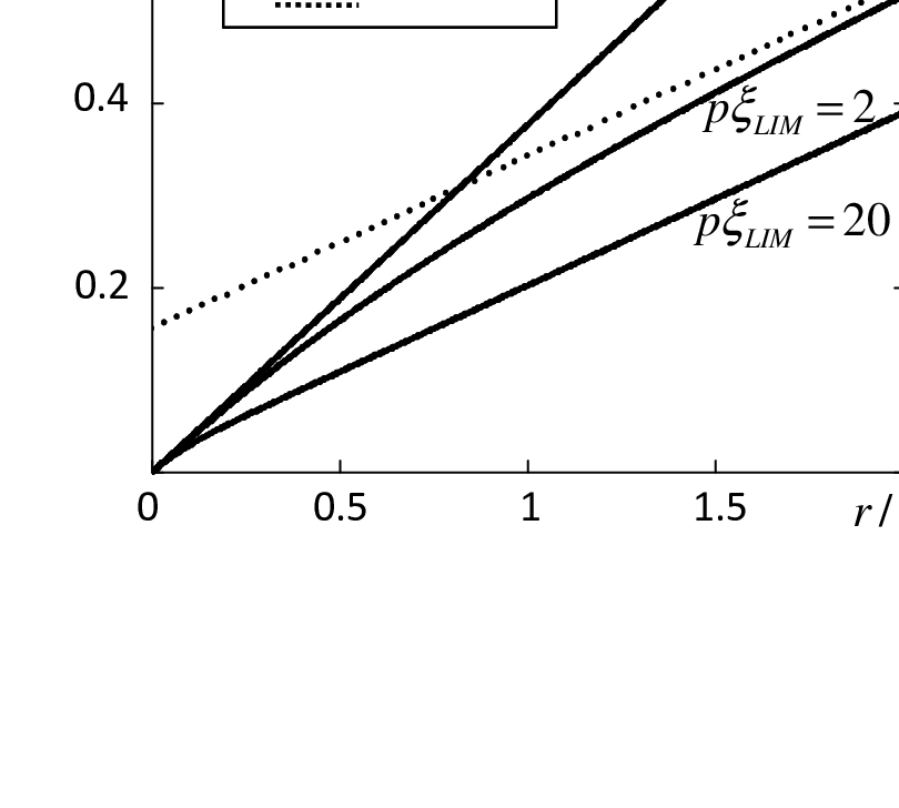
Figure 3: Dependence of ⟨(𝐥⁡(𝐫2)−𝐥⁡(𝐫1))2⟩/𝐥R2{\langle(\mathbf{l}(\mathbf{r}_{2})-\mathbf{l}(\mathbf{r}_{1}))^{2}\rangle}/{\mathbf{l}_{R}^{2}} on r/ξL​I​Mr/\xi_{LIM} for uniform stretching for three values of parameter p​ξL​I​M=0,2,20p\xi_{LIM}=0,~2,~20 and 𝐫|𝐰\mathbf{r}\|\mathbf{w}. Dotted line shows asymptotical dependence of correlator when r⋅p⟶∞r\cdot p\longrightarrow\infty. The upper solid line (p​ξL​I​M=0p\xi_{LIM}=0) is taken from Eq. 21.
Refer to caption
Figure 4: Dependence of ⟨(θ∥​(𝐫2)−θ∥​(𝐫1))2⟩\langle(\theta_{\|}(\mathbf{r}_{2})-\theta_{\|}(\mathbf{r}_{1}))^{2}\rangle on r/ξL​I​Mr/\xi_{LIM} for uniform stretching for three values of parameter p​ξL​I​M=0,0.25,10p\xi_{LIM}=0,~0.25,~10 and 𝐫|𝐰\mathbf{r}\|\mathbf{w}. Dotted line show asymptotical dependence of correlator when r⋅p⟶∞r\cdot p\longrightarrow\infty. The upper solid line (p​ξL​I​M=0p\xi_{LIM}=0) is taken from Eq. 22.

Solution of the equations (39)-(41) follows the same line as for the case κ<0\kappa<0. Essential difference is that now only one degree of freedom remains ”gapped”, it is rotation θu\theta_{u}, which takes 𝐥\mathbf{l} out of the u,vu,v plane. Two other rotations θv\theta_{v} and θw\theta_{w} move the triad 𝐦,𝐧,𝐥\mathbf{m},\mathbf{n},\mathbf{l} within its space of degeneracy. At a strong anisotropy 𝐥\mathbf{l} moves within the u,vu,v plane, but has random orientation within this plane. This state is referred as 2D LIM state[8].

Refer to caption
Figure 5: Dependence of ⟨(θu​(𝐫2)−θu​(𝐫1))2⟩\langle(\theta_{u}(\mathbf{r}_{2})-\theta_{u}(\mathbf{r}_{1}))^{2}\rangle on r/ξL​I​Mr/\xi_{LIM} for uniform stretching for four values of parameter p​ξL​I​M=0,0.5,1,2p\xi_{LIM}=0,~0.5,~1,~2 and 𝐫|𝐰\mathbf{r}\|\mathbf{w}. Dotted line show asymptotical dependence of correlator when r⋅p⟶∞r\cdot p\longrightarrow\infty.

The expressions for the correlators take a form of multiple integrals. We present here only results of numerical integration for the case when 𝐫|𝐰\mathbf{r}\|\mathbf{w} (FIG.3-5). Full expressions for integrals are given in Appendix C. In the region of r≪1/p{r}\ll 1/p the dependence of correlators on 𝐫\mathbf{r} is linear, for ⟨(𝐥⁡(𝐫2)−𝐥⁡(𝐫1))2⟩/𝐥R2{\langle(\mathbf{l}(\mathbf{r}_{2})-\mathbf{l}(\mathbf{r}_{1}))^{2}\rangle}/{\mathbf{l}_{R}^{2}} and ⟨(θ∥​(𝐫2)−θ∥​(𝐫1))2⟩\langle(\theta_{\|}(\mathbf{r}_{2})-\theta_{\|}(\mathbf{r}_{1}))^{2}\rangle it is given by Eqs. (19) and (20). The dependence of correlator ⟨(θu​(𝐫2)−θu​(𝐫1))2⟩\langle(\theta_{u}(\mathbf{r}_{2})-\theta_{u}(\mathbf{r}_{1}))^{2}\rangle in this region is close to 12​⟨(𝐥⁡(𝐫2)−𝐥⁡(𝐫1))2⟩/𝐥R2\frac{1}{2}{\langle(\mathbf{l}(\mathbf{r}_{2})-\mathbf{l}(\mathbf{r}_{1}))^{2}\rangle}/{\mathbf{l}_{R}^{2}}. In the opposite limit r≫1/p{r}\gg 1/p dependencies of the first two correlators can be approximated by the linear function ap​ξL​I​M+b⋅r\frac{a}{p\xi_{LIM}}+b\cdot r. The values of the coefficients aa and bb are given on the inserts on FIG. 3 and FIG. 4. The limiting value of ⟨(θu​(𝐫2)−θu​(𝐫1))2⟩\langle(\theta_{u}(\mathbf{r}_{2})-\theta_{u}(\mathbf{r}_{1}))^{2}\rangle at r​p≫1rp\gg 1 defines ⟨lw2⟩=12​⟨(θu​(𝐫2)−θu​(𝐫1))2⟩\langle l_{w}^{2}\rangle=\frac{1}{2}\langle(\theta_{u}(\mathbf{r}_{2})-\theta_{u}(\mathbf{r}_{1}))^{2}\rangle in linear regime, i.e. if p​ξL​I​M≫1p\xi_{LIM}\gg 1. It is found to be 0.31p​ξL​I​M\frac{0.31}{p\xi_{LIM}}, that is approximately half of the limiting value of correlator ⟨(𝐥⁡(𝐫2)−𝐥⁡(𝐫1))2⟩/𝐥R2{\langle(\mathbf{l}(\mathbf{r}_{2})-\mathbf{l}(\mathbf{r}_{1}))^{2}\rangle}/{\mathbf{l}_{R}^{2}} for the case of uniform compression (Eq. (33)).

IV Discussion

The approach, based on linearization of the equations of equilibrium is complementary to that, based on the argument of LIM. Linearized equations render a ”zoomed” picture of a small region within the LIM state or within the similar random textures of the order parameter of 3He-A in aerogel. Solutions of these equations present a quantitative description of a decrease of correlations of orientation of the order parameter and development of disorder with an increase of a distance between the two points within the chosen region. They describe also recovery of the long-range order when sufficiently strong global anisotropy is applied. In comparison with magnetic glasses the order parameter of 3He-A has additional degree of freedom – ”phase” variable. This variable is getting disordered together with the vector 𝐥\mathbf{l} although, unlike 𝐥\mathbf{l}, the ”phase” variable does not couple directly to the random anisotropy. Extrapolation of the results of linear analysis to distances of the order of ξL​I​M\xi_{LIM} matches the results based on the LIM argument. A qualitative picture obtained by such matching can be used as a guidance for a further quantitative description of random textures including the region r∼ξL​I​Mr\sim\xi_{LIM}, where nonlinearities become significant. That requires a serious numerical work, but it would render important results, e.g. a precise value of the critical global anisotropy, at which the phase transition from the disordered to the ordered state occurs, extension of the result for the NMR shift (Eq. (38)) in a region of finite fluctuations of the order parameter and description of global properties of textures, which can not be analyzed within the linear approximation.

V Acknowledgements

We thank V.V.Dmitriev for useful discussions and comments. This work was supported in part by the Russian Foundation for Basic Research, project # 14-02-00054-a and the Basic Research Program of the Presidium of Russian Academy of Sciences

Appendix A

In the linear approximation the superfluid velocity is determined by the gradient of θ∥​(𝐫)\theta_{\|}(\mathbf{r}): (vs)ξ=−ℏ2​m​∂θ∥∂xξ(v_{s})_{\xi}=-\frac{\hbar}{2m}\frac{\partial\theta_{\|}}{\partial x_{\xi}}. We are interested in the ensemble average

⟨vs2⟩=(ℏ2​m)2​⟨(∂θ∥∂r)2⟩,\langle v_{s}^{2}\rangle=\left(\frac{\hbar}{2m}\right)^{2}\left\langle\left(\frac{\partial\theta_{\|}}{\partial\textbf{r}}\right)^{2}\right\rangle, (42)

or in terms of Fourier components:

⟨vs2⟩=(ℏ2​m)2​∫k2​⟨θ∥​(𝐤)​θ∥​(−𝐤)⟩​V​d3​k(2​π)3\langle v_{s}^{2}\rangle=\left(\frac{\hbar}{2m}\right)^{2}\int k^{2}\langle\theta_{\|}(\mathbf{k})\theta_{\|}(-\mathbf{k})\rangle\frac{Vd^{3}k}{(2\pi)^{3}} (43)

with the aid of Eq. (15) ⟨vs2⟩\langle v_{s}^{2}\rangle can be expressed in terms of correlation functions of ηj​l​(𝐤)\eta_{jl}(\mathbf{k}). We assume that aerogel is globally isotropic, then ⟨ηx​z​(−𝐤)​ηy​z​(𝐤)⟩=0\langle\eta_{xz}(-\mathbf{k})\eta_{yz}(\mathbf{k})\rangle=0 and ⟨ηx​z​(−𝐤)​ηx​z​(𝐤)⟩=⟨ηy​z​(−𝐤)​ηy​z​(𝐤)⟩=K⁡(k)/V\langle\eta_{xz}(-\mathbf{k})\eta_{xz}(\mathbf{k})\rangle=\langle\eta_{yz}(-\mathbf{k})\eta_{yz}(\mathbf{k})\rangle=K(k)/V. With this assumption

⟨vs2⟩=(ℏ2​m)2​∫K⁡(k)​d3​k(2​π)3​ξs4​kz2​(k2−kz2)k2​(2​k2+kz2)2\langle v_{s}^{2}\rangle=\left(\frac{\hbar}{2m}\right)^{2}\int\frac{K(k)d^{3}k}{(2\pi)^{3}\xi_{s}^{4}}\frac{k_{z}^{2}(k^{2}-k_{z}^{2})}{k^{2}(2k^{2}+k_{z}^{2})^{2}} (44)

After integration over directions of 𝐤\mathbf{k} we arrive at:

⟨vs2⟩=(ℏ2​m)2​∫K⁡(k)​d​k(2​π)2​ξs4​I,\langle v_{s}^{2}\rangle=\left(\frac{\hbar}{2m}\right)^{2}\int\frac{K(k)dk}{(2\pi)^{2}\xi_{s}^{4}}I, (45)

where I=2​∫01d​u​u2​(1−u2)(2+u2)2=72​arccos⁡(23)−3≈0.05I=2\int_{0}^{1}du\frac{u^{2}(1-u^{2})}{(2+u^{2})^{2}}=\frac{7}{\sqrt{2}}\arccos(\sqrt{\frac{2}{3}})-3\approx 0.05. If the assumption K⁡(k)=c​o​n​s​tK(k)=const is used the integral over kk diverges linearly on the upper limit. For a crude estimation of the diverging integral we can cut it at k∼(1/ξc)k\sim(1/\xi_{c}) where the assumption K⁡(k)=c​o​n​s​tK(k)=const breaks down, then ⟨vs2⟩∼vF2​(a/ξs)2​(1−P)\langle v_{s}^{2}\rangle\sim v_{F}^{2}(a/\xi_{s})^{2}(1-P), here aa is interatomic distance. A more refined treatment is based on the fact that at distances of the order of ξc\xi_{c} aerogel has fractal dimensionality [23, 24] and at large kk K⁡(k)∼(1/kD)K(k)\sim(1/k^{D}) with D≃1.7−1.9D\simeq 1.7-1.9, then the integral converges [25], but the result depends on additional model assumptions or additional experimental data about the structure of aerogel.

Appendix B

Integrals from equations (17), (18) can be evaluated using cylindrical coordinates (kz,k⟂,φk_{z},~k_{\perp},~\varphi). Integration on kzk_{z} and then on φ\varphi yields zero-order Bessel function. The final expressions are the following:

⟨(𝐥⁡(𝐫2)−𝐥⁡(𝐫1))2⟩lR2=1ξL​I​M{172[z2+ρ2]12+\displaystyle\frac{\langle(\mathbf{l}(\mathbf{r}_{2})-\mathbf{l}(\mathbf{r}_{1}))^{2}\rangle}{l_{R}^{2}}=\frac{1}{\xi_{LIM}}\left\{\frac{17}{2}\left[z^{2}+\rho^{2}\right]^{\frac{1}{2}}+\right.
16​[z2+3​ρ2]12−10​63​[23​z2+ρ2]12−\displaystyle\left.\frac{1}{6}\left[z^{2}+3\rho^{2}\right]^{\frac{1}{2}}-\frac{10\sqrt{6}}{3}\left[\frac{2}{3}z^{2}+\rho^{2}\right]^{\frac{1}{2}}-\right.
16z∫0∞d​k⟂k⟂J0(k⟂ρ)sinh(1−232k⟂z)e−1+232​k⟂​z}\displaystyle\left.16z\int\limits_{0}^{\infty}\frac{dk_{\perp}}{k_{\perp}}J_{0}({k_{\perp}\rho})\sinh\left(\frac{1-\sqrt{\frac{2}{3}}}{2}k_{\perp}z\right)e^{-\frac{1+\sqrt{\frac{2}{3}}}{2}k_{\perp}z}\right\}
⟨(θ∥​(𝐫2)−θ∥​(𝐫1))2⟩=1ξL​I​M​(9​64​[23​z2+ρ2]12−CLOSE\displaystyle\langle(\theta_{\|}(\mathbf{r}_{2})-\theta_{\|}(\mathbf{r}_{1}))^{2}\rangle=\frac{1}{\xi_{LIM}}\left(\frac{9\sqrt{6}}{4}\left[\frac{2}{3}z^{2}+\rho^{2}\right]^{\frac{1}{2}}-\right.
112​[z2+ρ2]12+\displaystyle\frac{11}{2}\left[z^{2}+\rho^{2}\right]^{\frac{1}{2}}+
OPEN10​z​∫0∞d​k⟂k⟂​J0​(k⟂​ρ)​sinh⁡(1−232​k⟂​z)​e−1+232​k⟂​z)\displaystyle\left.10z\int\limits_{0}^{\infty}\frac{dk_{\perp}}{k_{\perp}}J_{0}({k_{\perp}\rho})\sinh\left(\frac{1-\sqrt{\frac{2}{3}}}{2}k_{\perp}z\right)e^{-\frac{1+\sqrt{\frac{2}{3}}}{2}k_{\perp}z}\right)

Evaluation of the integrals including Bessel functions for simple cases 𝐫|𝐳\mathbf{r}\|\mathbf{z} and 𝐫⟂𝐳\mathbf{r}\perp\mathbf{z} integrals with the Bessel function are evaluated and the final answers are given in the text above (Eqs. (19)-(22)).

Appendix C

Here we present expressions for correlators in a form of multiple integrals for the case of uniform stretching. The following shorthand notations are used: sin⁡α=sα\sin\alpha=s_{\alpha}, cos⁡α=cα\cos\alpha=c_{\alpha},

rw​(θ,φ,𝐫,p)=(x​sθ​cφ+y​sθ​sφ+z​cθ)​p,\displaystyle r_{w}(\theta,\varphi,\mathbf{r},p)=(xs_{\theta}c_{\varphi}+ys_{\theta}s_{\varphi}+zc_{\theta})p,
ε⁡(θ,φ)=(12​cφ2​s2​θ2+cθ2+2)1/2(2​cθ4+5​cθ2+2)1/2.\displaystyle\varepsilon(\theta,\varphi)=\frac{(\frac{1}{2}c^{2}_{\varphi}s_{2\theta}^{2}+c^{2}_{\theta}+2)^{1/2}}{(2c_{\theta}^{4}+5c_{\theta}^{2}+2)^{1/2}}.
⟨(𝐥⁡(𝐫)−𝐥⁡(0))2⟩lR2=1p​ξL​I​M​∫d​Ω4​π​A​(θ,φ,𝐫),\displaystyle\frac{\langle(\mathbf{l}(\mathbf{r})-\mathbf{l}(0))^{2}\rangle}{l_{R}^{2}}=\frac{1}{p\xi_{LIM}}\int\frac{d\Omega}{4\pi}A(\theta,\varphi,\mathbf{r}), (48)

where

A(θ,φ,𝐫)=12[1ε(1−(1−rwε)e−rw​ε)G1+\displaystyle A(\theta,\varphi,\mathbf{r})=\frac{1}{2}\left[\frac{1}{\varepsilon}\left(1-(1-r_{w}\varepsilon)e^{-r_{w}\varepsilon}\right)G_{1}+\right.
1ε3​(1−(1+rw​ε)​e−rw​ε)​G2−\displaystyle\frac{1}{\varepsilon^{3}}\left(1-(1+r_{w}\varepsilon)e^{-r_{w}\varepsilon}\right)G_{2}-
1ε5(3−2rwε−(3+rwε)e−rw​ε)G3],\displaystyle\left.\frac{1}{\varepsilon^{5}}\left(3-2r_{w}\varepsilon-(3+r_{w}\varepsilon)e^{-r_{w}\varepsilon}\right)G_{3}\right],
G1​(θ,φ)=2​(3−sθ4)2+sθ4​cθ4​(1+c2​φ2)+14​s2​φ2​sθ2​cθ2(2​cθ4+5​cθ2+2)2,\displaystyle G_{1}(\theta,\varphi)=\frac{2(3-s_{\theta}^{4})^{2}+s_{\theta}^{4}c_{\theta}^{4}(1+c^{2}_{2\varphi})+\frac{1}{4}s_{2\varphi}^{2}s_{\theta}^{2}c_{\theta}^{2}}{(2c_{\theta}^{4}+5c_{\theta}^{2}+2)^{2}},
G2​(θ,φ)=2​(1+sθ2)​(3−sθ4+c2​φ​sθ2​cθ2)(2​cθ4+5​cθ2+2)2,\displaystyle G_{2}(\theta,\varphi)=\frac{2(1+s_{\theta}^{2})(3-s_{\theta}^{4}+c_{2\varphi}s_{\theta}^{2}c_{\theta}^{2})}{(2c_{\theta}^{4}+5c_{\theta}^{2}+2)^{2}},
G3​(θ)=(1+sθ2)2(2​cθ4+5​cθ2+2)2.\displaystyle G_{3}(\theta)=\frac{(1+s_{\theta}^{2})^{2}}{(2c_{\theta}^{4}+5c_{\theta}^{2}+2)^{2}}.
⟨(θ∥​(𝐫)−θ∥​(0))2⟩=1p​ξL​I​M​∫d​Ω4​π​B​(θ,φ,𝐫)\displaystyle{\langle(\theta_{\|}(\mathbf{r})-\theta_{\|}(0))^{2}\rangle}=\frac{1}{p\xi_{LIM}}\int\frac{d\Omega}{4\pi}B(\theta,\varphi,\mathbf{r}) (49)
B(θ,φ,𝐫)=12[1ε(1−(1−rwε)e−rw​ε)H1+\displaystyle B(\theta,\varphi,\mathbf{r})=\frac{1}{2}\left[\frac{1}{\varepsilon}\left(1-(1-r_{w}\varepsilon)e^{-r_{w}\varepsilon}\right)H_{1}+\right.
1ε3​(1−(1+rw​ε)​e−rw​ε)​H2−\displaystyle\frac{1}{\varepsilon^{3}}\left(1-(1+r_{w}\varepsilon)e^{-r_{w}\varepsilon}\right)H_{2}-
1ε5(3−2rwε−(3+rwε)e−rw​ε)H3],\displaystyle\left.\frac{1}{\varepsilon^{5}}\left(3-2r_{w}\varepsilon-(3+r_{w}\varepsilon)e^{-r_{w}\varepsilon}\right)H_{3}\right],
H1​(θ)=sθ2​cθ2​(c2​θ+2)(2​cθ4+5​cθ2+2)2,\displaystyle H_{1}(\theta)=\frac{s_{\theta}^{2}c_{\theta}^{2}(c_{2\theta}+2)}{(2c_{\theta}^{4}+5c_{\theta}^{2}+2)^{2}},
H2​(θ,φ)=2​sθ2​cθ2​(c2​θ+2)​sφ2(2​cθ4+5​cθ2+2)2,\displaystyle H_{2}(\theta,\varphi)=\frac{2s_{\theta}^{2}c_{\theta}^{2}(c_{2\theta}+2)s_{\varphi}^{2}}{(2c_{\theta}^{4}+5c_{\theta}^{2}+2)^{2}},
H3​(θ,φ)=sθ2​cθ2​sφ2(2​cθ4+5​cθ2+2)2.\displaystyle H_{3}(\theta,\varphi)=\frac{s_{\theta}^{2}c_{\theta}^{2}s_{\varphi}^{2}}{(2c_{\theta}^{4}+5c_{\theta}^{2}+2)^{2}}.
⟨(θu​(𝐫)−θu​(0))2⟩=1p​ξL​I​M​∫d​Ω4​π​C​(θ,φ,𝐫)\displaystyle{\langle(\theta_{u}(\mathbf{r})-\theta_{u}(0))^{2}\rangle}=\frac{1}{p\xi_{LIM}}\int\frac{d\Omega}{4\pi}C(\theta,\varphi,\mathbf{r}) (50)
C⁡(θ,φ,𝐫)=12​[1ε​(1−(1−rw​ε)​e−rw​ε)​J],\displaystyle C(\theta,\varphi,\mathbf{r})=\frac{1}{2}\left[\frac{1}{\varepsilon}\left(1-(1-r_{w}\varepsilon)e^{-r_{w}\varepsilon}\right)J\right],
J⁡(θ,φ)=(3−sθ4+cθ2​sθ2​c2​φ)2+cθ4​sθ4​s2​φ2(2​cθ4+5​cθ2+2)2\displaystyle J(\theta,\varphi)=\frac{(3-s_{\theta}^{4}+c_{\theta}^{2}s_{\theta}^{2}c_{2\varphi})^{2}+c_{\theta}^{4}s_{\theta}^{4}s_{2\varphi}^{2}}{(2c_{\theta}^{4}+5c_{\theta}^{2}+2)^{2}}

References

  • [1] A. I. Larkin, Zh. Eksp. Teor. Fiz. 58, 1466 (1970), [Sov. Phys. JETP 31, 784 (1970)].
  • [2] Y. Imry and S. Ma, Phys. Rev. Lett. 35, 1399 (1975).
  • [3] E. M. Chudnovsky, W. M. Saslow, and R. A. Serota, Phys. Rev. B 33, 251 (1986).
  • [4] Y. Imry, J. Stat. Phys. 34, 849 (1984).
  • [5] D. Garanin and E. M. Chudnovsky, Eur. Phys. J. B 88, 81 (2015).
  • [6] T. C. Proctor and E. M. Chudnovsky, Phys. Rev. B 91, 140201 (2015).
  • [7] J. V. Porto and J. M. Parpia, Phys. Rev. Lett. 74, 4667 (1995).
  • [8] V.V.Dmitriev, D.A.Krasnikhin, N.Mulders, A.A.Senin, G.E.Volovik, and A.N.Yudin, Pis‘ma Zh. Eksp. Teor. Fiz. 91, 669 (2010), [JETP Lett. 91, 599 (2010)].
  • [9] G.E.Volovik, Pis‘ma Zh. Eksp. Teor. Fiz. 63, 301 (1996), [JETP Lett. 63, 301, (1996)].
  • [10] D. T. Sprague, T. M. Haard, J. B. Kycia, M. R. Rand, Y. Lee, P. J. Hamot, and W. P. Halperin, Phys. Rev. Lett. 75, 661 (1995).
  • [11] G. E. Volovik, J. Low Temp. Phys. 150, 453 (2008).
  • [12] I. A. Fomin, Pis’ma Zh. Eksp. Teor. Fiz. 104, 18 (2016), [JETP Lett. 104, 20 (2016)].
  • [13] I. A. Fomin, Journ. Phys. and Chem. of Solids 66, 1321 (2005).
  • [14] D. Vollhardt and P. Woelfle, The Superfluid Phases of Helium 3 (Tailor and Francis, London, New York, Phyladelphia, 1990).
  • [15] A. I. Larkin and Y. N. Ovchinnikov, Zh. Eksp. Teor. Fiz. 61, 1221 (1971), [Sov. Phys. JETP 34, 651 (1971)].
  • [16] E. V. Thuneberg, Quasiclassical methods in superconductivity and superfluidity, Verditz 96 , 53 (1998).
  • [17] E. V. Surovtsev and I. A. Fomin, J. Low Temp. Phys. 150, 487 (2008).
  • [18] D. Rainer and M. Vuorio, J. Phys. C: Solid State Phys. 10, 3093 (1977).
  • [19] T. Kunimatsu, T. Sato, K. Izumina, A. Matsubara, Y. Sasaki, M. Kubota, O. Ishikawa, T. Mizusaki, and Y. M. Bunkov, Pis’ma Zh. Eksp. Teor. Fiz. 86, 244 (2007), [JETP Lett. 86, 216 (2007)].
  • [20] I. A. Fomin and E. V. Surovtsev, Phys. Rev. B 92, 064509 (2015).
  • [21] J. Elbs, Y. M. Bunkov, E. Collin, H. Godfrin, and G. E. Volovik, Phys. Rev. Lett. 100, 215304 (2008).
  • [22] J. I. A. Li, A. M. Zimmerman, J. Pollanen, C. A. Collett, W. J. Gannon, and W. P. Halperin, J. Low Temp. Phys. 175, 31 (2013).
  • [23] J. V. Porto and J. M. Parpia, Phys. Rev. B 59, 14583 (1999).
  • [24] W. P. Halperin, H. Choi, J. P. Davis, and J. Polanen, J. Phys. Soc. Jpn. 77, 111002 (2008).
  • [25] I. A. Fomin, Pis’ma Zh. Eksp. Teor. Fiz. 88, 65 (2008), [JETP Lett. 88, 59 (2008)].