Physical implications of symmetry in exact solutions for a self-repressing gene
Abstract
We chemically characterize the symmetries underlying the exact solutions of a stochastic negatively self-regulating gene. The breaking of symmetry at low molecular number causes three effects. Two branches of the solution exist, having high and low switching rates, such that the low switching rate branch approaches deterministic behavior and the high switching rate branch exhibits sub-Fano behavior. Average protein number differs from the deterministically expected value. Bimodal probability distributions appear as the protein number becomes a readout of the ON/OFF state of the gene.
Keywords:
Lie symmetries; Stochastic gene regulationpacs
87.10.Mn, 87.10.Ca, 87.16.Yc, 87.18.Tt, 02.20.Sv, 02.30.Gp, 02.50.Eytoday
Symmetries, described by Lie algebras, have been central tools for new discoveries in quantum mechanics and quantum field theory [1, 2, 3]. Applications of these techniques to problems in statistical physics have been limited [4, 5]. Over the last two decades, statistical physics has been widely applied to biological systems [6]. Such studies frequently make use of the chemical master equation (CME), typically solved by Gillespie’s direct simulation method [7]. This method requires reconstructing probability distributions experimentally from repeated computational runs, a procedure that can overlook important features of the distributions. In a case where exact solutions were obtained to the CME for a self-repressing gene [8] in terms of generating functions with a symmetry described by a Lie algebra [9], physical insight into the general behavior of the system was limited by the dimensionality of the parameter space and the lack of a physical interpretation of the symmetry. In this paper, we show that this symmetry has three important physical effects. First, an invariant quantity under the group’s action is a quadratic function of a certain ratio of protein removal rates. The two roots of that quadratic induce two branches of the solution. One branch approaches a deterministic regime as molecular number increases, while the other represents a novel class of stochastic behavior. Second, symmetry in the form of numerical equivalence between the average number of molecules in the system in the deterministic and stochastic regimes is lost when molecular number becomes sufficiently small. Finally, actions of the group that leave the system unchanged in the deterministic limit have two completely distinct effects in the stochastic regime depending on whether the system can be defined by a Langevin approximation or not. These physical manifestations of the underlying symmetry also provide a systematic characterization of the model’s behavior in the entire parameter space of the exact solutions. This mathematical characterization has previously been reported by use of the Poisson representation [14, 15]. The analysis of symmetries reveals new phenomenology in a fundamental physical system for investigating gene networks. The use of group theoretical techniques on generating functions represents a new class of applications of this technique for related problems involving the CME [10, 11] and other applications [12, 13]. It has provided us with a way to identify the building blocks necessary to understand the workings of randomness and invariance in biological systems.
We conceive a deterministic model for a negative self-regulating gene as an ensemble of genes (operators, in the case of a prokaryote) at concentration . The operators may be in the ON or OFF state if they are, respectively, unbound or bound to the regulatory protein. The concentration of ON (OFF) operators is indicated by (), with , and the protein concentration is given by . The macroscopic reaction scheme is given by
|
(1) |
All macroscopic rate constants are written with hats. and each have units of minute-1, while has units of liter/minute. (1) implies that
We denote the steady state concentrations of and by and Then
| (2) | |||||
| (3) |
where , the equilibrium affinity, is given by liters, and . Eq. (2) indicates that the rate at which operators move from OFF to ON and ON to OFF is, respectively, given by and . Thus, the total rate of operator switching in both directions is . Note that the expected concentration of proteins is given by the product of the ratio between the protein synthesis and degradation rates and the concentration of ON operators. Hence, at the limit of small affinity of the repressor for the operator (), , the expected number of proteins in the absence of regulation.
A stochastic model for the negative self-regulating gene has been proposed in terms of two random variables, the protein number, denoted by , and the operator state, which can be ON or OFF [8]. The steady state probability of finding proteins and the operator ON or OFF is denoted by or , respectively. In the stochastic model, we replace the reaction rate constants of Eq. (1) by propensities represented by the unhatted symbols and where is the system volume [7]. Note that now we may consider a single gene instead of an ensemble and the proportion of ON operators of the deterministic model becomes the marginal probability of finding the operator ON, . The marginal probability of finding proteins in the cytoplasm independently of the operator state being ON or OFF is given by and is computed in terms of the KummerM functions, so that
where denotes the Pochhammer symbol defined by and , and
| (4) | |||
is the average number of proteins at the steady state regime if the operator is fully ON. gives the proportion of protein removal from cytoplasm by first order decay. is the ratio of the OFF to ON transition rate to the protein degradation rate. () indicates a regime where, on average, the OFF operator switches back to the ON state faster (slower) than the time required for protein degradation. gives the ratio of the operator switching to the protein removal rates. The operator switching rate is the sum of the average OFF to ON switching rate and the ON to OFF rate defined in analogy with the deterministic case to be . For the operator switches multiple times between the ON and OFF states during the average time for protein removal. In that case, the probability distributions for protein number are unimodal. On average, for or smaller, the operator takes longer to switch from ON to OFF to ON (or vice-versa) than the average protein removal time. In that case, and for , the probability distributions for protein number are bimodal because most of the proteins synthesized when the operator is ON decay before the operator switches OFF. The average protein number of the distribution is given by
which can be written as , with the stochastic equivalent of in Eq. (3).
This stochastic model is a combination of two stochastic processes, and hence approaches equilibrium at the two rates and , the former related to the protein degradation and the latter to operator switching [16]. The smallest of those two rates determine when the system reaches equilibrium. The time dependent solutions in terms of generating functions has the form
| (5) |
where is a non-negative integer and and are confluent Heun functions [16, 17]. These solutions are obtained applying the separability ansatz whose component obeys a second-order ODE having two regular poles, one around , giving , and the other around , giving . It is evident that the only steady state solutions in Eq. (5) have vanishing time dependent exponents, implying the selection of and . can then be written as a a KummerM function, so that
| (6) |
is the generating function of the probabilities .
These exact solutions of the steady state stochastic model indicated the existence of symmetries [9]. The generating functions in Eq (6) span irreducible representations of , which in the Cartan basis has its operators denoted by and . The Casimir operator is defined as and the commutation relations are
The action of the algebraic operators on the generating functions is:
| (7) | |||
| (8) | |||
| (9) |
The invariant of the algebra is determined by the eigenvalue of the Casimir operator and Eq. (7) implies that is constant. The Cartan operator’s eigenvalue in Eq. (8) determines the OFF to ON switching rate in relation to the protein degradation rate, while the ladder operators change the value of by one.


We start building the biological interpretation of the symmetries of the model by writing its invariant as . A fixed leads to a 3D locus embedded in a 4D space. For fixed values of we obtain two possible values for , given by
| (10) |
FIG 1A shows the possible values of as functions of . implies which is biologically meaningless and only has acceptable values (Eq. 4). For a given the dynamical regime of the system is degenerate and two values of distinguish those regimes in terms of the ON to OFF operator state transition. The first regime, (), has strong self-repression (high value of ) and low steady state protein number. The second regime, (), is characterized by a high steady state protein number and weak self-repression (low value of ).
FIG 1B shows a further consequence of this degeneracy on the average protein number. For sufficiently low , one has two possible values of and , both characterized by the same value of . Those values indicate two regimes of operator switching, with lower (or higher) values for the switching rates and , that is, slow or fast switching. For the specific condition when one regime has and the other has the noise on the protein numbers is characterized, respectively, as sub-Fano and super-Fano.

The stochastic model exhibits splitting between the deterministic and stochastic solutions to the dynamics of the negative self-regulating gene when the average protein numbers are low. FIG 2A shows a comparison between the steady state concentration of proteins predicted by the deterministic model in Eq. (3) and the average protein number as given by the stochastic model. For high values of there is a good agreement for the steady state number of proteins predicted by both the stochastic and deterministic approaches. As the steady state number of proteins decreases, discrepancies between the two approaches start to appear as . For sufficiently high, the probability for the gene being OFF increases and when becomes very small the stochastic and deterministic solutions diverge. The correspondence principle breaks down when the molecular number is extremely small. FIG 2A shows that for , large values of cause the protein number to approach . This is a consequence of the fact that a protein bound to the operator does not decay in the reaction scheme given in Eq (1), and we have shown elsewhere that this case can give rise to Fano factors arbitrarily close to zero [18].


A third type of splitting arises from the following. The parameter is the eigenvalue of the Cartan operator and gives the OFF to ON transition rate (see Eq. (8)). The action of the ladder operators on the probability generating function changes the value of by one (Eq. (9)) and connects probability distributions in which values are the same and values differ by an integer. The action of the raising operator changes to , and the action of is constructed by analogy. Let us assume that the action of only changes , hence and . remains unchanged under the action of , hence the remaining constants and change. For a fixed value of one has . For a fixed value of we consider that with . The increment of (or ) corresponds to an decrease (or increase) of the value of that implies an increase of the mean protein number (see FIG 3B).
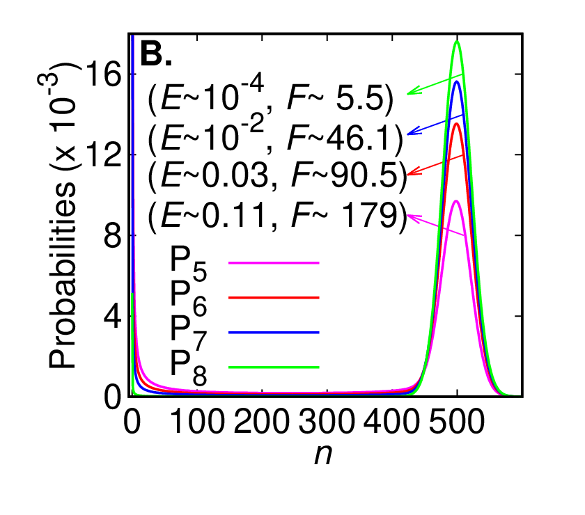
The dynamics of the gene expression process may have two distinct characteristics, depending on the value of . For the dominant decay rate to equilibrium is and the changes of the value of are not sufficient to cause changes in the time for the system to approach equilibrium, . This regime coincides with a unimodal probability distribution and the action of the raising operator on the generating functions causes the mode of its probability distribution to be displaced to the right. For the case of (or ) we have that is the dominant decay rate and the increase (or decrease) of corresponds to the system reaching equilibrium earlier (or later). This regime is characterized by probability distributions that may become bimodal and the action of the raising operator corresponds to an increase of the maximum probability of finding equal to the higher mode (see FIGs 3A and 2B).
The regime with bimodal distributions has important experimental and theoretical consequences. In this regime, most of the proteins synthesized by the gene during the ON state are degraded before it switches back to the OFF state, and the remaining proteins degrade before the gene switches ON, giving rise to bimodal distributions of which have been experimentally observed [19]. In that case, the assumptions underlying the Langevin approach fail [20] because the number of proteins at the steady state regime of the Langevin equation is governed by distributions that are Gaussian around . The probability distributions in this case and the breakdown of the Langevin regime are shown in FIG 2B.
We began our treatment by considering the macroscopic system because the master equation solution applies to cases with any number of molecules. This point is demonstrated by FIG 2A, which shows that increasing the equilibrium binding affinity reduces the deterministic equilibrium concentration, as expected. For fixed , reducing requires reducing . FIG 2A shows that there is a symmetry breaking as the average protein number in the deterministic model splits from that given by the stochastic model, and moreover that the average number of proteins in the stochastic model is a function of even when is held constant, behavior never seen in the deterministic model. Although the deterministic correspondence principle holds for small numbers of molecules (), correspondence is lost at one repressor molecule per cell, as discussed above.
The kinetic symmetries fully manifest themselves in the macroscopic case. The invariant of the algebra, is the ratio between the switching rate and the protein removal rate. Since the invariant is quadratic in , there exist two kinetic regimes for the same value of . The first has protein removal predominantly because of protein destruction (for example, when ) while protein binding prevails in the second. These regimes are macroscopically indistinguishable in the presence of a thermodynamically large number of operator sites. This fully macroscopic picture in fact never occurs in a biological system, because the molecular number of operator sites per cell is small. In the “semi-macroscopic” case of many protein molecules and a small number of operator sites, corresponding to the branch in FIG 1A,B, protein removal takes place primarily by first order decay. This super-Fano regime approaches the solutions of a near equilibrium thermodynamic system as molecular number increases. In the branch, protein removal takes place primarily by binding, the operator becomes strongly repressed, and sub-Fano behavior results, a situation we have discussed in detail elsewhere [18].
A further symmetry breaking manifests itself for certain values of with respect to the protein number distribution when the number of operators is small. For the case of the gene switching is slow in comparison with the protein removal rate, hence the probability distributions for the protein number when the gene is ON (or OFF) are split, and bimodal probability distributions are observed (see FIGs 3A and 2B). When the operator number is large, these differences in ON and OFF states would average out in the reaction mixture and become unobservable. Here the actual biological regime of small gene number per cell is experimentally significant because it permits direct observation of stochastic switching between ON and OFF in living cells [19]. When the gene switching is fast in comparison with protein removal rate () the distributions are unimodal and the existence of the two gene states cannot be established by the measurement of protein numbers, even with low gene copy number (see FIG 3B).
In conclusion, we have made use of symmetries described by a Lie algebra to fully characterize the behavior of a self-repressing gene. Because the exact solutions represent the behavior of the system for any number of reacting molecules and all values of kinetic constants, we interpret the deviation from deterministic behavior, the splitting of the two branches of , and the emergence of bimodal protein distributions as different types of symmetry breaking. The role the symmetries play in this analysis differs from how they are used in quantum problems, where symmetries involve the quantum state directly. Deeper insight into the role of symmetries will be helpful not only to statistical physics, but also to other areas involving stochastic processes, including biological evolution [12, 13].
Acknowledgements.
AFR was supported by CAPES (88881.062174/2014-01). JR was supported by NIH R01 OD010936. We thank UnJin Lee and David H. Sharp for helpful comments, and J. E. M. Hornos for stimulating discussion.References
- [1] P. W. Anderson. Coherent excited states in the theory of superconductivity: Gauge invariance and the Meissner effect. Phys. Rev., 110:827–835, 1958.
- [2] M. Gell-Mann and Y. Ne’eman. The eightfold way. Benjamin, New York, 1964.
- [3] P. W. Higgs. Broken symmetries and the masses of gauge bosons. Phys. Rev. Lett., 13:508, 1964.
- [4] L. Cannavacciuolo and J. Hulliger. Polarity formation in molecular crystals as a symmetry breaking effect. Symmetry, 8:10, 2016.
- [5] M. Tamm. A combinatorial approach to time asymmetry. Symmetry, 8:11, 2016.
- [6] A. Arkin, J. Ross, and H. H. MacAdams. Stochastic kinetic analysis of developmental pathway bifurcation in phage -infected Escherichia coli cells. Genetics, 149:1633–1648, 1998.
- [7] D. T. Gillespie. Exact stochastic simulation of coupled chemical reactions. J Phys Chem, 81:2340–2361, 1977.
- [8] J. E. M. Hornos, D. Schultz, G. C. P. Innocentini, J. Wang et al. Self-regulating gene: an exact solution. Phys Rev E, 72:051907, 2005.
- [9] A. F. Ramos and J. E. M. Hornos. Symmetry and stochastic gene regulation. Phys Rev Lett, 99:108103, 2007.
- [10] G. C. P. Innocentini and J. E. M. Hornos. Modeling stochastic gene expression under repression. J Math Biol, 55(3):413–31, 2007.
- [11] D. Lepzelter and J. Wang. Exact probabilistic solution of spatial-dependent stochastics and associated spatial potential landscape for the bicoid protein. Phys Rev E, 77:041917, 2008.
- [12] J. E. M. Hornos and Y. M. M. Hornos. Algebraic model for the evolution of the genetic code. Phys Rev Lett, 71(26):4401–4404, 1993.
- [13] J. D. Bashford, P. D. Jarvis, J. G. Sumner, and M. A. Steel. U(1)U(1)U(1) symmetry of the kimura 3st model and phylogenetic branching processes. J Phys A, 37:L81–L89, 2004.
- [14] C. W. Gardiner and S. Chaturvedi The Poisson representation. I. A new technique for chemical master equations. J Stat Phys, 17(6):429–468, 1977.
- [15] S. Iyer-Biswas and C. Jayaprakash Mixed Poisson distributions in exact solutions of stochastic autoregulation models. Phys Rev E, 90:052712, 2014
- [16] A. F. Ramos, G. C. P. Innocentini and J. E. M. Hornos. Exact time-dependent solutions for a self-regulating gene. Phys Rev E, 83:062902, 2011.
- [17] A. Ronveaux. Heun’s Differential Equations. Oxford University Press, 1995.
- [18] A. F. Ramos, J. E. M. Hornos, and J. Reinitz Gene regulation and noise reduction by coupling of stochastic processes. Phys Rev E, 91:020701(R), 2015.
- [19] D. M. Suter, N. Molina, D. Garfield, K. Schneider, U. Schibler, and F. Naef. Mammalian genes are transcribed with widely different bursting kinetics. Science, 332:472–474, 2011.
- [20] D. T. Gillespie. The chemical Langevin equation. J Chem Phys, 113:297–306, 2000.