Deep Learning with Topological Signatures
Abstract
Inferring topological and geometrical information from data can offer an alternative perspective on machine learning problems. Methods from topological data analysis, e.g., persistent homology, enable us to obtain such information, typically in the form of summary representations of topological features. However, such topological signatures often come with an unusual structure (e.g., multisets of intervals) that is highly impractical for most machine learning techniques. While many strategies have been proposed to map these topological signatures into machine learning compatible representations, they suffer from being agnostic to the target learning task. In contrast, we propose a technique that enables us to input topological signatures to deep neural networks and learn a task-optimal representation during training. Our approach is realized as a novel input layer with favorable theoretical properties. Classification experiments on 2D object shapes and social network graphs demonstrate the versatility of the approach and, in case of the latter, we even outperform the state-of-the-art by a large margin.
1 Introduction
Methods from algebraic topology have only recently emerged in the machine learning community, most prominently under the term topological data analysis (TDA) [7]. Since TDA enables us to infer relevant topological and geometrical information from data, it can offer a novel and potentially beneficial perspective on various machine learning problems. Two compelling benefits of TDA are (1) its versatility, i.e., we are not restricted to any particular kind of data (such as images, sensor measurements, time-series, graphs, etc.) and (2) its robustness to noise. Several works have demonstrated that TDA can be beneficial in a diverse set of problems, such as studying the manifold of natural image patches [8], analyzing activity patterns of the visual cortex [28], classification of 3D surface meshes [27, 22], clustering [11], or recognition of 2D object shapes [29].
Currently, the most widely-used tool from TDA is persistent homology [15, 14]. Essentially11 1 We will make these concepts more concrete in Sec. 2., persistent homology allows us to track topological changes as we analyze data at multiple “scales”. As the scale changes, topological features (such as connected components, holes, etc.) appear and disappear. Persistent homology associates a lifespan to these features in the form of a birth and a death time. The collection of (birth, death) tuples forms a multiset that can be visualized as a persistence diagram or a barcode, also referred to as a topological signature of the data. However, leveraging these signatures for learning purposes poses considerable challenges, mostly due to their unusual structure as a multiset. While there exist suitable metrics to compare signatures (e.g., the Wasserstein metric), they are highly impractical for learning, as they require solving optimal matching problems.
Related work. In order to deal with these issues, several strategies have been proposed. In [2] for instance, Adcock et al. use invariant theory to “coordinatize” the space of barcodes. This allows to map barcodes to vectors of fixed size which can then be fed to standard machine learning techniques, such as support vector machines (SVMs). Alternatively, Adams et al. [1] map barcodes to so-called persistence images which, upon discretization, can also be interpreted as vectors and used with standard learning techniques. Along another line of research, Bubenik [6] proposes a mapping of barcodes into a Banach space. This has been shown to be particularly viable in a statistical context (see, e.g., [10]). The mapping outputs a representation referred to as a persistence landscape. Interestingly, under a specific choice of parameters, barcodes are mapped into and the inner-product in that space can be used to construct a valid kernel function. Similar, kernel-based techniques, have also recently been studied by Reininghaus et al. [27], Kwitt et al. [20] and Kusano et al. [19].
While all previously mentioned approaches retain certain stability properties of the original representation with respect to common metrics in TDA (such as the Wasserstein or Bottleneck distances), they also share one common drawback: the mapping of topological signatures to a representation that is compatible with existing learning techniques is pre-defined. Consequently, it is fixed and therefore agnostic to any specific learning task. This is clearly suboptimal, as the eminent success of deep neural networks (e.g., [18, 17]) has shown that learning representations is a preferable approach. Furthermore, techniques based on kernels [27, 20, 19] for instance, additionally suffer scalability issues, as training typically scales poorly with the number of samples (e.g., roughly cubic in case of kernel-SVMs). In the spirit of end-to-end training, we therefore aim for an approach that allows to learn a task-optimal representation of topological signatures. We additionally remark that, e.g., Qi et al. [25] or Ravanbakhsh et al. [26] have proposed architectures that can handle sets, but only with fixed size. In our context, this is impractical as the capability of handling sets with varying cardinality is a requirement to handle persistent homology in a machine learning setting.
Contribution. To realize this idea, we advocate a novel input layer for deep neural networks that takes a topological signature (in our case, a persistence diagram), and computes a parametrized projection that can be learned during network training. Specifically, this layer is designed such that its output is stable with respect to the 1-Wasserstein distance (similar to [27] or [1]). To demonstrate the versatility of this approach, we present experiments on 2D object shape classification and the classification of social network graphs. On the latter, we improve the state-of-the-art by a large margin, clearly demonstrating the power of combining TDA with deep learning in this context.
2 Background
For space reasons, we only provide a brief overview of the concepts that are relevant to this work and refer the reader to [16] or [14] for further details.
Homology. The key concept of homology theory is to study the properties of some object by means of (commutative) algebra. In particular, we assign to a sequence of modules which are connected by homomorphisms such that . A structure of this form is called a chain complex and by studying its homology groups we can derive properties of .
A prominent example of a homology theory is simplicial homology. Throughout this work, it is the used homology theory and hence we will now concretize the already presented ideas. Let be a simplicial complex and its -skeleton. Then we set as the vector space generated (freely) by over 22 2 Simplicial homology is not specific to , but it’s a typical choice, since it allows us to interpret -chains as sets of -simplices.. The connecting homomorphisms are called boundary operators. For a simplex , we define them as and linearly extend this to , i.e., . Persistent homology. Let be a simplicial complex and a sequence of simplicial complexes such that . Then, is called a filtration of . If we use the extra information provided by the filtration of , we obtain the following sequence of chain complexes (left),
where and denotes the inclusion. This then leads to the concept of persistent homology groups, defined by
The ranks, , of these homology groups (i.e., the -th persistent Betti numbers), capture the number of homological features of dimensionality (e.g., connected components for , holes for , etc.) that persist from to (at least) . In fact, according to [14, Fundamental Lemma of Persistent Homology], the quantities
| (1) |
encode all the information about the persistent Betti numbers of dimension .
Topological signatures. A typical way to obtain a filtration of is to consider sublevel sets of a function . This function can be easily lifted to higher-dimensional chain groups of by
Given , we obtain by setting and for , where is the sorted sequence of values of . If we construct a multiset such that, for , the point is inserted with multiplicity , we effectively encode the persistent homology of dimension w.r.t. the sublevel set filtration induced by . Upon adding diagonal points with infinite multiplicity, we obtain the following structure:
Definition 1 (Persistence diagram).
Let be the multiset of the diagonal , where mult denotes the multiplicity function and let . A persistence diagram, , is a multiset of the form
We denote by the set of all persistence diagrams of the form
For a given complex of dimension and a function (of the discussed form), we can interpret persistent homology as a mapping , where is the diagram of dimension and the dimension of . We can additionally add a metric structure to the space of persistence diagrams by introducing the notion of distances.
Definition 2 (Bottleneck, Wasserstein distance).
For two persistence diagrams and , we define their Bottleneck () and Wasserstein () distances by
| (2) |
where and the infimum is taken over all bijections .
3 A network layer for topological signatures
In this section, we introduce the proposed (parametrized) network layer for topological signatures (in the form of persistence diagrams). The key idea is to take any and define a projection w.r.t. a collection (of fixed size ) of structure elements.
In the following, we set and , resp., and start by rotating points of such that points on lie on the -axis, see Fig. 1. The -axis can then be interpreted as the persistence of features. Formally, we let and be the unit vectors in directions and and define a mapping such that . This rotates points in clock-wise by . We will later see that this construction is beneficial for a closer analysis of the layers’ properties. Similar to [27, 19], we choose exponential functions as structure elements, but other choices are possible (see Lemma 1). Differently to [27, 19], however, our structure elements are not at fixed locations (i.e., one element per point in ), but their locations and scales are learned during training.
Definition 3.
Let and . We define
as follows:
| (3) |
A persistence diagram is then projected w.r.t. via
| (4) |
Remark.
Note that is continuous in as
and is continuous. Further, is differentiable on , since
Also note that we use the log-transform in Eq. (4) to guarantee that satisfies the conditions of Lemma 1; this is, however, only one possible choice. Finally, given a collection of structure elements , we combine them to form the output of the network layer.
Definition 4.
Importantly, a network layer implementing Def. 4 is trainable via backpropagation, as (1) is differentiable in , (2) is a finite sum of and (3) is just a concatenation.
4 Theoretical properties
In this section, we demonstrate that the proposed layer is stable w.r.t. the 1-Wasserstein distance , see Eq. (2). In fact, this claim will follow from a more general result, stating sufficient conditions on functions such that a construction in the form of Eq. (3) is stable w.r.t. .
Lemma 1.
Let
have the following properties:
- (i)
is Lipschitz continuous w.r.t. and constant
- (ii)
, for
Then, for two persistence diagrams , it holds that
| (5) |
Proof.
see Appendix B ∎
Remark.
At this point, we want to clarify that Lemma 1 is not specific to (e.g., as in Def. 3). Rather, Lemma 1 yields sufficient conditions to construct a -stable input layer. Our choice of is just a natural example that fulfils those requirements and, hence, is just one possible representative of a whole family of input layers.
With the result of Lemma 1 in mind, we turn to the specific case of and analyze its stability properties w.r.t. . The following lemma is important in this context.
Lemma 2.
has absolutely bounded first-order partial derivatives w.r.t. and on .
Proof.
see Appendix B ∎
Theorem 1.
is Lipschitz continuous with respect to on .
Proof.
Lemma 2 immediately implies that from Eq. (3) is Lipschitz continuous w.r.t . Consequently, satisfies property (i) from Lemma 1; property (ii) from Lemma 1 is satisfied by construction. Hence, is Lipschitz continuous w.r.t. . Consequently, is Lipschitz in each coordinate and therefore Liptschitz continuous. ∎
Interestingly, the stability result of Theorem 1 is comparable to the stability results in [1] or [27] (which are also w.r.t. and in the setting of diagrams with finitely-many points). However, contrary to previous works, if we would chop-off the input layer after network training, we would then have a mapping of persistence diagrams that is specifically-tailored to the learning task on which the network was trained.
5 Experiments
To demonstrate the versatility of the proposed approach, we present experiments with two totally different types of data: (1) 2D shapes of objects, represented as binary images and (2) social network graphs, given by their adjacency matrix. In both cases, the learning task is classification. In each experiment we ensured a balanced group size (per label) and used a 90/10 random training/test split; all reported results are averaged over five runs with fixed . In practice, points in input diagrams were thresholded at for computational reasons. Additionally, we conducted a reference experiment on all datasets using simple vectorization (see Sec. 5.3) of the persistence diagrams in combination with a linear SVM.
Implementation. All experiments were implemented in PyTorch33 3 https://github.com/pytorch/pytorch, using DIPHA44 4 https://bitbucket.org/dipha/dipha and Perseus [23]. Source code is publicly-available at https://github.com/c-hofer/nips2017.
5.1 Classification of 2D object shapes

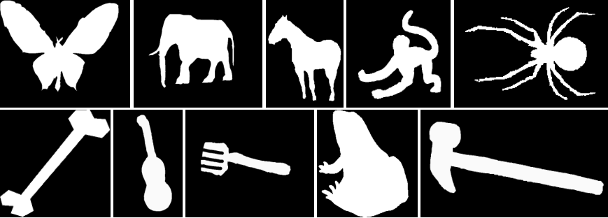
We apply persistent homology combined with our proposed input layer to two different datasets of binary 2D object shapes: (1) the Animal dataset, introduced in [3] which consists of 20 different animal classes, 100 samples each; (2) the MPEG-7 dataset which consists of 70 classes of different object/animal contours, 20 samples each (see [21] for more details).
Filtration. The requirements to use persistent homology on 2D shapes are twofold: First, we need to assign a simplicial complex to each shape; second, we need to appropriately filtrate the complex. While, in principle, we could analyze contour features, such as curvature, and choose a sublevel set filtration based on that, such a strategy requires substantial preprocessing of the discrete data (e.g., smoothing). Instead, we choose to work with the raw pixel data and leverage the persistent homology transform, introduced by Turner et al. [29]. The filtration in that case is based on sublevel sets of the height function, computed from multiple directions (see Fig. 2). Practically, this means that we directly construct a simplicial complex from the binary image. We set as the set of all pixels which are contained in the object. Then, a 1-simplex is in the 1-skeleton iff and are 4–neighbors on the pixel grid. To filtrate the constructed complex, we define by the barycenter of the object and with the radius of its bounding circle around . Finally, we define, for and , the filtration function by . Function values are lifted to by taking the maximum, cf. Sec. 2. Finally, let be the 32 equidistantly distributed directions in , starting from . For each shape, we get a vector of persistence diagrams where is the 0-th diagram obtained by filtration along . As most objects do not differ in homology groups of higher dimensions (> 0), we did not use the corresponding persistence diagrams.
Network architecture. While the full network is listed in the supplementary material (Fig. 6), the key architectural choices are: independent input branches, i.e., one for each filtration direction. Further, the -th branch gets, as input, the vector of persistence diagrams from directions and . This is a straightforward approach to capture dependencies among the filtration directions. We use cross-entropy loss to train the network for epochs, using stochastic gradient descent (SGD) with mini-batches of size and an initial learning rate of (halved every -th epoch). Results. Fig. 3 shows a selection of 2D object shapes from both datasets, together with the obtained classification results. We list the two best () and two worst () results as reported in [30]. While, on the one hand, using topological signatures is below the state-of-the-art, the proposed architecture is still better than other approaches that are specifically tailored to the problem. Most notably, our approach does not require any specific data preprocessing, whereas all other competitors listed in Fig. 3 require, e.g., some sort of contour extraction. Furthermore, the proposed architecture readily generalizes to 3D with the only difference that in this case . Fig. 4 (Right) shows an exemplary visualization of the position of the learned structure elements for the Animal dataset.
5.2 Classification of social network graphs
| MPEG-7 | Animal | |
|---|---|---|
| ‡Skeleton paths | ||
| ‡Class segment sets | ||
| †ICS | ||
| †BCF | ||
| Ours |
In this experiment, we consider the problem of graph classification, where vertices are unlabeled and edges are undirected. That is, a graph is given by , where denotes the set of vertices and denotes the set of edges. We evaluate our approach on the challenging problem of social network classification, using the two largest benchmark datasets from [31], i.e., reddit-5k (5 classes, 5k graphs) and reddit-12k (11 classes, 12k graphs). Each sample in these datasets represents a discussion graph and the classes indicate subreddits (e.g., worldnews, video, etc.).
Filtration. The construction of a simplicial complex from is straightforward: we set and . We choose a very simple filtration based on the vertex degree, i.e., the number of incident edges to a vertex . Hence, for we get and again lift to by taking the maximum. Note that chain groups are trivial for dimension , hence, all features in dimension are essential.
Network architecture. Our network has four input branches: two for each dimension ( and ) of the homological features, split into essential and non-essential ones, see Sec. 2. We train the network for epochs using SGD and cross-entropy loss with an initial learning rate of (reddit_5k), or (reddit_12k). The full network architecture is listed in the supplementary material (Fig. 7).
Results. Fig. 5 (right) compares our proposed strategy to state-of-the-art approaches from the literature. In particular, we compare against (1) the graphlet kernel (GK) and deep graphlet kernel (DGK) results from [31], (2) the Patchy-SAN (PSCN) results from [24] and (3) a recently reported graph-feature + random forest approach (RF) from [4]. As we can see, using topological signatures in our proposed setting considerably outperforms the current state-of-the-art on both datasets. This is an interesting observation, as PSCN [24] for instance, also relies on node degrees and an extension of the convolution operation to graphs. Further, the results reveal that including essential features is key to these improvements.
5.3 Vectorization of persistence diagrams
Here, we briefly present a reference experiment we conducted following Bendich et al. [5]. The idea is to directly use the persistence diagrams as features via vectorization. For each point in a persistence diagram we calculate its persistence, i.e., . We then sort the calculated persistences by magnitude from high to low and take the first values. Hence, we get, for each persistence diagram, a vector of dimension (if , we pad with zero). We used this technique on all four data sets. As can be seen from the results in Table 4 (averaged over 10 cross-validation runs), vectorization performs poorly on MPEG-7 and Animal but can lead to competitive rates on reddit-5k and reddit-12k. Nevertheless, the obtained performance is considerably inferior to our proposed approach.
| Ours | |||||||
|---|---|---|---|---|---|---|---|
| 5 | 10 | 20 | 40 | 80 | 160 | ||
| MPEG-7 | |||||||
| Animal | |||||||
| reddit-5k | |||||||
| reddit-12k | |||||||
.
Finally, we remark that in both experiments, tests with the kernel of [27] turned out to be computationally impractical, (1) on shape data due to the need to evaluate the kernel for all filtration directions and (2) on graphs due the large number of samples and the number of points in each diagram.
6 Discussion
We have presented, to the best of our knowledge, the first approach towards learning task-optimal stable representations of topological signatures, in our case persistence diagrams. Our particular realization of this idea, i.e., as an input layer to deep neural networks, not only enables us to learn with topological signatures, but also to use them as additional (and potentially complementary) inputs to existing deep architectures. From a theoretical point of view, we remark that the presented structure elements are not restricted to exponential functions, so long as the conditions of Lemma 1 are met. One drawback of the proposed approach, however, is the artificial bending of the persistence axis (see Fig. 1) by a logarithmic transformation; in fact, other strategies might be possible and better suited in certain situations. A detailed investigation of this issue is left for future work. From a practical perspective, it is also worth pointing out that, in principle, the proposed layer could be used to handle any kind of input that comes in the form of multisets (of ), whereas previous works only allow to handle sets of fixed size (see Sec. 1). In summary, we argue that our experiments show strong evidence that topological features of data can be beneficial in many learning tasks, not necessarily to replace existing inputs, but rather as a complementary source of discriminative information.
Appendix A Technical results
Lemma 3.
Let , , . We have
-
tsk[r]
’ ’
Appendix B Proofs
Proof of Lemma 1.
Let be a bijection between and which realizes and let . To show the result of Eq. (5), we consider the following decomposition:
| (6) |
Except for the term , all sets are finite. In fact, realizes the Wasserstein distance which implies . Therefore, for since . Consequently, we can ignore in the summation and it suffices to consider . It follows that
∎
Proof of Lemma 2.
Since is defined differently for and , we need to distinguish these two cases. In the following .
(1) : The partial derivative w.r.t. is given as
| (7) |
where is just the part of which is not dependent on . For all cases, i.e., and , it holds that .
(2) : The partial derivative w.r.t. is similar to Eq. (7) with the same asymptotic behaviour for and . However, for the partial derivative w.r.t. we get
| (8) |
As , we can invoke Lemma 4 (i) to handle (a) and Lemma 4 (ii) to handle (b); conclusively, . As the partial derivatives w.r.t. are continuous and their limits are on , , resp., we conclude that they are absolutely bounded. ∎
References
- [1] H. Adams, T. Emerson, M. Kirby, R. Neville, C. Peterson, P. Shipman, S. Chepushtanova, E. Hanson, F. Motta, and L. Ziegelmeier. Persistence images: A stable vector representation of persistent homology. JMLR, 18(8):1–35, 2017.
- [2] A. Adcock, E. Carlsson, and G. Carlsson. The ring of algebraic functions on persistence bar codes. CoRR, 2013. https://arxiv.org/abs/1304.0530.
- [3] X. Bai, W. Liu, and Z. Tu. Integrating contour and skeleton for shape classification. In ICCV Workshops, 2009.
- [4] I. Barnett, N. Malik, M.L. Kuijjer, P.J. Mucha, and J.-P. Onnela. Feature-based classification of networks. CoRR, 2016. https://arxiv.org/abs/1610.05868.
- [5] P. Bendich, J.S. Marron, E. Miller, A. Pieloch, and S. Skwerer. Persistent homology analysis of brain artery trees. Ann. Appl. Stat, 10(2), 2016.
- [6] P. Bubenik. Statistical topological data analysis using persistence landscapes. JMLR, 16(1):77–102, 2015.
- [7] G. Carlsson. Topology and data. Bull. Amer. Math. Soc., 46:255–308, 2009.
- [8] G. Carlsson, T. Ishkhanov, V. de Silva, and A. Zomorodian. On the local behavior of spaces of natural images. IJCV, 76:1–12, 2008.
- [9] F. Chazal, D. Cohen-Steiner, L. J. Guibas, F. Mémoli, and S. Y. Oudot. Gromov-Hausdorff stable signatures for shapes using persistence. Comput. Graph. Forum, 28(5):1393–1403, 2009.
- [10] F. Chazal, B.T. Fasy, F. Lecci, A. Rinaldo, and L. Wassermann. Stochastic convergence of persistence landscapes and silhouettes. JoCG, 6(2):140–161, 2014.
- [11] F. Chazal, L.J. Guibas, S.Y. Oudot, and P. Skraba. Persistence-based clustering in Riemannian manifolds. J. ACM, 60(6):41–79, 2013.
- [12] D. Cohen-Steiner, H. Edelsbrunner, and J. Harer. Stability of persistence diagrams. Discrete Comput. Geom., 37(1):103–120, 2007.
- [13] D. Cohen-Steiner, H. Edelsbrunner, J. Harer, and Y. Mileyko. Lipschitz functions have -stable persistence. Found. Comput. Math., 10(2):127–139, 2010.
- [14] H. Edelsbrunner and J. L. Harer. Computational Topology : An Introduction. American Mathematical Society, 2010.
- [15] H. Edelsbrunner, D. Letcher, and A. Zomorodian. Topological persistence and simplification. Discrete Comput. Geom., 28(4):511–533, 2002.
- [16] A. Hatcher. Algebraic Topology. Cambridge University Press, Cambridge, 2002.
- [17] K. He, X. Zhang, S. Ren, and J. Sun. Deep residual learning for image recognition. In CVPR, 2016.
- [18] A. Krizhevsky, I. Sutskever, and G. E. Hinton. Imagenet classification with deep convolutional neural networks. In NIPS, 2012.
- [19] G. Kusano, K. Fukumizu, and Y. Hiraoka. Persistence weighted Gaussian kernel for topological data analysis. In ICML, 2016.
- [20] R. Kwitt, S. Huber, M. Niethammer, W. Lin, and U. Bauer. Statistical topological data analysis - a kernel perspective. In NIPS, 2015.
- [21] L. Latecki, R. Lakamper, and T. Eckhardt. Shape descriptors for non-rigid shapes with a single closed contour. In CVPR, 2000.
- [22] C. Li, M. Ovsjanikov, and F. Chazal. Persistence-based structural recognition. In CVPR, 2014.
- [23] K. Mischaikow and V. Nanda. Morse theory for filtrations and efficient computation of persistent homology. Discrete Comput. Geom., 50(2):330–353, 2013.
- [24] M. Niepert, M. Ahmed, and K. Kutzkov. Learning convolutional neural networks for graphs. In ICML, 2016.
- [25] C.R. Qi, H. Su, K. Mo, and L.J. Guibas. PointNet: Deep learning on point sets for 3D classification and segmentation. In CVPR, 2017.
- [26] S. Ravanbakhsh, S. Schneider, and B. Póczos. Deep learning with sets and point clouds. In ICLR, 2017.
- [27] R. Reininghaus, U. Bauer, S. Huber, and R. Kwitt. A stable multi-scale kernel for topological machine learning. In CVPR, 2015.
- [28] G. Singh, F. Memoli, T. Ishkhanov, G. Sapiro, G. Carlsson, and D.L. Ringach. Topological analysis of population activity in visual cortex. J. Vis., 8(8), 2008.
- [29] K. Turner, S. Mukherjee, and D. M. Boyer. Persistent homology transform for modeling shapes and surfaces. Inf. Inference, 3(4):310–344, 2014.
- [30] X. Wang, B. Feng, X. Bai, W. Liu, and L.J. Latecki. Bag of contour fragments for robust shape classification. Pattern Recognit., 47(6):2116–2125, 2014.
- [31] P. Yanardag and S.V.N. Vishwanathan. Deep graph kernels. In KDD, 2015.
This supplementary material contains technical details that were left-out in the original submission for brevity. When necessary, we refer to the submitted manuscript.
Appendix C Additional proofs
In the manuscript, we omitted the proof for the following technical lemma. For completeness, the lemma is repeated and its proof is given below.
Lemma 4.
Let , and . We have
- (i)
- (ii)
Proof.
We only need to prove the first statement, as the second follows immediately. Hence, consider
where we use de l’Hôpital’s rule in . ∎
Appendix D Network architectures
2D object shape classification. Fig. 6 illustrates the network architecture used for 2D object shape classification in [Manuscript, Sec. 5.1]. Note that the persistence diagrams from three consecutive filtration directions share one input layer. As we use 32 directions, we have 32 input branches. The convolution operation operates with kernels of size and a stride of . The max-pooling operates along the filter dimension. For better readability, we have added the output size of certain layers. We train with the network with stochastic gradient descent (SGD) and a mini-batch size of 128 for epochs. Every th epoch, the learning rate (initially set to ) is halved.

Graph classification. Fig. 7 illustrates the network architecture used for graph classification in Sec. 5.2. In detail, we have 3 input branches: first, we split -dimensional features into essential and non-essential ones; second, since there are only essential features in dimension 1 (see Sec. 5.2, Filtration) we do not need a branch for non-essential features. We train the network using SGD with mini-batches of size 128 for epochs. The initial learning rate is set to (reddit_5k) and (reddit_12k), resp., and halved every th epochs.
D.1 Technical handling of essential features
In case of of 2D object shapes, the death times of essential features are mapped to the max. filtration value and kept in the original persistence diagrams. In fact, for Animal and MPEG-7, there is always only one connected component and consequently only one essential feature in dimension (i.e., it does not make sense to handle this one point in a separate input branch).
In case of social network graphs, essential features are mapped to the real line (using their birth time) and handled in separate input branches (see Fig. 7) with 1D structure elements. This is in contrast to the 2D object shape experiments, as we might have many essential features (in dimensions and ) that require handling in separate input branches.