跳到论文正文
W Papers独立论文阅读器 arXiv:1707.03798 论文正文 计算阅读时间 · 0%
引用这篇论文根据当前论文元数据生成,正式投稿前建议核对。


License: arXiv.org perpetual non-exclusive license
arXiv:1707.03798v2 [math.DS] 21 Oct 2025

Limits of Quadratic Rational Maps:
The Cantor Locus

Eva Uhre Email: euhre@ruc.dk Affiliation: Department of Science and Environment, Roskilde University
August 24, 2026
Abstract

The Cantor locus is the unique hyperbolic component, in the moduli space of quadratic rational maps 𝐫𝐚𝐭2{\bf rat}_{2}, consisting of maps with totally disconnected Julia sets. Whereas the geometry and dynamics of the Cantor locus is well understood, its boundary and the dynamics of the maps on the boundary are not. In this paper, we explore the dynamics near the parabolic parts of the boundary.

We introduce the concept dynamical marking of a map gg, relative to the quadratic, parabolic polynomial Pωp/q​(z)=ωp/q​z+z2\mathrm{P}_{\omega_{p/q}}(z)={\omega_{p/q}}z+z^{2}, with ωp/q=e2​π​i​p/q\omega_{p/q}=e^{2\pi ip/q}. A dynamical marking (x,ψ)(x,\psi) of gg is a conjugacy ψ\psi between Pωp/q\mathrm{P}_{\omega_{p/q}} (on its parabolic basin of 0) and gg, which marks the dynamical position of the critical values v1=ψ⁡(−λ24)v_{1}=\psi(-\frac{\lambda^{2}}{4}), v2=ψ⁡(x)v_{2}=\psi(x) of gg.

We construct a local parametrization of the Cantor locus, which parametrizes by dynamical marking, and use it to prove a form of stability of dynamical marking. That is, for sequences in the Cantor locus, of fixed dynamical marking xx and such that the eigenvalue λk\lambda_{k} of the attracting fixed point tends to ωp/q\omega_{p/q} subhorocyclicly, either the sequence converges to the unique parabolic parameter in the boundary, which has a fixed point eigenvalue ωp/q\omega_{p/q} and which is marked by xx relative to Pωp/q\mathrm{P}_{\omega_{p/q}}. Or, the sequence tends to infinity in 𝐫𝐚𝐭2{\bf rat}_{2}, and certain representatives Gλk,akG_{\lambda_{k},a_{k}} have rescaled limits in the boundary of the Cantor locus within 𝐫𝐚𝐭2{\bf rat}_{2}.

2020 Mathematics Subject Classification: Primary: 37F10, 37F46.

1 Introduction

The moduli space 𝐫𝐚𝐭2{\bf rat}_{2} of all quadratic rational maps modulo Möbius conjugacy is isomorphic to ℂ2\mathbb{C}^{2}, with the two first elementary symmetric functions of the eigenvalues at the fixed points as affine coordinates, as described by Milnor in [M1]. Moreover, the loci

Per1(λ)={[f]∈𝐫𝐚𝐭2:some fixed point of f has eigenvalue λ}\operatorname{Per}_{1}(\lambda)=\{[f]\in{\bf rat}_{2}:\text{some fixed point of }f\text{ has eigenvalue }\lambda\}

are lines in the affine structure given by this coordinate system. A conjugacy class [f]∈𝐫𝐚𝐭2[f]\in{\bf rat}_{2} is uniquely determined by the three fixed point eigenvalues λ,μ,ν\lambda,\mu,\nu of ff. For any ordered pair (λ,σ)∈ℂ2(\lambda,\sigma)\in\mathbb{C}^{2}, there is a unique conjugacy class 𝚪λ,σ{{\mbox{\boldmath$\Gamma$}}}_{\lambda,\sigma} consisting of maps such that some fixed point has eigenvalue λ\lambda and such that the product of the eigenvalues of the two other fixed points is σ\sigma. For fixed λ∈ℂ\lambda\in\mathbb{C} the map

ℂ∋σ↦𝚪λ,σ∈Per1⁡(λ)\mathbb{C}\ni\sigma\,\mapsto\,{{\mbox{\boldmath$\Gamma$}}}_{\lambda,\sigma}\in\operatorname{Per}_{1}(\lambda)

is an isomorphism, in fact it is an affine parametrization of the line Per1⁡(λ)\operatorname{Per}_{1}(\lambda) [M1, Remark 6.9].

A rational map is hyperbolic if and only if the orbit of every critical point converges to some attracting periodic orbit. The subset of moduli space consisting of hyperbolic maps is open and its connected components are called hyperbolic components. The classification and description of hyperbolic components of 𝐫𝐚𝐭2{\bf rat}_{2} was pioneered by Rees [R] and Milnor [M1], these groundbreaking studies also supplied an overview of the landscape of hyperbolic components. This landscape has been further described by others; compactness questions have been studied, for example, by Epstein [E].

The moduli space 𝐩𝐨𝐥𝐲2{\bf poly}_{2} (canonically isomorphic to Per1⁡(0)\operatorname{Per}_{1}(0)) of all quadratic polynomials modulo affine conjugacy is isomorphic to ℂ\mathbb{C}, and can be parametrized by the family Qc​(z)=z2+c\mathrm{Q}_{c}(z)=z^{2}+c, c∈ℂc\in\mathbb{C}, in which case σ=4​c\sigma=4c. By contrast, there is no natural global parametrization of 𝐫𝐚𝐭2{\bf rat}_{2}. However, the two-parameter family

Gλ,a​(z)=1λ​(z+a+1z),G_{\lambda,a}(z)=\frac{1}{\lambda}\left(z+a+\frac{1}{z}\right), (1)

provides a convenient parametrization of 𝐫𝐚𝐭2∖Per1⁡(0){\bf rat}_{2}\setminus\operatorname{Per}_{1}(0). That is, for fixed λ≠0\lambda\neq 0 the family (Gλ,a)a∈ℂ(G_{\lambda,a})_{a\in\mathbb{C}} is a 2:1 branched parametrization of Per1⁡(λ)\operatorname{Per}_{1}(\lambda), with branch point a=0a=0 corresponding to the unique class [f]∈Per1⁡(λ)[f]\in\operatorname{Per}_{1}(\lambda) in which ff has a non-trivial automorphism (i.e. [f][f] belongs to the symmetry locus). The relation between (λ,a)(\lambda,a) and (λ,σ)(\lambda,\sigma) is given by a2=(λ−2)2−σ​λ2a^{2}=(\lambda-2)^{2}-\sigma\lambda^{2}.

Let J⁡(f)J(f) denote the Julia set of the rational map ff and let MM denote the well-known Mandelbrot set

M={c∈ℂ:J⁡(Qc)​ is connected}.M=\{c\in\mathbb{C}:J(\mathrm{Q}_{c})\text{ is connected}\}.

The parameter space of the family (Qc)c∈ℂ(\mathrm{Q}_{c})_{c\in\mathbb{C}} contains infinitely many bounded hyperbolic components, all in the interior of MM, which are naturally parametrized by the eigenvalue of the unique finite attracting cycle, and one unbounded hyperbolic component, ℂ∖M\mathbb{C}\setminus M.

For a parameter c∈ℂ∖Mc\in\mathbb{C}\setminus M, the critical value cc of Qc\mathrm{Q}_{c} is in the basin of the super-attracting fixed point at infinity. The Böttcher coordinate Φc\Phi_{c} (which is asymptotic to the identity at infinity) is a biholomorphic conjugacy between QcQ_{c} and z2z^{2} in a neighborhood of ∞\infty and the domain of Φc\Phi_{c} can be extended naturally to contain cc. Thus, Φc​(c)∈ℂ∖𝔻¯\Phi_{c}(c)\in\mathbb{C}\setminus\overline{\mathbb{D}} and the map c↦Φc​(c)c\mapsto\Phi_{c}(c) provides a natural isomorphism between ℂ∖M\mathbb{C}\setminus M and ℂ∖𝔻¯\mathbb{C}\setminus\overline{\mathbb{D}}, as pioneered by Douady and Hubbard [DH]. This is the most fundamental example of what we here call a dynamical marking: x=Φc​(c)x=\Phi_{c}(c) is a dynamical marking of QcQ_{c} relative to z2z^{2} (or of the class in Per1⁡(0)\operatorname{Per}_{1}(0) corresponding to σ=4​c\sigma=4c), and the map x↦cx\mapsto c is a parametrization of ℂ∖M\mathbb{C}\setminus M by dynamical marking.

For a parameter c∈ℂ∖Mc\in\mathbb{C}\setminus M, the Julia set is totally disconnected. This dichotomy holds in general for quadratic rational maps: the Julia set of a quadratic rational map is either connected or totally disconnected, and it is totally disconnected if and only if the eigenvalue of one of the fixed points is in 𝔻∪{1}\mathbb{D}\cup\{1\} and the two critical points are in the same Fatou component [M1, Lemma 8.2], see also [R]. Moreover, a quadratic rational map with totally disconnected Julia set is conjugate on the Julia set to the one-sided shift on two symbols, and the Julia set is homeomorphic to the standard Cantor set. See [GK], [M1], [R].

The hyperbolic quadratic rational maps with totally disconnected Julia sets form one hyperbolic component in 𝐫𝐚𝐭2{\bf rat}_{2}. This component has various names, such as type I, the hyperbolic escape locus or the shift locus. Here we will call it the (hyperbolic) Cantor locus. This component is well-understood: it is unbounded and homeomorphic to 𝔻×(ℂ∖𝔻¯)\mathbb{D}\times(\mathbb{C}\setminus\bar{\mathbb{D}}), with the central slice (λ=0\lambda=0) corresponding to ℂ∖M\mathbb{C}\setminus M. See [GK], [M1].

In the Cantor locus it is convenient to work with the coordinates (λ,σ)(\lambda,\sigma), where λ\lambda is the eigenvalue of the unique attracting fixed point. The lines Per1⁡(λ)\operatorname{Per}_{1}(\lambda), λ∈𝔻\lambda\in\mathbb{D}, intersect within 𝐫𝐚𝐭2{\bf rat}_{2}, but they do not intersect in the Cantor locus, since maps here have only one attracting fixed point.

For each λ∈𝔻∪{1}\lambda\in\mathbb{D}\cup\{1\} let

Mλ={σ∈ℂ: any map in 𝚪λ,σ​ has a connected Julia set}.M^{\lambda}=\left\{\sigma\in\mathbb{C}:\mbox{ any map in }{{\mbox{\boldmath$\Gamma$}}}_{\lambda,\sigma}\mbox{ has a connected Julia set}\right\}.

For λ∈𝕊1\lambda\in\mathbb{S}^{1} we will use the notation ωθ=e2​π​i​θ\omega_{\theta}=e^{2\pi i\theta} for any value of θ\theta, with the convention that ωp/q=e2​π​i​p/q\omega_{p/q}=e^{2\pi ip/q} always denotes a primitive qq-th root of unity. For λ∈𝔻∪⋃p/q∈ℚ/ℤ{ωp/q}\lambda\in\mathbb{D}\cup\bigcup_{p/q\in\mathbb{Q}/\mathbb{Z}}\{\omega_{p/q}\} we consider also the following subset of ℂ\mathbb{C}:

  • •

    ℛλ\mathcal{R}^{\lambda} consisting of all σ∈ℂ\sigma\in\mathbb{C} such that both critical orbits of any f∈𝚪λ,σf\in{{\mbox{\boldmath$\Gamma$}}}_{\lambda,\sigma} converge to the fixed point with eigenvalue λ\lambda.

And for ω=ωp/q\omega=\omega_{p/q} the subset

  • •

    𝒟ω\mathcal{D}^{\omega} consisting of all σ∈ℂ\sigma\in\mathbb{C} such that any f∈𝚪ω,σf\in{{\mbox{\boldmath$\Gamma$}}}_{\omega,\sigma} has a degenerate fixed point of eigenvalue ω\omega, i.e. the fixed point has multiplicity 2​q+12q+1 as a fixed point of fqf^{q}.

We will call ℛλ\mathcal{R}^{\lambda} the relatedness locus for Per1⁡(λ)\operatorname{Per}_{1}(\lambda). For λ∈𝔻\lambda\in\mathbb{D}, ℛλ\mathcal{R}^{\lambda} is the open set ℂ∖Mλ\mathbb{C}\setminus M^{\lambda} and for λ=1\lambda=1, ℛ1\mathcal{R}^{1} is the complement of M1M^{1}, together with the set of parameters σ∈ℂ\sigma\in\mathbb{C} so that every f∈𝚪1,σf\in{{\mbox{\boldmath$\Gamma$}}}_{1,\sigma} has a critical value which is prefixed, under some iterate of ff, to the parabolic fixed point of eigenvalue 1. Thus, ℛ1\mathcal{R}^{1} is neither open nor closed.

In ℂ2\mathbb{C}^{2} consider the following set, the hyperbolic relatedness locus ℛ\mathcal{R}

  • •

    ℛ\mathcal{R} consisting of all (λ,σ)∈ℂ2(\lambda,\sigma)\in\mathbb{C}^{2} such that both critical orbits of any f∈𝚪λ,σf\in{{\mbox{\boldmath$\Gamma$}}}_{\lambda,\sigma} converge to a common attracting fixed point with eigenvalue λ\lambda. Note that ℛ={(λ,σ):λ∈𝔻​ and ​σ∈ℛλ}=⋃λ∈𝔻{λ}×ℛλ=⋃λ∈𝔻{λ}×ℂ∖Mλ\mathcal{R}=\left\{(\lambda,\sigma):\lambda\in\mathbb{D}\mbox{ and }\sigma\in\mathcal{R}^{\lambda}\right\}=\bigcup_{\lambda\in\mathbb{D}}\{\lambda\}\times\mathcal{R}^{\lambda}=\bigcup_{\lambda\in\mathbb{D}}\{\lambda\}\times\mathbb{C}\setminus M^{\lambda}.

Since the lines Per1⁡(λ)\operatorname{Per}_{1}(\lambda) do not intersect in the Cantor locus, the set ℛ\mathcal{R} is isomorphic to the Cantor locus, and we will use the names synonymously.

The objective of this paper is to explore the relation between the relatedness loci ℛωp/q\mathcal{R}^{\omega_{p/q}}, pertaining to the parabolic lines Per1⁡(ωp/q)\operatorname{Per}_{1}(\omega_{p/q}), and the boundary of the Cantor locus ℛ\mathcal{R}. In order to do this, we introduce the concept dynamical marking relative to the polynomial

Pωp/q​(z)=ωp/q​z+z2.\mathrm{P}_{\omega_{p/q}}(z)=\omega_{p/q}z+z^{2}.
Dynamical markings

We will introduce the notion of dynamical marking of a quadratic rational map gg; a homeomorphic (and to some extent holomorphic) conjugacy between a fixed quadratic polynomial Pλ​(z)=λ​z+z2\mathrm{P}_{\lambda}(z)=\lambda z+z^{2}, for some λ∈𝔻∗∪⋃p/q∈ℚ/ℤ{ωp/q}\lambda\in\mathbb{D}^{*}\cup\bigcup_{p/q\in\mathbb{Q}/\mathbb{Z}}\{\omega_{p/q}\}, and the given map gg. This conjugacy is defined on a subset of the attracting or parabolic basin of 0 for the polynomial Pλ\mathrm{P}_{\lambda}, marked with a point xx, and such that xx and the critical value −λ2/4-\lambda^{2}/4 of Pλ\mathrm{P}_{\lambda} are mapped to the critical values of gg. Our main application will be dynamical marking relative to Pωp/q\mathrm{P}_{\omega_{p/q}}. A precise definition will be given in Section 2.1.

1.1 Short summary of results

Suppose a p/qp/q is fixed, with (p,q)=1(p,q)=1 and q≥2q\geq 2. The concept of dynamical marking gives rise to a partial parametrization of ℛ\mathcal{R} by the parabolic basin of 0 for Pωp/q\mathrm{P}_{\omega_{p/q}}, see Definition 2. This parabolic basin constitutes a pre-model for ℛωp/q\mathcal{R}^{\omega_{p/q}}, a model which records dynamical markings relative to Pωp/q\mathrm{P}_{\omega_{p/q}}, thus relating ℛ\mathcal{R} to ℛωp/q\mathcal{R}^{\omega_{p/q}}. From this pre-model, a faithful bijective model can be constructed, see [U].

We characterize the limiting behavior of sequences (λk,σk)∈ℛ(\lambda_{k},\sigma_{k})\in\mathcal{R}, where λk→ωp/q\lambda_{k}\to\omega_{p/q} subhorocyclicly and where σk\sigma_{k} has a fixed dynamical marking xx relative to Pωp/q\mathrm{P}_{\omega_{p/q}}. We use the notion subhorocyclic convergence introduced by Epstein [EU], and say that a sequence λk∈𝔻\lambda_{k}\in\mathbb{D} converges to ω∈𝕊1\omega\in\mathbb{S}^{1} ​s​u​b​h​o​r​o​c​y​c​l​i​c​l​y\emph{subhorocyclicly} if ℑ⁡(ω¯​λk)=o⁡(1−|λk|2)\Im(\overline{\omega}\lambda_{k})=o\left(\sqrt{1-|\lambda_{k}|^{2}}\right). Geometrically, this condition states that λk\lambda_{k} is eventually contained in any 𝔻\mathbb{D}-horodisc at ω\omega. We show that every ”admissible” xx in the parabolic basin of 0 for Pωp/q\mathrm{P}_{\omega_{p/q}} (for the precise definition see Equation (5) and the discussion in Section 2) is either a dynamical marking of a unique σ∈ℛωp/q∖𝒟ωp/q\sigma\in\mathcal{R}^{\omega_{p/q}}\setminus\mathcal{D}^{\omega_{p/q}}, which is the limit of a sequence (λk,σk)∈ℛ(\lambda_{k},\sigma_{k})\in\mathcal{R}, where σk\sigma_{k} has dynamical marking xx relative to Pωp/q\mathrm{P}_{\omega_{p/q}} (for details see Theorem 1), or xx corresponds to an unbounded sequence (λk,σk)∈ℛ⊂ℂ2(\lambda_{k},\sigma_{k})\in\mathcal{R}\subset\mathbb{C}^{2}, where σk\sigma_{k} converges to ∞\infty. In the last case, choosing the normal form Gλk,ak​(z)=1λk​(z+ak+1z)G_{\lambda_{k},a_{k}}(z)=\frac{1}{\lambda_{k}}(z+a_{k}+\frac{1}{z}) representing 𝚪λk,σk{{\mbox{\boldmath$\Gamma$}}}_{\lambda_{k},\sigma_{k}}, the sequence of qqth iterates Gλk,akqG_{\lambda_{k},a_{k}}^{q} converges locally uniformly on ℂ∗\mathbb{C}^{*} to a quadratic rational map GT:=G1,T∈𝚪1,σG_{T}:=G_{1,T}\in{{\mbox{\boldmath$\Gamma$}}}_{1,\sigma}, with 1−T2=σ∈ℛ11-T^{2}=\sigma\in\mathcal{R}^{1}, of dynamical marking relative to P1\mathrm{P}_{1} determined by xx (for details, see Theorem 2). This is sometimes referred to as rescaling.

In the first case, it follows from Theorem 1 and results from [U] (see Proposition 2), that every σ∈ℛωp/q∖𝒟ωp/q\sigma\in\mathcal{R}^{\omega_{p/q}}\setminus\mathcal{D}^{\omega_{p/q}} is accessible from the Cantor locus along an analytic curve of the same dynamical marking as σ\sigma (see Corollary 1).

2 Statement of results

We will now give a more detailed introduction, leading to the formulation of the statements.

The polynomial Pωp/q\mathrm{P}_{\omega_{p/q}}.

Consider the polynomial Pωp/q:ℂ^→ℂ^\mathrm{P}_{\omega_{p/q}}:\widehat{\mathbb{C}}\to\widehat{\mathbb{C}}, given by:

Pωp/q​(z)=ωp/q​z+z2.\mathrm{P}_{\omega_{p/q}}(z)={\omega_{p/q}}z+z^{2}.

For the discussion in this paper we consider a fixed p/qp/q, with (p,q)=1(p,q)=1 and q≥2q\geq 2, and in order to ease the notation we will everywhere suppress the dependence on p/qp/q, so that ω:=ωp/q\omega:=\omega_{p/q}. In particular, P\mathrm{P} will be used in place of Pωp/q\mathrm{P}_{\omega_{p/q}}.

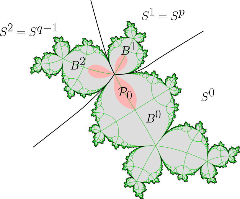
P\mathrm{P} has a parabolic fixed point at 0 with eigenvalue ω\omega and a critical point at −ω/2-\omega/2, with critical value −ω2/4-\omega^{2}/4. Let AA denote the parabolic basin of 0. The parabolic basin AA has a qq-cycle of components, whose closures meet only at the parabolic fixed point 0. These qq components perform a p/qp/q rotation around the fixed point 0, under iteration by P\mathrm{P}. They will be indexed counterclockwise with respect to their cyclic ordering B0,…,Bq−1B^{0},...,B^{q-1}, where B0B^{0} is the component that contains the critical point −ω/2-\omega/2. See Figure 1.

Let ϕ:A→ℂ\phi:A\to\mathbb{C} denote an extended Fatou coordinate, which is a surjective and holomorphic map that satisfies the Abel functional equation ϕ∘Pq=1+ϕ\phi\circ\mathrm{P}^{q}=1+\phi. It is patched together between components BjB^{j} to satisfy the functional equation:

ϕ∘P=1/q+ϕ.\phi\circ\mathrm{P}=1/q+\phi. (2)

The Fatou coordinate will be further normalized by setting ϕ(−ω/2)=0\phi(-\omega/2)=0.

Each BjB^{j} contains a unique petal 𝒫Δj⊆Bj\mathcal{P}_{\Delta}^{j}\subseteq B^{j} for Pq\mathrm{P}^{q} at 0, which is mapped univalently by ϕ\phi onto some right half-plane ℍΔ={z∈ℂ|ℜ⁡(z)>Δ}\mathbb{H}_{\Delta}=\{z\in\mathbb{C}\>|\>\Re(z)>\Delta\} and which is maximal in this sense, whence it has a critical point of Pq\mathrm{P}^{q} on its boundary. Such a petal is called a maximal attracting petal. In general, denote by 𝒫δj⊆Bj\mathcal{P}_{\delta}^{j}\subseteq B^{j} an attracting petal for Pq\mathrm{P}^{q} at 0, whose (univalent) image under ϕ\phi is precisely the right half-plane ℍδ={z∈ℂ|ℜ⁡(z)>δ}\mathbb{H}_{\delta}=\{z\in\mathbb{C}\>|\>\Re(z)>\delta\}. Note that by our choice of normalization 𝒫Δ0=𝒫00\mathcal{P}_{\Delta}^{0}=\mathcal{P}_{0}^{0}. We will say that a petal 𝒫δj\mathcal{P}_{\delta}^{j} is of level δ\delta and call the union 𝒫δ=⋃j∈ℤq𝒫δj\mathcal{P}_{\delta}=\bigcup_{j\in\mathbb{Z}_{q}}\mathcal{P}_{\delta}^{j} an attracting flower for P\mathrm{P} at 0 of level δ\delta. Let 𝒫^δ=𝒫δ∪{0}\widehat{\mathcal{P}}_{\delta}=\mathcal{P}_{\delta}\cup\{0\}.

The set A¯∖{0}\overline{A}\setminus\{0\} has qq connected components. Let SjS^{j} denote the component so that Bj⊂SjB^{j}\subset S^{j}, whence S0S^{0} is the component containing the critical point −ω/2-\omega/2 and SpS^{p} the component containing the critical value −ω2/4-\omega^{2}/4.

Refer to caption Refer to caption
Figure 1: The left picture shows AA, the attracting basin of 0, for P=P1/3\mathrm{P}=\mathrm{P}_{1/3}. The attracting flower 𝒫0\mathcal{P}_{0} is shown in pink. The figure also illustrates components BjB^{j} and sectors SjS^{j}. The right picture shows 𝒜m∗\mathcal{A}_{m}^{*}, with the removed sepals shown in dark grey, and the removed (extended) flower 𝒫^1/q\widehat{\mathcal{P}}_{1/q} shown in pink. Dynamical pictures are made by Arnaud Chéritat.

Let

𝒜=A∪⋃n≥0P−n​(0)⊂A¯,\mathcal{A}=A\cup\bigcup_{n\geq 0}\mathrm{P}^{-n}(0)\subset\overline{A}, (3)

and for m>0m>0 let

𝒜m=𝒜⁡(m)={z∈A:|ℑ⁡(ϕ⁡(z))|<m/2}∪⋃n≥0P−n​(0)⊂𝒜.\mathcal{A}_{m}=\mathcal{A}(m)=\left\{z\in A:|\Im(\phi(z))|<m/2\right\}\cup\bigcup_{n\geq 0}\mathrm{P}^{-n}(0)\subset\mathcal{A}. (4)

We will also allow m=∞m=\infty, in which case 𝒜m=𝒜\mathcal{A}_{m}=\mathcal{A}. The set 𝒜\mathcal{A} is the parabolic basin, augmented with 0 and all its pre-images, and 𝒜m\mathcal{A}_{m} has all so-called sepals of height m/2m/2, and all their pre-images, removed.

Recall that 𝒫1/q\mathcal{P}_{1/q} denotes the attracting flower for P\mathrm{P} at 0 of level 1/q1/q, and let

𝒜∗=𝒜∖(𝒫^1/q∪{−ω2/4})and\mathcal{A}^{*}=\mathcal{A}\setminus(\widehat{\mathcal{P}}_{1/q}\cup\{-\omega^{2}/4\})\quad\text{and} (5)
𝒜m∗=𝒜m∖(𝒫^1/q∪{−ω2/4}).\mathcal{A}^{*}_{m}=\mathcal{A}_{m}\setminus(\widehat{\mathcal{P}}_{1/q}\cup\{-\omega^{2}/4\}). (6)

See Figure 1. We are now ready to define dynamical marking relative to P\mathrm{P}.

2.1 Dynamical marking relative to P\mathrm{P}

For x∈𝒜∗x\in\mathcal{A}^{*}, let m>0m>0 be such that x∈𝒜m∗x\in\mathcal{A}_{m}^{*} and define

𝒰=𝒰m​(x):=P−n​(𝒫^0)∩𝒜m,\mathcal{U}=\mathcal{U}_{m}(x):=\mathrm{P}^{-n}(\widehat{\mathcal{P}}_{0})\cap\mathcal{A}_{m},

for n=n⁡(x)≥0n=n(x)\geq 0 minimal so that Pn​(x)∈𝒫^0\mathrm{P}^{n}(x)\in\widehat{\mathcal{P}}_{0}.

Note that 𝒰m​(x)\mathcal{U}_{m}(x) is forward invariant and connected, but neither open nor closed, and 0,−ω24,x∈𝒰m​(x)0,\frac{-\omega^{2}}{4},x\in\mathcal{U}_{m}(x), while P−1​(x)∩𝒰m​(x)=∅\mathrm{P}^{-1}(x)\cap\mathcal{U}_{m}(x)=\emptyset. To alleviate the notation, we use 𝒰=𝒰m​(x)\mathcal{U}=\mathcal{U}_{m}(x) if both xx and mm are clear from the context.

We define slit planes ℂ−ω=ℂ∖{−ω⋅r|r≥0}\mathbb{C}_{-\omega}=\mathbb{C}\setminus\{-\omega\cdot r\;|\;r\geq 0\} and disks 𝔻−ω=𝔻∖[0,−ω)\mathbb{D}_{-\omega}=\mathbb{D}\setminus[0,-\omega). For λ∈𝔻−ω\lambda\in\mathbb{D}_{-\omega} let L=q​Log⁡(λ​ω¯)=q​log⁡λ−p​2​π​iL=q{\operatorname{Log}}(\lambda\bar{\omega})=q\log\lambda-p2\pi i, where Log{\operatorname{Log}} is the principal logarithm, whence log\log is the branch of the logarithm from the cut plane ℂ−ω\mathbb{C}_{-\omega} to the strip {z∈ℂ| 2​π​p/q−π<ℑ⁡(z)<2​π​p/q+π}\{z\in\mathbb{C}\,|\;2\pi p/q-\pi<\Im(z)<2\pi p/q+\pi\}. For λ∈𝔻−ω∪{ω}\lambda\in\mathbb{D}_{-\omega}\cup\{\omega\} let

m⁡(λ)={2​π​sin⁡θq​|L| for ​λ≠ω∞ for ​λ=ω,m(\lambda)=\begin{cases}\frac{2\pi\sin\theta}{q|L|}&\text{ for }\lambda\neq\omega\\ \infty&\text{ for }\lambda=\omega,\end{cases} (7)

where θ\theta is the angle between LL and 2​π​i2\pi i. For λ≠ω\lambda\neq\omega the number rλ=πq2​m​(λ)r_{\lambda}=\frac{\pi}{q^{2}m(\lambda)} is the radius of the circle through log⁡λ\log\lambda, and tangent to the imaginary axis at 2​π​i​p/q2\pi ip/q, see also Section 4.

Definition 1 (Dynamical marking relative to P\mathrm{P}).

Let λ∈𝔻−ω∪{ω}\lambda\in\mathbb{D}_{-\omega}\cup\{\omega\} and m=m⁡(λ)m=m(\lambda), let σ∈ℛλ\sigma\in\mathcal{R}^{\lambda} and let g∈Γλ,σg\in\Gamma_{\lambda,\sigma} with a fixed point at z0z_{0} of eigenvalue λ\lambda. A dynamical marking of gg relative to P\mathrm{P} (written rel P\mathrm{P}) is a pair (x,ψ)(x,\psi) where x∈𝒜m⁡(λ)∗x\in\mathcal{A}^{*}_{m(\lambda)} and ψ:𝒰→V\psi:\mathcal{U}\to V is a homeomorphism obeying

ψ∘P=g∘ψ,\psi\circ\mathrm{P}=g\circ\psi, (8)

which is holomorphic on int⁡(𝒰)\operatorname{int}(\mathcal{U}), where ψ⁡(−ω24)\psi(-\frac{\omega^{2}}{4}) and ψ⁡(x)\psi(x) are the critical values of gg, and where 𝒰=𝒰m⁡(λ)​(x)\mathcal{U}=\mathcal{U}_{m(\lambda)}(x) as defined above.

Refer to caption
Figure 2: Illustrates dynamical marking rel P\mathrm{P} for p/q=1/3p/q=1/3. The left shows the dynamical plane of a g∈Γω1/3,σg\in\Gamma_{\omega_{1/3},\sigma} (on the Riemann sphere), and the filled-in Julia set of P\mathrm{P} is on the right. The figure shows the domain 𝒰⁡(x)\mathcal{U}(x) and range VV of ψ\psi in pink, the marking x∈𝒜∗x\in\mathcal{A}^{*} of gg and the two critical values v1v_{1} and v2v_{2} of gg. Dynamical pictures are made by Arnaud Chéritat.

When P\mathrm{P} is understood from the context, we will omit ”rel P\mathrm{P}”. We will say that gg is dynamically marked by (x,ψ)(x,\psi) if (x,ψ)(x,\psi) is a dynamical marking of gg. We will say that gg is dynamically marked by xx, if there exists a marker map ψ\psi, so that gg is dynamically marked by (x,ψ)(x,\psi). A dynamical marking induces a labeling v1=ψ⁡(−ω24)v_{1}=\psi(-\frac{\omega^{2}}{4}) and v2=ψ⁡(x)v_{2}=\psi(x) of critical values of gg. We will refer to this labeling as a dynamical labeling of gg.

For λ∈𝔻−ω∪{ω}\lambda\in\mathbb{D}_{-\omega}\cup\{\omega\} and σ∈ℛλ\sigma\in\mathcal{R}^{\lambda}, if g∈Γλ,σg\in\Gamma_{\lambda,\sigma} is dynamically marked by (x,ψ)(x,\psi) rel P\mathrm{P}, then xx is a conformal invariant of Γλ,σ\Gamma_{\lambda,\sigma}. Moreover, we will show that σ\sigma is the unique parameter in ℛλ\mathcal{R}^{\lambda}, which is dynamically marked by xx, and that the dynamical marker map ψ\psi is unique up to automorphisms of gg, see Proposition 1 (and its proof in Section 5.2) and Proposition 7 in Section 5.3. In view of these properties, we will speak of xx as a dynamical marking of the equivalence class Γλ,σ\Gamma_{\lambda,\sigma}, or of its parameter σ∈ℛλ\sigma\in\mathcal{R}^{\lambda}.

2.2 Parametrization of ℛ\mathcal{R} by dynamical marking rel P\mathrm{P}

Consider an M>1/q2M>1/q^{2} and let

DM={λ∈𝔻−ω:m⁡(λ)>M}.D_{M}=\{\lambda\in\mathbb{D}_{-\omega}:m(\lambda)>M\}.

DMD_{M} is the 𝔻∗\mathbb{D}^{*} horodisk exp⁡(𝔻⁡(−r+2​π​i​p/q,r))\exp(\mathbb{D}(-r+2\pi ip/q,r)) at ω\omega, where r=πq2​M<πr=\frac{\pi}{q^{2}M}<\pi, see Figure 3.

Figure 3: The figure illustrates 𝔻⁡(−r+2​π​i​p/q,r)\mathbb{D}(-r+2\pi ip/q,r), DMD_{M} and ρx\rho_{x} for p/q=1/3p/q=1/3 and M=1/3M=1/3.

Suppose λ∈𝔻−ω\lambda\in\mathbb{D}_{-\omega} is given. If xx is a dynamical marking of a σ∈ℛλ\sigma\in\mathcal{R}^{\lambda}, then xx is necessarily in 𝒜m⁡(λ)∗\mathcal{A}_{m(\lambda)}^{*}, thus 𝒜m⁡(λ)∗\mathcal{A}_{m(\lambda)}^{*} is the set of admissible xx-values for λ\lambda. On the other hand, suppose x∈𝒜∗x\in\mathcal{A}^{*} is fixed and let M>max⁡{1/q2,2​|ℑ⁡(ϕ⁡(x))|}M>\max\{1/q^{2},2|\Im(\phi(x))|\}, where it is understood (whenever it appears) that the maximum is equal to 1q2\frac{1}{q^{2}} when xx is not in the domain of ϕ\phi. Then x∈𝒜M∗x\in\mathcal{A}_{M}^{*} and the corresponding horodisk DMD_{M} consists of admissible values of λ\lambda. Fixing an MM determines a domain DM×𝒜M∗D_{M}\times\mathcal{A}_{M}^{*} of admissible pairs (λ,x)(\lambda,x) for dynamical markings in ℛ\mathcal{R}, since (λ,x)∈DM×𝒜M∗⇒x∈𝒜M∗⊂𝒜m⁡(λ)∗(\lambda,x)\in D_{M}\times\mathcal{A}_{M}^{*}\Rightarrow x\in\mathcal{A}^{*}_{M}\subset\mathcal{A}_{m(\lambda)}^{*}.

Not every σ∈ℛλ\sigma\in\mathcal{R}^{\lambda} is dynamically marked relative to P\mathrm{P} (see Section 5.2), but every x∈𝒜M∗x\in\mathcal{A}_{M}^{*} is the dynamical marking of exactly one σ∈ℛλ\sigma\in\mathcal{R}^{\lambda}, for each λ∈DM\lambda\in D_{M}.

Proposition 1.

Suppose M>1/q2M>1/q^{2}. For any (λ,x)∈DM×𝒜M∗(\lambda,x)\in D_{M}\times\mathcal{A}_{M}^{*}, there exists a unique parameter σ∈ℛλ\sigma\in\mathcal{R}^{\lambda} such that Γλ,σ\Gamma_{\lambda,\sigma} is dynamically marked by xx rel P\mathrm{P}. In particular, this defines a partial parametrization by dynamical marking, Φλ:𝒜M∗→ℛλ\Phi^{\lambda}:\mathcal{A}^{*}_{M}\to\mathcal{R}^{\lambda}. The map Φλ\Phi^{\lambda} is holomorphic in the interior of its domain, continuous when restricted to P−n​(𝒫^0)∩𝒜M∗\mathrm{P}^{-n}(\widehat{\mathcal{P}}_{0})\cap\mathcal{A}^{*}_{M} for every nn, but not in the entire domain 𝒜M∗\mathcal{A}^{*}_{M}, and depends analytically on the parameter λ∈DM\lambda\in D_{M}.

Moreover, if

  • •

    x∉∂𝒫1/qx\notin\partial\mathcal{P}_{1/q} then xx is the unique marking of Γλ,σ\Gamma_{\lambda,\sigma}.

  • •

    if x∈∂𝒫1/qp+jx\in\partial\mathcal{P}_{1/q}^{p+j} then x′∈∂𝒫1/qp−jx^{\prime}\in\partial\mathcal{P}_{1/q}^{p-j} with ℑ⁡(ϕ⁡(x′))=−ℑ⁡(ϕ⁡(x))\Im(\phi(x^{\prime}))=-\Im(\phi(x)), both p+jp+j and p−jp-j taken modulo qq, is the only other marking of Γλ,σ\Gamma_{\lambda,\sigma}.

The proposition will be proved in Section 5.2. We will use this result to define a partial parameter 𝚽\mathbf{\Phi} on ℛ\mathcal{R}, which parametrizes by dynamical marking relative to P\mathrm{P}.

Definition 2 (Definition of a partial parameter 𝚽\mathbf{\Phi} on ℛ\mathcal{R}).

For every p/q{p/q}, with (p,q)=1(p,q)=1 and q≥2q\geq 2, and for M>1q2M>\frac{1}{q^{2}} we define a map

𝚽:DM×𝒜M∗→(DM×ℂ)∩ℛof the form\mathbf{\Phi}:D_{M}\times\mathcal{A}_{M}^{*}\to(D_{M}\times\mathbb{C})\cap\mathcal{R}\quad\text{of the form}
𝚽⁡(λ,x)=(λ,Φ⁡(λ,x))=(λ,Φλ​(x))=(λ,Φx​(λ)),\mathbf{\Phi}(\lambda,x)=(\lambda,\Phi(\lambda,x))=(\lambda,\Phi^{\lambda}(x))=(\lambda,\Phi_{x}(\lambda)),

by letting Φλ:𝒜M∗→ℛλ\Phi^{\lambda}:\mathcal{A}^{*}_{M}\to\mathcal{R}^{\lambda} be the parametrization from Proposition 1. That is, Φλ​(x)=σ\Phi^{\lambda}(x)=\sigma, where σ\sigma is the unique parameter in ℛλ\mathcal{R}^{\lambda} so that Γλ,σ\Gamma_{\lambda,\sigma} is dynamically marked by xx rel P\mathrm{P}.

From Proposition 1 it follows that Φx\Phi_{x} is analytic in DMD_{M} for every x∈𝒜M∗x\in\mathcal{A}^{*}_{M}, we say that 𝚽\mathbf{\Phi} is horizontally analytic. For a fixed x∈𝒜M∗x\in\mathcal{A}^{*}_{M}, and for a curve δ⊂DM\delta\subset D_{M} or a sequence (λk)k⊂DM(\lambda_{k})_{k}\subset D_{M}, we will call Φx​(δ)\Phi_{x}(\delta) an xx-horizontal curve and (Φx​(λk))k(\Phi_{x}(\lambda_{k}))_{k} an xx-horizontal sequence. Every parameter in such an xx-horizontal curve or sequence has dynamical marking xx. For any x∈𝒜∗x\in\mathcal{A}^{*} if we let M>max⁡{1/q2,2​|ℑ⁡(ϕ⁡(x))|}M>\max\{1/q^{2},2|\Im(\phi(x))|\} then x∈𝒜M∗x\in\mathcal{A}_{M}^{*}. Thus, every x∈𝒜∗x\in\mathcal{A}^{*} and every sequence (λk)k⊂DM(\lambda_{k})_{k}\subset D_{M} give rise to sequences (λk,σk)=(λk,Φx​(λk))∈DM×ℂ(\lambda_{k},\sigma_{k})=(\lambda_{k},\Phi_{x}(\lambda_{k}))\in D_{M}\times\mathbb{C}, where each σk∈ℛλk\sigma_{k}\in\mathcal{R}^{\lambda_{k}} and (σk)k(\sigma_{k})_{k} is an xx-horizontal sequence.

Main result 1: Convergence to the parabolic locus ℛω\mathcal{R}^{\omega}

The following Theorem is a main result of this paper. It is concerned with the limiting behavior of such xx-horizontal sequences (λk,σk)(\lambda_{k},\sigma_{k}) in ℛ⊂ℂ2\mathcal{R}\subset\mathbb{C}^{2} as λk→ω\lambda_{k}\to\omega subhorocyclicly.

Theorem 1.

For x∈𝒜∗∖Spx\in\mathcal{A}^{*}\setminus S^{p}, let M>max⁡{1/q2,2​|ℑ⁡(ϕ⁡(x))|}M>\max\{1/q^{2},2|\Im(\phi(x))|\} and let (λk)k⊂DM(\lambda_{k})_{k}\subset D_{M} be a sequence converging to ω=ωp/q\omega=\omega_{p/q} subhorocyclicly. Then the xx-horizontal sequence (σk)k=(Φx​(λk))k(\sigma_{k})_{k}=(\Phi_{x}(\lambda_{k}))_{k} converges to the unique σ∈ℛω∖𝒟ω\sigma\in\mathcal{R}^{\omega}\setminus\mathcal{D}^{\omega}, which is dynamically marked by xx rel P\mathrm{P}. In particular, every x∈𝒜∗∖Spx\in\mathcal{A}^{*}\setminus S^{p} is a dynamical marking for exactly one σ∈ℛω∖𝒟ω\sigma\in\mathcal{R}^{\omega}\setminus\mathcal{D}^{\omega}.

In the other direction, dynamical marker maps for parameters σ∈ℛω∖𝒟ω\sigma\in\mathcal{R}^{\omega}\setminus\mathcal{D}^{\omega} can be constructed using Fatou coordinates. This is done in [U] (although it is not called dynamical markings). [U, Lemma 3.3] shows that no σ∈ℛω∖𝒟ω\sigma\in\mathcal{R}^{\omega}\setminus\mathcal{D}^{\omega} is dynamically marked, rel P\mathrm{P}, by an x∈Spx\in S^{p}. For completeness, the next proposition formulates the results from [U] in the context of dynamical markings, and we recall the construction of dynamical marker maps for g∈Γω,σg\in\Gamma_{\omega,\sigma} with σ∈ℛω∖𝒟ω\sigma\in\mathcal{R}^{\omega}\setminus\mathcal{D}^{\omega} in its proof in Section 5.3.

Proposition 2.

Any σ∈ℛω∖𝒟ω\sigma\in\mathcal{R}^{\omega}\setminus\mathcal{D}^{\omega} is dynamically marked rel P\mathrm{P} by an x∈𝒜∗∖Spx\in\mathcal{A}^{*}\setminus S^{p}. If x∉∂𝒫1/qx\notin\partial\mathcal{P}_{1/q} then xx is the unique marking of σ\sigma. On the other hand if x∈∂𝒫1/qp+jx\in\partial\mathcal{P}_{1/q}^{p+j} then x′∈∂𝒫1/qp−jx^{\prime}\in\partial\mathcal{P}_{1/q}^{p-j} with ℑ⁡(ϕ⁡(x′))=−ℑ⁡(ϕ⁡(x))\Im(\phi(x^{\prime}))=-\Im(\phi(x)), both p+jp+j and p−jp-j taken modulo qq, is the only other marking of σ\sigma.

Proposition 2 and Theorem 1 together show that dynamical marking rel P\mathrm{P} gives rise to a surjective and almost injective parameter from 𝒜∗∖Sp\mathcal{A}^{*}\setminus S^{p} onto ℛω∖𝒟ω\mathcal{R}^{\omega}\setminus\mathcal{D}^{\omega}, and they imply the following corollary.

For x∈𝒜∗∖Spx\in\mathcal{A}^{*}\setminus S^{p} let M=max⁡{1/q2,2​|ℑ⁡(ϕ⁡(x))|}M=\max\{1/q^{2},2|\Im(\phi(x))|\} and let

ρx=e−2​πq2​M,\rho_{x}=e^{\frac{-2\pi}{q^{2}M}},

it is the ”diameter” of the 𝔻∗\mathbb{D}^{*} horodisk DMD_{M}, see Figure 3.

Corollary 1.

Every σ∈ℛω∖𝒟ω\sigma\in\mathcal{R}^{\omega}\setminus\mathcal{D}^{\omega} is accessible from the Cantor locus ℛ\mathcal{R}. Let xx be a dynamical marking rel P\mathrm{P} of σ\sigma. Then the xx-horizontal analytic curve δx=(Φx:ω]ρx,1[→ℂ)\delta_{x}=(\Phi_{x}:\omega]\rho_{x},1[\to\mathbb{C}) lands at σ\sigma, that is δx\delta_{x} extends continuously to 1 with δx​(1)=σ\delta_{x}(1)=\sigma.

2.3 Main result 2: Divergence and rescaling

As described above, no σ∈ℛω∖𝒟ω\sigma\in\mathcal{R}^{\omega}\setminus\mathcal{D}^{\omega} is dynamically marked rel P\mathrm{P} by an x∈Spx\in S^{p}, so what happens for sequences (λk,σk=Φx​(λk))k(\lambda_{k},\sigma_{k}=\Phi_{x}(\lambda_{k}))_{k}, for x∈Spx\in S^{p}, as λk\lambda_{k} tends to ωp/q\omega_{p/q}? That is the topic of the next theorem, but first we need a little more background.

The definition of dynamical marking relative to Pω\mathrm{P}_{\omega} also makes sense for the case ω=1\omega=1. We let A1A_{1} denote the parabolic basin of 0 for P1\mathrm{P}_{1}, and let ϕ1\phi_{1} denote the extended Fatou coordinate, normalized so that ϕ1(−1/4)=1\phi_{1}(-1/4)=1. Petals 𝒫δ\mathcal{P}_{\delta} are defined in the same way as for q≥2q\geq 2, and we let

A~1=A1∪⋃n≥0P1−n​(0)\widetilde{A}_{1}=A_{1}\cup\bigcup_{n\geq 0}\mathrm{P}_{1}^{-n}(0) (9)

and

A1∗=A~1∖(𝒫1∪{0,−1/4}).A_{1}^{*}=\widetilde{A}_{1}\setminus(\mathcal{P}_{1}\cup\{0,-1/4\}). (10)

Dynamical markings x∈A1∗x\in A_{1}^{*}, the corresponding marker maps ψ\psi, and their domains are defined similarly to the case q≥2q\geq 2.

Recall that the set A¯∖{0}\overline{A}\setminus\{0\} (for P\mathrm{P}) has qq connected components and that S0S^{0} is the component containing the critical point −ω/2-\omega/2, see again Figure 1.

Refer to caption
Figure 4: The figure illustrates the map h1h_{1} (for p/q=1/3p/q=1/3), with the augmented basin 𝒜\mathcal{A} of P\mathrm{P} on the left and the augmented basin A~1\widetilde{A}_{1} of P1\mathrm{P}_{1} on the right (to the level n=2n=2 for A~1\widetilde{A}_{1}). h1h_{1} maps the sets C⁡(z0)C(z_{0}) to h1​(z0)h_{1}(z_{0}). The figure also illustrates h1​(Pq−1​(x))h_{1}(\mathrm{P}^{q-1}(x)), cf. Theorem 2. Dynamical pictures by Arnaud Chéritat.
Connecting Pq\mathrm{P}^{q} on S0¯∩𝒜\overline{S^{0}}\cap\mathcal{A} to P1\mathrm{P}_{1} on A~1\widetilde{A}_{1}

We introduce a surjective, continuous map h1:S0¯∩𝒜→A~1h_{1}:\overline{S^{0}}\cap\mathcal{A}\to\widetilde{A}_{1}, with h1​(0)=0h_{1}(0)=0 and h1(−ω/2)=−1/2h_{1}(-\omega/2)=-1/2, such that

h1∘Pq=P1∘h1on ​B0¯∩𝒜.h_{1}\circ\mathrm{P}^{q}=\mathrm{P}_{1}\circ h_{1}\quad\text{on }\overline{B^{0}}\cap\mathcal{A}. (11)

On B0B^{0} it is the biholomorphic conjugacy h1:B0→A~1h_{1}:B^{0}\to\widetilde{A}_{1} of Pq\mathrm{P}^{q} to P1\mathrm{P}_{1}, constructed from Fatou coordinates for Pq\mathrm{P}^{q} and P1\mathrm{P}_{1}, such that h1(−ω/2)=−1/2h_{1}(-\omega/2)=-1/2. It is extended to the fixed point 0 and all its pre-images by continuity, so that, in particular, h1​(0)=0h_{1}(0)=0. This defines h1h_{1} as a homeomorphic conjugacy from B0¯∩𝒜\overline{B^{0}}\cap\mathcal{A} onto A~1\widetilde{A}_{1}. The next step is to extend h1h_{1} to the full domain. Let z0z_{0} denote an iterated pre-image of 0 in B0¯\overline{B^{0}}, every such pre-image of 0 separates S0S^{0} into qq connected components, let C⁡(z0)C(z_{0}) denote the union of components not containing −ω/2-\omega/2, and define h1​(z)=h1​(z0)h_{1}(z)=h_{1}(z_{0}) for all z∈C⁡(z0)z\in C(z_{0}), see Figure 4. Thus, informally speaking, h1h_{1} ”collapses” everything attached to B0B^{0} at z0z_{0} to the image of z0z_{0}. With this extension h1h_{1} is continuous and surjective, but of course no longer a bijection, and it does not obey the functional equation (11) everywhere.

For ω=1\omega=1 we use the normal form GT​(z):=G1,T​(z)=z+T+1zG_{T}(z):=G_{1,T}(z)=z+T+\frac{1}{z}. The next Theorem is the analogue of Theorem 1 for x∈Spx\in S^{p}.

Theorem 2.

For every x∈𝒜∗∩Spx\in\mathcal{A}^{*}\cap S^{p} let M>max⁡{1/q2,2​|ℑ⁡(ϕ⁡(x))|}M>\max\{1/q^{2},2|\Im(\phi(x))|\} and let (λk)k⊂DM(\lambda_{k})_{k}\subset D_{M} be a sequence converging to ω=ωp/q\omega=\omega_{p/q} subhorocyclicly. Then the xx-horizontal sequence σk=Φx​(λk)\sigma_{k}=\Phi_{x}(\lambda_{k}) tends to ∞∈ℂ^\infty\in\widehat{\mathbb{C}}.

Moreover, for representatives Gλk,ak∈𝚪λk,σkG_{\lambda_{k},a_{k}}\in{{\mbox{\boldmath$\Gamma$}}}_{\lambda_{k},\sigma_{k}} with dynamical labeling ψk​(−λk24)=Gλk,ak​(1)\psi_{k}\left(-\frac{\lambda_{k}^{2}}{4}\right)=G_{\lambda_{k},a_{k}}(1) and ψk​(x)=Gλk,ak​(−1)\psi_{k}(x)=G_{\lambda_{k},a_{k}}(-1) rel P\mathrm{P}, it holds that

  • •

    Gλk,ak→∞G_{\lambda_{k},a_{k}}\to\infty locally uniformly on ℂ∗\mathbb{C}^{*}

  • •

    Gλk,akq→GTG_{\lambda_{k},a_{k}}^{q}\to G_{T} locally uniformly on ℂ∗\mathbb{C}^{*}, where T∈ℂT\in\mathbb{C}, σ=1−T2∈ℛ1\sigma=1-T^{2}\in\mathcal{R}^{1} and σ\sigma is dynamically marked by h1​(Pq−1​(x))h_{1}(\mathrm{P}^{q-1}(x)) rel P1\mathrm{P}_{1}.

    In particular, if x∈Bpx\in B^{p}, then both critical points ±1\pm 1 of GTG_{T} are in the same component of the parabolic basin of ∞\infty and σ∈int⁡(ℛ1)=ℂ∖M1\sigma\in\operatorname{int}(\mathcal{R}^{1})=\mathbb{C}\setminus M^{1}. And if x∈Sp∖Bpx\in S^{p}\setminus B^{p} then there exists n≥1n\geq 1 so that GTn​(−1)=0G^{n}_{T}(-1)=0 and σ∈ℛ1∩M1\sigma\in\mathcal{R}^{1}\cap M^{1}.

There are three main tools for the proofs. The first is the behavior of sequences that diverge to infinity in 𝐫𝐚𝐭2{\bf rat}_{2}, which is treated in [E]. We give a quick distillation of the results needed for our use in Section 3 and apply them to show new results concerning the Cantor locus in Section 6. The largely algebraic conditions in [E] are refined to our case in Lemma 9 (in Section 6), using the geometric control coming from the dynamical markings.

The second is a construction called stars in attracting basins, introduced in [P], and treated in Section 4. We define the construction in Section 4.1, and use it to introduce dynamical markings rel Pλ\mathrm{P}_{\lambda} (for λ∈𝔻−ω\lambda\in\mathbb{D}_{-\omega}) in Section 4.2. The third tool is a model for ℛλ\mathcal{R}^{\lambda}, which is modified from a model introduced in [GK]. Our formulation of the model is based on stars and dynamical markings, it is given in Section 4.3.

In Sections 4.4 and 4.5 we treat stars in non-simply connected quadratic basins; we show some new results and extend a main result from [P] to this case. In Section 5 we prove Proposition 1 and Proposition 2, and show uniqueness of dynamical markings rel P\mathrm{P}. The paper ends with the proofs of Theorems 1 and 2 in Section 6.

3 Divergence to infinity in 𝐫𝐚𝐭2{\bf rat}_{2}

3.1 Reminder on normal forms

For polynomials with an attracting or parabolic fixed point we use

Pλ​(z)=λ​z+z2,λ∈𝔻∗∪⋃p/q{ωp/q}.\mathrm{P}_{\lambda}(z)=\lambda z+z^{2},\quad\lambda\in\mathbb{D}^{*}\cup\bigcup_{p/q}\{\omega_{p/q}\}.

Pλ\mathrm{P}_{\lambda} has an attracting or parabolic fixed point at 0 with eigenvalue λ\lambda and a critical point at −λ2\frac{-\lambda}{2}, with critical value −λ24\frac{-\lambda^{2}}{4}.

Every quadratic rational map has three fixed points, counting multiplicity, and two critical points with distinct critical values. Recall that each class 𝚪λ,σ{{\mbox{\boldmath$\Gamma$}}}_{\lambda,\sigma} in Per1⁡(λ)\operatorname{Per}_{1}(\lambda) has a representative of the form

Gλ,a​(z)=1λ​(z+a+1z),G_{\lambda,a}(z)=\frac{1}{\lambda}\left(z+a+\frac{1}{z}\right), (12)

as long as λ≠0\lambda\neq 0. Maps Gλ,aG_{\lambda,a} have critical points ±1\pm 1 and a fixed point at ∞\infty with eigenvalue λ\lambda. Note that [Gλ,a]=[Gλ,−a]=𝚪λ,σ[G_{\lambda,a}]=[G_{\lambda,-a}]={{\mbox{\boldmath$\Gamma$}}}_{\lambda,\sigma} where

σ=(λ−2)2−a2λ2.\sigma=\frac{(\lambda-2)^{2}-a^{2}}{\lambda^{2}}. (13)

For the case λ=1\lambda=1 we use the notation:

GT​(z):=G1,T​(z)=z+T+1z,GT∈𝚪1,σ,G_{T}(z):=G_{1,T}(z)=z+T+\frac{1}{z},\quad G_{T}\in{{\mbox{\boldmath$\Gamma$}}}_{1,\sigma}, (14)

where σ=1−T2\sigma=1-T^{2}. Maps GTG_{T} have critical points ±1\pm 1 and a double fixed point at ∞\infty with eigenvalue 1.

3.2 Dynamics near infinity in 𝐫𝐚𝐭2{\bf rat}_{2}

The moduli space 𝐫𝐚𝐭2{\bf rat}_{2} contains infinitely many unbounded and infinitely many bounded components. Every hyperbolic component of maps with an attracting fixed point is unbounded. Epstein shows [E] that every hyperbolic component of maps with two distinct attracting cycles has compact closure in 𝐫𝐚𝐭2{\bf rat}_{2} if and only if neither attractor is a fixed point. One of the tools for this is a detailed understanding of those unbounded sequences in 𝐫𝐚𝐭2{\bf rat}_{2}, which have a fixed point eigenvalue tending to a qqth root of unity. [E] studies sequences of maps Gλk,ak​(z)=1λk​(z+ak+1z)G_{\lambda_{k},a_{k}}(z)=\frac{1}{\lambda_{k}}(z+a_{k}+\frac{1}{z}), so that λk\lambda_{k} tends to a qqth root of unity and [Gλk,ak][G_{\lambda_{k},a_{k}}] diverges to infinity in 𝐫𝐚𝐭2{\bf rat}_{2}. In particular [E] gives algebraic conditions under which the sequence of qqth iterates of such a sequence converges locally uniformly on ℂ∗\mathbb{C}^{*} to a quadratic rational map. We refer to this as rescaling.

We summarize here some results from [E] and [M1] concerning the dynamical behavior of sequences that diverge to infinity in 𝐫𝐚𝐭2{\bf rat}_{2}. For the formulation of Lemma 1([E]) given here, see also [K] and [EU].

A sequence is bounded in 𝐫𝐚𝐭2{\bf rat}_{2} if and only if the corresponding sequences of the eigenvalues of the fixed points λk,μk,νk\lambda_{k},\mu_{k},\nu_{k} are bounded in ℂ\mathbb{C}. The well-known holomorphic index formula, which for λ,μ≠1\lambda,\mu\neq 1 can be written as

ν=2−λ−μ1−λ​μ,\nu=\frac{2-\lambda-\mu}{1-\lambda\mu},

shows that if λk,μk\lambda_{k},\mu_{k} tend to λ,1λ\lambda,\frac{1}{\lambda}, for some λ∈ℂ^∖{1}\lambda\in\widehat{\mathbb{C}}\setminus\{1\}, then σk=μk​νk→∞\sigma_{k}=\mu_{k}\nu_{k}\to\infty.

For the other direction, any unbounded sequence in 𝐫𝐚𝐭2{\bf rat}_{2} has a subsequence, such that the fixed point eigenvalues tend to λ,1λ,∞\lambda,\frac{1}{\lambda},\infty, where λ∈ℂ^\lambda\in\widehat{\mathbb{C}}. Here we consider sequences 𝚪λk,σk{{\mbox{\boldmath$\Gamma$}}}_{\lambda_{k},\sigma_{k}} where λk→ωp/q\lambda_{k}\to\omega_{p/q}.

Lemma 1 ([E]).

Let fkf_{k} be a sequence of quadratic rational maps, with fixed point eigenvalues λk,μk,νk\lambda_{k},\mu_{k},\nu_{k} tending to ωp/q,ω¯p/q,∞\omega_{p/q},\bar{\omega}_{{p/q}},\infty, q≥2q\geq 2. If fk=Gλk,akf_{k}=G_{\lambda_{k},a_{k}} then

fki→∞ locally uniformly on ​ℂ∗​ for ​1≤i<q.f_{k}^{i}\to\infty\quad\text{ locally uniformly on }\mathbb{C}^{*}\text{ for }1\leq i<q.

If further 1−λkq1−λk⋅ak→T∈ℂ^\frac{1-\lambda_{k}^{q}}{1-\lambda_{k}}\cdot a_{k}\to T\in\widehat{\mathbb{C}}, then

fkq→GT locally uniformly on ​ℂ∗,f_{k}^{q}\to G_{T}\quad\text{ locally uniformly on }\mathbb{C}^{*},

where we use the convention G∞=∞G_{\infty}=\infty. Moreover, if T∈ℂT\in\mathbb{C}, λk≠ωp/q\lambda_{k}\neq\omega_{p/q} and μk≠ω¯p/q\mu_{k}\neq\bar{\omega}_{{p/q}} then there are qq-cycles ⟨z⟩k\langle z\rangle_{k} with eigenvalues ρk→1−T2\rho_{k}\to 1-T^{2}, while for any other qq-cycles ⟨z^⟩k≠⟨z⟩k\langle\widehat{z}\rangle_{k}\neq\langle z\rangle_{k} the eigenvalues tend to infinity.

4 Quadratic attracting basins

In this section we study quadratic rational maps belonging to the Cantor locus, that is, maps g∈𝚪λ,σg\in{{\mbox{\boldmath$\Gamma$}}}_{\lambda,\sigma} with λ∈𝔻∗\lambda\in\mathbb{D}^{*} and σ∈ℛλ\sigma\in\mathcal{R}^{\lambda}. As a tool for this, we introduce the concept of stars for attracting basins, in Section 4.1. The stars are used both for the definition of the parametrization 𝚽\mathbf{\Phi} from definition 2 and to classify the (un)boundedness of the sequences σk=Φλk​(x)\sigma_{k}=\Phi^{\lambda_{k}}(x) of Theorem 1 and 2. In order to construct the (partial) parametrization Φλ\Phi^{\lambda} of ℛλ\mathcal{R}^{\lambda} we introduce dynamical markings relative to Pλ\mathrm{P}_{\lambda} (Section 4.2 and Definition 4), and use them both as a model for the dynamics of maps g∈𝚪λ,σg\in{{\mbox{\boldmath$\Gamma$}}}_{\lambda,\sigma}, as well as to construct a model of the locus ℛλ\mathcal{R}^{\lambda} (see Proposition 3 and Section 4.3). The classification of the boundedness behavior of sequences σk=Φλk​(x)\sigma_{k}=\Phi^{\lambda_{k}}(x) is built on Yoccoz-type inequalities for certain eigenvalues, which are derived from modulus estimates from the star; see Sections 4.5 and 4.4, Proposition 5 and Corollary 2 and 3.

Stars for attracting basins were introduced by Petersen in [P], where the case of simply connected quadratic basins is studied. Our objective is infinitely connected quadratic basins. We will give an overview of the construction and properties of stars in the quadratic case, tailored to our application, and refer to [P] for more background. We extend main results from [P] to the case of infinitely connected basins of quadratic rational maps.

Given an irreducible rational number p/qp/q, (p,q)=1(p,q)=1, we define as before for λ∈ℂ∗∖𝕊1\lambda\in\mathbb{C}^{*}\setminus\mathbb{S}^{1} the vector L=L(p/q)=qLog(λe−i2πp/q)=qlogλ−p2πiL=L(p/q)=q{\operatorname{Log}}(\lambda{\operatorname{e}}^{-i2\pi p/q})=q\log\lambda-p2\pi i; here Log:ℂ∖(−∞,0]→ℂ{\operatorname{Log}}:{\mathbb{C}\setminus(-\infty,0]}\to\mathbb{C} is the principal branch of log\log and log⁡λ\log\lambda is an appropriate choice of logarithm of λ\lambda, see also Section 2, before Definition 1. We define also the number

rλ=rλ,p/q:=|L|2​q​sin⁡θ=πq2​m​(λ),r_{\lambda}=r_{\lambda,p/q}:=\frac{|L|}{2q\sin\theta}=\frac{\pi}{q^{2}m(\lambda)}, (15)

where θ\theta is the angle between LL and 2​π​i2\pi i and m⁡(λ)m(\lambda) is defined in Equation (7). The number rλr_{\lambda} is the radius of the circle through log⁡λ\log\lambda, and tangent to the imaginary axis at 2​π​i​p/q2\pi ip/q, see Figure 5.

Figure 5: The figure illustrates rλr_{\lambda}, log⁡λ\log\lambda, LL and θ\theta.

We now restrict our attention to λ∈𝔻−ω\lambda\in\mathbb{D}_{-\omega}. For λ∈𝔻−ω\lambda\in\mathbb{D}_{-\omega} and σ∈ℂ\sigma\in\mathbb{C}, let gλ,σ:ℂ^→ℂ^g_{\lambda,\sigma}:\widehat{\mathbb{C}}\to\widehat{\mathbb{C}} denote a quadratic rational map in 𝚪λ,σ{{\mbox{\boldmath$\Gamma$}}}_{\lambda,\sigma}, with the attracting fixed point of eigenvalue λ\lambda at z0z_{0}, so that gλ,σ​(z0)=z0g_{\lambda,\sigma}(z_{0})=z_{0} and gλ,σ′​(z0)=λg_{\lambda,\sigma}^{\prime}(z_{0})=\lambda. Let Aλ,σA_{\lambda,\sigma} denote the attracting basin of z0z_{0}. Such a map has an extended linearizing coordinate ϕλ,σ:Aλ,σ→ℂ\phi_{\lambda,\sigma}:A_{\lambda,\sigma}\to\mathbb{C}, which is a holomorphic and surjective map so that ϕλ,σ​(z0)=0\phi_{\lambda,\sigma}(z_{0})=0 and ϕλ,σ∘gλ,σ=λ⋅ϕλ,σ\phi_{\lambda,\sigma}\circ g_{\lambda,\sigma}=\lambda\cdot\phi_{\lambda,\sigma}. The linearizing coordinate is univalent on some neighborhood of the fixed point and unique up to multiplication by a non-zero constant. In our notation gλ,σg_{\lambda,\sigma} denotes a general quadratic rational map and could be a polynomial (σ=0\sigma=0). When we need to emphasize that the map in question is a polynomial, we use the notation introduced in Section 3 and choose the specific representative Pλ\mathrm{P}_{\lambda}.

In the following p/qp/q is fixed and LL is fixed for a given λ∈𝔻−ω\lambda\in\mathbb{D}_{-\omega}.

4.1 Definition of the (log⁡λ,p/q)(\log\lambda,p/q)-star of Aλ,σA_{\lambda,\sigma} for gλ,σg_{\lambda,\sigma}

The meromorphic vector field v⁡(z)​dd​zv(z)\frac{d}{dz}, given by v⁡(z)=L​ϕλ,σ​(z)ϕλ,σ′​(z)v(z)=L\frac{\phi_{\lambda,\sigma}(z)}{\phi_{\lambda,\sigma}^{\prime}(z)}, is independent of the choice of normalization of the linearizing coordinate ϕλ,σ\phi_{\lambda,\sigma} for gλ,σg_{\lambda,\sigma}. The flowlines of the vector field can be thought of as a singular foliation ℱ\mathcal{F} in Aλ,σ∖⋃n≥0gλ,σ−n​(z0)A_{\lambda,\sigma}\setminus\bigcup_{n\geq 0}g_{\lambda,\sigma}^{-n}(z_{0}). The following description is convenient to have in mind. The collection of lines parallel with LL, {ℝ​L+i​y:y∈ℝ}\{\mathbb{R}L+iy:y\in\mathbb{R}\} defines a foliation of ℂ\mathbb{C}, and the collection of logarithmic spirals {exp⁡(ℝ​L+i​y):y∈ℝ}\{\exp(\mathbb{R}L+iy):y\in\mathbb{R}\} defines a foliation of ℂ∗\mathbb{C}^{*}, with leaves exp⁡(ℝ​L+i​y)\exp(\mathbb{R}L+iy) emanating from infinity and ending at 0. The foliation ℱ\mathcal{F} in Aλ,σ∖⋃n≥0gλ,σ−n​(z0)A_{\lambda,\sigma}\setminus\bigcup_{n\geq 0}g_{\lambda,\sigma}^{-n}(z_{0}) is thus equivalently defined as the pullback of the foliation {exp⁡(ℝ​L+i​y):y∈ℝ}\{\exp(\mathbb{R}L+iy):y\in\mathbb{R}\} in ℂ∗\mathbb{C}^{*} by a linearizing coordinate ϕλ,σ\phi_{\lambda,\sigma}. See Figure 6.

Charts for ℱ\mathcal{F} (and linearizing coordinates for the vector field) are of the form log∘ϕλ,σL\frac{\log\circ\phi_{\lambda,\sigma}}{L}, where log\log is some branch of the logarithm and ϕλ,σ\phi_{\lambda,\sigma} as always a linearizing coordinate, whence changes of charts are translations. In this way, a choice of LL defines a unique holomorphic, singular foliation by curves in Aλ,σ∖⋃n≥0gλ,σ−n​(z0)A_{\lambda,\sigma}\setminus\bigcup_{n\geq 0}g_{\lambda,\sigma}^{-n}(z_{0}), with singular points precisely at the critical points of gλ,σg_{\lambda,\sigma} in Aλ,σ∖⋃n≥0gλ,σ−n​(z0)A_{\lambda,\sigma}\setminus\bigcup_{n\geq 0}g_{\lambda,\sigma}^{-n}(z_{0}) and their iterated pre-images.

Refer to caption
Figure 6: An illustration of leaves of the foliations in Aλ∖⋃n≥0Pλ−n​(0)A_{\lambda}\setminus\bigcup_{n\geq 0}\mathrm{P}_{\lambda}^{-n}(0), ℂ∗\mathbb{C}^{*} and ℂ\mathbb{C}, for p/q=1/3p/q=1/3 and λ=r​ω1/3\lambda=r\omega_{1/3} for an r>0r>0.

Leaves of ℱ\mathcal{F} either end (in infinite time) at z0z_{0} or one of its iterated pre-images, or connect two singular points of ℱ\mathcal{F}. A leaf whose closure contains z0z_{0} will be called a visible leaf. A visible leaf either begins in finite time at a singular point of ℱ\mathcal{F}, or continues in infinite time, both forward and backward. We will say that a point z∈Aλ,σz\in A_{\lambda,\sigma} is visible, if z=z0z=z_{0} or zz is in the interior of a visible leaf. For a visible point zz, the time-1 flow of the vector field is equal to the qqth iterate gλ,σq​(z)g_{\lambda,\sigma}^{q}(z), in particular, a visible leaf is forward invariant under gλ,σqg_{\lambda,\sigma}^{q}. Moreover, visible leaves are grouped in cycles of exact period qq, each performing a p/qp/q rotation under the map gλ,σg_{\lambda,\sigma}, as can be easily seen from the foliation of ℂ\mathbb{C} by {ℝ​L+i​y:y∈ℝ}\{\mathbb{R}L+iy:y\in\mathbb{R}\}.

There is always at least one visible critical value in Aλ,σ∖⋃n≥0gλ,σ−n​(z0)A_{\lambda,\sigma}\setminus\bigcup_{n\geq 0}g_{\lambda,\sigma}^{-n}(z_{0}), and in case σ∈ℛλ\sigma\in\mathcal{R}^{\lambda} there might be two. We will call a visible leaf a branch, if it begins at a singular point, every branch is part of a qq-cycle of branches containing a visible critical value. Let 1≤k′≤21\leq k^{\prime}\leq 2 denote the number of visible critical values of gλ,σg_{\lambda,\sigma}, let viv_{i}, 1≤i≤k′1\leq i\leq k^{\prime}, denote the visible critical values and cic_{i} the corresponding critical points. Let kk denote the number of cycles of branches, then 1≤k≤k′≤21\leq k\leq k^{\prime}\leq 2 with k<k′k<k^{\prime} if and only if k′=2k^{\prime}=2 and v1v_{1} and v2v_{2} belong to the same cycle of branches.

We name branches τij\tau_{i}^{j}, j∈ℤqj\in\mathbb{Z}_{q} and 1≤i≤k1\leq i\leq k, labelled counterclockwise with respect to their cyclic ordering, and so that cic_{i} is the start point of τi0\tau_{i}^{0} (when k′=2k^{\prime}=2 there is no preferred choice of ”first” visible critical value v1v_{1}).

We now elaborate on the description and properties of the leaves of the foliation. We choose a numbering of the critical values, by letting v1v_{1} denote (one of) the visible critical value(s). The linearizing coordinate is then normalized by setting ϕλ,σ​(v1)=λ\phi_{\lambda,\sigma}(v_{1})=\lambda, hence ϕλ,σ​(c1)=1\phi_{\lambda,\sigma}(c_{1})=1. Let ζi\zeta_{i} denote a logarithm of ϕλ,σ​(ci)\phi_{\lambda,\sigma}(c_{i}), where we normalize the logarithm by choosing ζ1\zeta_{1} to be 0.

Among the lines which are parallel to LL we give special attention to those giving rise to branches. Namely, let τ~ij\widetilde{\tau}_{i}^{j} denote the lines:

τ~ij:=t​L+jq​2​π​i+ζifor ​t∈ℝ,j∈ℤ​ and ​1≤i≤k,\widetilde{\tau}_{i}^{j}:=tL+\frac{j}{q}2\pi i+\zeta_{i}\quad\text{for }t\in\mathbb{R},j\in\mathbb{Z}\text{ and }1\leq i\leq k, (16)

and set

τ~i=⋃j∈ℤτ~ij and τ~=⋃1≤i≤kτ~i,\widetilde{\tau}_{i}=\bigcup_{j\in\mathbb{Z}}\widetilde{\tau}_{i}^{j}\quad\text{ and }\quad\widetilde{\tau}=\bigcup_{1\leq i\leq k}\widetilde{\tau}_{i},

where lines in τ~\widetilde{\tau} are named τ~j\widetilde{\tau}^{j} according to their horizontal ordering and so that τ~0=τ~10\widetilde{\tau}^{0}=\widetilde{\tau}_{1}^{0}. Note that when k=2k=2, τ~j≠τ~ij\widetilde{\tau}^{j}\neq\widetilde{\tau}_{i}^{j} in general, since each τ~1j\widetilde{\tau}_{1}^{j} is situated between τ~2j′\widetilde{\tau}_{2}^{j^{\prime}} and τ~2j′+1\widetilde{\tau}_{2}^{j^{\prime}+1} for some j′j^{\prime} and vice versa.

The collection of lines τ~\widetilde{\tau} bound open strips U~j\widetilde{U}^{j}, j∈ℤj\in\mathbb{Z}, which are named according to their horizontal ordering and so that U~0\widetilde{U}^{0} is bounded below by τ~0\widetilde{\tau}^{0}. Let γ~=⋃j∈ℤγ~j\widetilde{\gamma}=\bigcup_{j\in\mathbb{Z}}\widetilde{\gamma}^{j} denote the collection of central straight lines γ~j⊂U~j\widetilde{\gamma}^{j}\subset\widetilde{U}^{j}. Each line τ~ij\widetilde{\tau}_{i}^{j} and γ~j\widetilde{\gamma}^{j} and strip U~j\widetilde{U}^{j} is invariant under the translation z↦z+Lz\mapsto z+L, and each τ~ij\widetilde{\tau}_{i}^{j} is mapped to τ~ij+p\widetilde{\tau}_{i}^{j+p} (and τ~j\widetilde{\tau}^{j}, γ~j\widetilde{\gamma}^{j} and U~j\widetilde{U}^{j} to τ~j+k​p\widetilde{\tau}^{j+kp}, γ~j+k​p\widetilde{\gamma}^{j+kp} and U~j+k​p\widetilde{U}^{j+kp} respectively) under the translation z↦z+log⁡λz\mapsto z+\log\lambda.

Each of the collections τ~\widetilde{\tau} and γ~\widetilde{\gamma} projects by the exponential map to kk qq-cycles, under multiplication by λ\lambda, of disjoint logarithmic spirals and the strips U~j\widetilde{U}^{j} to kk qq-cycles of ”strips”. For j∈ℤqj\in\mathbb{Z}_{q} let τ^ij=exp⁡(τ~ij)\widehat{\tau}_{i}^{j}=\exp(\widetilde{\tau}_{i}^{j}). Each qq-cycle τ^i=exp⁡(τ~i)\widehat{\tau}_{i}=\exp(\widetilde{\tau}_{i}) of logarithmic spirals contains the non-zero critical values of ϕλ,σ\phi_{\lambda,\sigma} coming from cic_{i}: {λ−nϕλ,σ(ci):n∈ℤ,n≥0}\{\lambda^{-n}\phi_{\lambda,\sigma}(c_{i}):n\in\mathbb{Z},n\geq 0\}. The image of the branch τij\tau_{i}^{j} under ϕλ,σ\phi_{\lambda,\sigma} is contained in τ^ij\widehat{\tau}_{i}^{j}, ϕλ,σ​(τij)⊂τ^ij\phi_{\lambda,\sigma}(\tau_{i}^{j})\subset\widehat{\tau}_{i}^{j}. In fact, since branches τij\tau_{i}^{j} start from points in the backward orbit of the critical value viv_{i}, the start point of τij\tau_{i}^{j} corresponds to t=−(q−n⁡(j))qt=\frac{-(q-n(j))}{q} and ϕλ,σ​(τij)=τ^ij|t>−(q−κ⁡(j))q\phi_{\lambda,\sigma}(\tau_{i}^{j})=\widehat{\tau}_{i}^{j}|_{t>\frac{-(q-\kappa(j))}{q}}, where

κ⁡(j)=j/p∈ℤq​ using the representative in ​{1,…,q},\kappa(j)=j/p\in\mathbb{Z}_{q}\text{ using the representative in }\{1,...,q\}, (17)

see Figure 7.

Let Υ\Upsilon denote the collection of visible leaves of ℱ\mathcal{F} (including branches) and for j∈ℤk​qj\in\mathbb{Z}_{kq}, let Uj⊂Aλ,σU^{j}\subset A_{\lambda,\sigma} be the unique connected component of ϕλ,σ−1​(exp⁡(U~j))\phi_{\lambda,\sigma}^{-1}(\exp(\widetilde{U}^{j})) with z0z_{0} on the boundary.

Definition 3 (The (log⁡λ,p/q)(\log\lambda,p/q)-star of Aλ,σA_{\lambda,\sigma} for gλ,σg_{\lambda,\sigma}.).

The (log⁡λ,p/q)(\log\lambda,p/q)-star of Aλ,σA_{\lambda,\sigma} for gλ,σg_{\lambda,\sigma}, here denoted Σλ,σ\Sigma_{\lambda,\sigma}, is defined as the following open subset of Aλ,σA_{\lambda,\sigma}:

Σλ,σ={z∈Aλ,σ:z​ is visible}.\Sigma_{\lambda,\sigma}=\{z\in A_{\lambda,\sigma}:z\text{ is visible}\}.

It follows that

Σλ,σ=int⁡(⋃υ∈Υυ¯)=int⁡(⋃j∈ℤk​qU¯j).\Sigma_{\lambda,\sigma}=\operatorname{int}\left(\bigcup_{\upsilon\in\Upsilon}\overline{\upsilon}\right)=\operatorname{int}(\bigcup_{j\in\mathbb{Z}_{kq}}\overline{U}^{j}).

To ease notation, and since p/qp/q is fixed, we have suppressed the dependence on p/qp/q. When p/qp/q and log⁡λ\log\lambda are clear from the context, we will just refer to Σλ,σ\Sigma_{\lambda,\sigma} as the star for gλ,σg_{\lambda,\sigma}. A star can also be described as a maximal domain of univalence for the linearizing coordinate, obtained via analytic extension along logarithmic spirals of direction LL in the co-domain. That is, the star corresponds to a k​qkq-times slit domain in the log-linearizing coordinates, namely slit along the collection of lines τ~1\widetilde{\tau}_{1} (and τ~2\widetilde{\tau}_{2} for k=2k=2), at 0 and ζ2\zeta_{2} and their backward orbits under z↦z+log⁡λz\mapsto z+\log\lambda, respectively; see Figure 7.

For each j∈ℤk​qj\in\mathbb{Z}_{kq}:

  • •

    the set UjU^{j} is called the jjth strip of the star,

  • •

    the leaf γj=ϕλ,σ−1​(exp⁡(γ~j))∩Uj\gamma^{j}=\phi_{\lambda,\sigma}^{-1}(\exp(\widetilde{\gamma}^{j}))\cap U^{j} is called the jjth wire of the star,

  • •

    the set U¯j∖Aλ,σ\overline{U}^{j}\setminus A_{\lambda,\sigma} is called the jjth tip of the star,

  • •

    the set τ=⋃j∈ℤq,1≤i≤kτij∪{z0}\tau=\bigcup_{j\in\mathbb{Z}_{q},1\leq i\leq k}\tau_{i}^{j}\cup\{z_{0}\} is called the twig of the star and the set τi=⋃j∈ℤqτij∪{z0}\tau_{i}=\bigcup_{j\in\mathbb{Z}_{q}}\tau_{i}^{j}\cup\{z_{0}\} the twig associated to the critical value viv_{i}. The twig τi\tau_{i} contains the forward orbit of vi=gλ,σ​(ci)v_{i}=g_{\lambda,\sigma}(c_{i}).

Sometimes we will need to consider a truncated twig, or truncated branches of the twig, in this case we will use the parametrization from Equation (16), so that, for example, τij|t≥K\tau_{i}^{j}|_{t\geq K} is defined by ϕλ,σ​(τij|t≥K)=τ^ij|t≥K=exp⁡(τ~ij|t≥K)\phi_{\lambda,\sigma}(\tau_{i}^{j}|_{t\geq K})=\widehat{\tau}_{i}^{j}|_{t\geq K}=\exp(\widetilde{\tau}_{i}^{j}|_{t\geq K}).

Refer to caption
Figure 7: A 1/3-star in the basin of 0 for Pλ\mathrm{P}_{\lambda}, λ=r​ω1/3\lambda=r\omega_{1/3}, r<1r<1. The star is the domain bounded by the blue contour. The figure also shows branches τj\tau^{j} (green) and wires γj\gamma^{j} (orange). Dynamical picture by Arnaud Chéritat.

We summarize the important properties of the star. For each j∈ℤk​qj\in\mathbb{Z}_{kq} the log-linearizing coordinate log∘ϕλ,σ:Uj→U~j\log\circ\,\phi_{\lambda,\sigma}:U^{j}\to\widetilde{U}^{j} is biholomorphic, and conjugates gλ,σqg_{\lambda,\sigma}^{q} to z↦z+Lz\mapsto z+L, and the strip UjU^{j} and the wire γj\gamma^{j} are invariant under gλ,σqg_{\lambda,\sigma}^{q}. The collection of strips UjU^{j} and wires γj\gamma^{j} are each grouped in kk qq-orbits under gλ,σg_{\lambda,\sigma}, and each orbit performs a p/qp/q rotation around z0z_{0}. Similarly, branches τj\tau^{j} are grouped in kk twigs: forward invariant qq-cycles of branches. Note that gλ,σg_{\lambda,\sigma} maps the star univalently into itself.

A qq-cycle of wires.

A qq-cycle of wires will be denoted γ\gamma, where we will understand γ\gamma as the union of the wires in the cycle and z0z_{0}.

Landing of wires.

Let γ\gamma denote a qq-cycle of wires of the star. We will say that the wires land, if the corresponding tips of the star are one point sets.

Lemma 2.

[P, Lemma 3.3 and 3.4] For λ∈𝔻−ω\lambda\in\mathbb{D}_{-\omega} and σ∈ℂ\sigma\in\mathbb{C} let g=gλ,σ∈𝚪λ,σg=g_{\lambda,\sigma}\in{{\mbox{\boldmath$\Gamma$}}}_{\lambda,\sigma}. Any qq-cycle of wires γ\gamma in the (log⁡λ,p/q)(\log\lambda,p/q)-star of Aλ,σA_{\lambda,\sigma} for gg lands. Moreover, the wires in the cycle either land together on a fixed point of gg, or they land separately on a qq-cycle of gg.

Figure 8 shows examples of stars, and illustrates cases with 1 or 2 cycles of wires, and landing on fixed points and qq-cycles respectively.

Note that by our convention v1∈Σλ,σv_{1}\in\Sigma_{\lambda,\sigma} always and that k=2k=2 if and only if v2∈Σλ,σ∖τ1v_{2}\in\Sigma_{\lambda,\sigma}\setminus\tau_{1}. We expand on the case v2∈τ1v_{2}\in\tau_{1}, since it will play a role later.

Two visible critical values on the same twig.

As usual, we label one of the critical values v1v_{1} and normalize by ϕλ,σ​(v1)=λ\phi_{\lambda,\sigma}(v_{1})=\lambda. Then v2v_{2} is on a branch τ1j\tau_{1}^{j}, j∈ℤqj\in\mathbb{Z}_{q}.

When there are two critical values on the same twig, the orbits of the two can not be too far apart: both critical values must be in front of the backward orbit of the other, in order to be visible. To be precise, let

s⁡(j)=j/p∈ℤq​ using the representative in ​{2,…,q+1},s(j)=j/p\in\mathbb{Z}_{q}\text{ using the representative in }\{2,...,q+1\}, (18)

then

v2∈τ1j|t<s⁡(j)q,v_{2}\in\tau_{1}^{j}|_{t<\frac{s(j)}{q}}, (19)

where we again use the parametrization from Equation (16).

Refer to caption Refer to caption
Figure 8: Shows stars for gλ,a∈Γλ,σg_{\lambda,a}\in\Gamma_{\lambda,\sigma} for λ=12​ω1/3\lambda=\frac{1}{2}\omega_{1/3} and different choices of σ\sigma. We conjugate by z↦1zz\mapsto\frac{1}{z} to put infinity at 0. Branches (and their pre-images) are shown in green, and wires (and their pre-images) are shown in red. The top row shows a situation where k=1k=1 and the only cycle of wires γ\gamma lands on a qq-cycle (σ∈ℛλ\sigma\in\mathcal{R}^{\lambda} on the right and σ∈Mλ\sigma\in M^{\lambda} on the left for comparison). The middle row shows a situation where k=1k=1 and γ\gamma lands on a fixed point (σ∈ℛλ\sigma\in\mathcal{R}^{\lambda} on the right and σ∈Mλ\sigma\in M^{\lambda} on the left for comparison). The bottom row shows cases where k=2k=2. On the left one cycle of wires land on a fixed point and the other on a qq-cycle. On the right, both cycles of wires land on qq-cycles. Program by Christian Henriksen.

4.2 Dynamical marking relative to Pλ\mathrm{P}_{\lambda}

The purpose of this section is to use stars to compare the structure of the basin Aλ,σA_{\lambda,\sigma} to the basin AλA_{\lambda} of Pλ\mathrm{P}_{\lambda}. In particular, we match the star Σλ,σ\Sigma_{\lambda,\sigma} for g=gλ,σg=g_{\lambda,\sigma} to the star Σλ\Sigma_{\lambda} for Pλ\mathrm{P}_{\lambda}, in order to record the position of the critical values of gg relative to the p/qp/q-star Σλ\Sigma_{\lambda} for Pλ\mathrm{P}_{\lambda}. This will define a dynamical marking rel Pλ\mathrm{P}_{\lambda}. First we consider Pλ\mathrm{P}_{\lambda} in a little more detail.

The polynomial Pλ\mathrm{P}_{\lambda}.

For λ∈𝔻−ω\lambda\in\mathbb{D}_{-\omega}, consider the polynomial Pλ:ℂ^→ℂ^\mathrm{P}_{\lambda}:\widehat{\mathbb{C}}\to\widehat{\mathbb{C}}, given by:

Pλ​(z)=λ​z+z2.\mathrm{P}_{\lambda}(z)=\lambda z+z^{2}.

Pλ\mathrm{P}_{\lambda} has an attracting fixed point at 0 with eigenvalue λ\lambda and a critical point at −λ/2-\lambda/2, with critical value −λ2/4-\lambda^{2}/4. Let AλA_{\lambda} denote the attracting basin of 0 for Pλ\mathrm{P}_{\lambda} and ϕλ:Aλ→ℂ\phi_{\lambda}:A_{\lambda}\to\mathbb{C} an extended linearizing coordinate for Pλ\mathrm{P}_{\lambda}, that is a holomorphic and surjective map so that ϕλ​(0)=0\phi_{\lambda}(0)=0 and ϕλ∘Pλ=λ⋅ϕλ\phi_{\lambda}\circ\mathrm{P}_{\lambda}=\lambda\cdot\phi_{\lambda}, normalized so that ϕλ(−λ/2)=1\phi_{\lambda}(-\lambda/2)=1.

We let Σλ\Sigma_{\lambda} denote the (log⁡λ,p/q)(\log\lambda,p/q)-star of AλA_{\lambda} for Pλ\mathrm{P}_{\lambda}. There is one critical point in the basin AλA_{\lambda}, whence k′=k=1k^{\prime}=k=1. Let γλ\gamma_{\lambda} denote the qq-cycle of wires, and τλ\tau_{\lambda} the twig, for the star Σλ\Sigma_{\lambda} for Pλ\mathrm{P}_{\lambda}. The Julia set of Pλ\mathrm{P}_{\lambda} is a quasi-circle, in particular a Jordan curve, so γλ\gamma_{\lambda} necessarily lands on a qq-cycle of Pλ\mathrm{P}_{\lambda}. The qq-cycle of wires γλ\gamma_{\lambda} separates the basin AλA_{\lambda} into qq simply connected components, the component that contains the critical value −λ2/4-\lambda^{2}/4 will be called the critical value sector given by the p/qp/q-star, and denoted SλpS^{p}_{\lambda}, see Figure 9.

Refer to caption
Figure 9: The basin of 0 for Pλ\mathrm{P}_{\lambda}, λ=r​ω1/3\lambda=r\omega_{1/3}, r<1r<1, showing the critical value sector SλpS_{\lambda}^{p}, bounded by the wires in blue. Dynamical picture by Arnaud Chéritat.

The idea behind the formal definition of dynamical marking relative to Pλ\mathrm{P}_{\lambda} (Definition 4) is the following. Suppose λ∈𝔻∗\lambda\in\mathbb{D}^{*} and σ∈ℛλ\sigma\in\mathcal{R}^{\lambda} and let g∈𝚪λ,σg\in{{\mbox{\boldmath$\Gamma$}}}_{\lambda,\sigma}. Since σ∈ℛλ\sigma\in\mathcal{R}^{\lambda}, gg has two critical values in the attracting basin Aλ,σA_{\lambda,\sigma}. As always, we choose a labeling of the critical values of gg, so that v1v_{1} is a visible critical value and let the linearizing coordinate ϕλ,σ\phi_{\lambda,\sigma} be normalized by ϕλ,σ​(v1)=λ\phi_{\lambda,\sigma}(v_{1})=\lambda. Let ψ\psi be defined by ϕλ,σ−1∘ϕλ\phi_{\lambda,\sigma}^{-1}\circ\phi_{\lambda} on the domain ϕλ−1​(ϕλ,σ​(Σλ,σ))∩Σλ\phi_{\lambda}^{-1}(\phi_{\lambda,\sigma}(\Sigma_{\lambda,\sigma}))\cap\Sigma_{\lambda}, where ϕλ,σ−1\phi_{\lambda,\sigma}^{-1} is the inverse of the restriction ϕλ,σ|Σλ,σ\phi_{\lambda,\sigma}|_{\Sigma_{\lambda,\sigma}}. Thus, ψ⁡(0)=z0\psi(0)=z_{0}, ψ⁡(−λ24)=v1\psi(-\frac{\lambda^{2}}{4})=v_{1}, ψ\psi is a conformal isomorphism onto its image and obeys the functional equation ψ∘Pλ=g∘ψ\psi\circ\mathrm{P}_{\lambda}=g\circ\psi.

If necessary, ψ\psi is then extended by iterated use of this functional equation until both critical values of gg are in the range of ψ\psi, and we set x:=ψ−1​(v2)x:=\psi^{-1}(v_{2}). We then say that (x,ψ)(x,\psi) is a dynamical marking of gg. We elaborate on the definition of dynamical marking rel Pλ\mathrm{P}_{\lambda} and the domain of a dynamical marker map ψ\psi in the following.

Let τλ∗\tau^{*}_{\lambda} denote the twig for Σλ\Sigma_{\lambda}, cut off to start at the first qq points in the forward orbit of the critical value −λ2/4-\lambda^{2}/4, namely Pλi(−λ2/4)\mathrm{P}^{i}_{\lambda}(-\lambda^{2}/4) i=1,…,qi=1,\ldots,q, i.e.

τλ∗:=⋃j=0q−1τj|t≥s⁡(j)q,\tau_{\lambda}^{*}:=\bigcup_{j=0}^{q-1}{\tau^{j}}_{|t\geq\frac{s(j)}{q}}, (20)

where s⁡(j)s(j) is the representative of j/p∈ℤqj/p\in\mathbb{Z}_{q} in {2,…,q+1}\{2,\ldots,q+1\} as in Equation (18). Notice that if ϕλ,σ​(v1)=λ\phi_{\lambda,\sigma}(v_{1})=\lambda and v2∈τ1v_{2}\in\tau_{1}, then x∈τλ∖τλ∗x\in\tau_{\lambda}\setminus\tau^{*}_{\lambda}, by Equation (18) and the discussion preceding it.

Let Σλ∗=Σλ∖τλ∗\Sigma_{\lambda}^{*}=\Sigma_{\lambda}\setminus\tau_{\lambda}^{*}, see Figure 10.

Refer to caption
Figure 10: Illustration of the cut-off twig τλ∗\tau_{\lambda}^{*} and the domain Σλ∗\Sigma^{*}_{\lambda}.

4.2.1 Definition of dynamical marking relative to Pλ\mathrm{P}_{\lambda}

For the following, fix a λ∈𝔻−ω\lambda\in\mathbb{D}_{-\omega}. For x∈Aλ∖(τλ∗∪{−λ2/4})x\in A_{\lambda}\setminus(\tau_{\lambda}^{*}\cup\{-\lambda^{2}/4\}),

  • •

    if x∈Σλ∗∖{−λ24}x\in\Sigma^{*}_{\lambda}\setminus\{-\frac{\lambda^{2}}{4}\} let U=Uλ​(x):=Σλ∖υ{Pλ−i​(x)}i=1qU=U_{\lambda}(x):=\Sigma_{\lambda}\setminus\upsilon_{\{\mathrm{P}^{-i}_{\lambda}(x)\}_{i=1}^{q}}, where υ{Pλ−i​(x)}i=1q\upsilon_{\{\mathrm{P}^{-i}_{\lambda}(x)\}_{i=1}^{q}} is the cycle of leaves (or branches) containing xx, cut off to end at the first qq points in the backwards orbit of xx in Σλ\Sigma_{\lambda}, {Pλ−i​(x)}i=1q\{\mathrm{P}^{-i}_{\lambda}(x)\}_{i=1}^{q}, instead of at 0. See the proof of Proposition 3 for a precise parametrization.

  • •

    If x∈Aλ∖Σλx\in A_{\lambda}\setminus\Sigma_{\lambda} let l=l⁡(x)≥1l=l(x)\geq 1 be minimal such that Pλl​(x)∈Σλ\mathrm{P}_{\lambda}^{l}(x)\in\Sigma_{\lambda} and set U=Uλ​(x):=Pλ−l​(Σλ)U=U_{\lambda}(x):=\mathrm{P}_{\lambda}^{-l}(\Sigma_{\lambda}).

In either case, the set Uλ​(x)U_{\lambda}(x) is open, connected, simply connected, forward invariant under Pλ\mathrm{P}_{\lambda} and 0,−λ2/4,x∈Uλ(x)0,-\lambda^{2}/4,x\in U_{\lambda}(x).

Definition 4 (Dynamical marking relative to Pλ\mathrm{P}_{\lambda}).

Let λ∈𝔻−ω\lambda\in\mathbb{D}_{-\omega}, σ∈ℛλ\sigma\in\mathcal{R}^{\lambda} and let g∈Γλ,σg\in\Gamma_{\lambda,\sigma} with a fixed point at z0z_{0} of eigenvalue λ\lambda. A dynamical marking of gg relative to Pλ\mathrm{P}_{\lambda} (written rel Pλ\mathrm{P}_{\lambda}) is a pair (x,ψ)(x,\psi) where x∈Aλ∖(τλ∗∪{−λ2/4})x\in A_{\lambda}\setminus(\tau^{*}_{\lambda}\cup\{-\lambda^{2}/4\}) and ψ:U→V\psi:U\to V is a holomorphic conjugacy,

ψ∘Pλ=g∘ψ,\psi\circ\mathrm{P}_{\lambda}=g\circ\psi, (21)

with ψ⁡(−λ24)\psi(-\frac{\lambda^{2}}{4}) and ψ⁡(x)\psi(x) equal to the critical values of gg, and where U=Uλ​(x)U=U_{\lambda}(x) is as defined above.

Note that −λ24-\frac{\lambda^{2}}{4} is excluded as a possible dynamical marking, since v1≠v2v_{1}\neq v_{2} always for quadratic rational maps. Points in τλ∗\tau^{*}_{\lambda} also never occur as dynamical markings rel Pλ\mathrm{P}_{\lambda}, see Equation (19) and the preceding discussion.

Also note that the domain UU of the dynamical marker map ψ\psi depends on the choice of p/qp/q, since it is constructed from the p/qp/q star for Pλ\mathrm{P}_{\lambda}. However, the dynamical marking xx does not depend on p/qp/q, and the definition could be made with a different choice of domain; the present choice is convenient for our purpose. For this reason and to ease the notation, the dependence on p/qp/q will be implicitly understood and suppressed in the notation. Also, when Pλ\mathrm{P}_{\lambda} is understood from the context, we will omit ”rel Pλ\mathrm{P}_{\lambda}”.

A dynamical marking induces a labelling v1=ψ⁡(−λ24)v_{1}=\psi(-\frac{\lambda^{2}}{4}) and v2=ψ⁡(x)v_{2}=\psi(x) of critical values of gg. We will say that gg is dynamically marked by (x,ψ)(x,\psi) if (x,ψ)(x,\psi) is a dynamical marking of gg. It follows from the required properties of UU and ψ\psi that ψ⁡(0)=z0\psi(0)=z_{0} and that VV is an open, connected, simply connected, forward invariant subset of the attracting basin Aλ,σA_{\lambda,\sigma} of gg at z0z_{0}.

The following lemma implies that distinct equivalence classes have distinct markings.

Lemma 3.

Let λ∈𝔻−ω\lambda\in\mathbb{D}_{-\omega} and σ,σ′∈ℛλ\sigma,\sigma^{\prime}\in\mathcal{R}^{\lambda}. If g∈Γλ,σg\in\Gamma_{\lambda,\sigma} is dynamically marked by (x,ψ)(x,\psi) and g′∈Γλ,σ′g^{\prime}\in\Gamma_{\lambda,\sigma^{\prime}} is dynamically marked by (x,ψ′)(x,\psi^{\prime}), both rel Pλ\mathrm{P}_{\lambda}, then ψ′∘ψ−1\psi^{\prime}\circ\psi^{-1} extends to a Möbius conjugacy of gg to g′g^{\prime}, in particular Γλ,σ=Γλ,σ′\Gamma_{\lambda,\sigma}=\Gamma_{\lambda,\sigma^{\prime}} and equivalently σ=σ′\sigma=\sigma^{\prime}.

The lemma is proved by a standard pull-back argument, we will not prove it here.

As another consequence of Lemma 3, if a map gg is dynamically marked by (x,ψ)(x,\psi) then ψ\psi is unique up to automorphisms of gg. In view of this property, we will speak of xx as a dynamical marking of gg.

Moreover, if xx is a dynamical marking of g∈Γλ,σg\in\Gamma_{\lambda,\sigma}, then xx is a conformal invariant of Γλ,σ\Gamma_{\lambda,\sigma}, i.e. xx is a dynamical marking of any f∈Γλ,σf\in\Gamma_{\lambda,\sigma}: if (x,ψ)(x,\psi) is a marking of gg, then (x,H∘ψ)(x,H\circ\psi) is a marking of ff, where HH is a Möbius transformation conjugating gg to ff. For this reason we will also speak of xx as a dynamical marking of the equivalence class Γλ,σ\Gamma_{\lambda,\sigma} or of its parameter σ∈ℛλ\sigma\in\mathcal{R}^{\lambda}.

4.2.2 Construction of dynamical markings

Consider the map z↦λ2/zz\mapsto\lambda^{2}/z on ℂ∗\mathbb{C}^{*}, it is an involution that preserves the circle |z|=|λ||z|=|\lambda|, and with fixed points λ\lambda and −λ-\lambda. Let 𝒰λ\mathcal{U}_{\lambda} denote the component of the pre-image by ϕλ\phi_{\lambda} of the disc |z|<|λ||z|<|\lambda|, containing 0. Then Iλ:=ϕλ−1∘λ2ϕλ:Σλ∗→Σλ∗I_{\lambda}:=\phi^{-1}_{\lambda}\circ\frac{\lambda^{2}}{\phi_{\lambda}}:\Sigma^{*}_{\lambda}\to\Sigma^{*}_{\lambda} is an involution preserving ∂𝒰λ\partial\mathcal{U}_{\lambda}, with fixed points ϕλ−1(λ)=−λ2/4\phi_{\lambda}^{-1}(\lambda)=-\lambda^{2}/4 and ϕλ−1​(−λ)\phi_{\lambda}^{-1}(-\lambda). Notice that Σλ∗\Sigma^{*}_{\lambda} is the largest domain in Σλ\Sigma_{\lambda} on which IλI_{\lambda} can be defined, since the start points of the truncated twig τλ∗\tau^{*}_{\lambda} (i.e. τj|t=s⁡(j)q{\tau^{j}}|_{t=\frac{s(j)}{q}}, see Equation (20)) are exactly the images of the start points of branches (τj¯|t=−(q−κ⁡(j))q\overline{\tau^{j}}|_{t=\frac{-(q-\kappa(j))}{q}}, see Equation (17)) under the involution IλI_{\lambda}.

We elaborate on the construction of dynamical markings in the proof of the following proposition.

Proposition 3.

Let λ∈𝔻−ω\lambda\in\mathbb{D}_{-\omega}. For each σ∈ℛλ\sigma\in\mathcal{R}^{\lambda} there exists an x∈Aλ∖(τλ∗∪{−λ24})x\in A_{\lambda}\setminus(\tau^{*}_{\lambda}\cup\{-\frac{\lambda^{2}}{4}\}), such that Γλ,σ\Gamma_{\lambda,\sigma} is dynamically marked by xx rel Pλ\mathrm{P}_{\lambda}. Either

  • •

    x∉Σλx\notin\Sigma_{\lambda} and xx is the unique marking of σ\sigma, or

  • •

    x∈Σλ∗∖{−λ24}x\in\Sigma^{*}_{\lambda}\setminus\{-\frac{\lambda^{2}}{4}\} and xx, Iλ​(x)I_{\lambda}(x) are the only markings of σ\sigma.

Proof.

Let λ∈𝔻−ω\lambda\in\mathbb{D}_{-\omega}, σ∈ℛλ\sigma\in\mathcal{R}^{\lambda} and g=gλ,σ∈Γλ,σg=g_{\lambda,\sigma}\in\Gamma_{\lambda,\sigma}. Suppose (x,ψ)(x,\psi) is a dynamical marking of gg, then ϕλ,σ∘ψ\phi_{\lambda,\sigma}\circ\psi is a linearizing coordinate for Pλ\mathrm{P}_{\lambda}. Thus, the marker map ψ\psi preserves the foliations in the sense that it maps (visible) leaves in U⊂AλU\subset A_{\lambda} to (visible) leaves in V⊂Aλ,σV\subset A_{\lambda,\sigma}. In particular, the critical value dynamically labeled v1=ψ(−λ2/4)v_{1}=\psi(-\lambda^{2}/4) is always a visible critical value of gg. Since linearizing coordinates are unique up to normalization, ϕλ,σ\phi_{\lambda,\sigma} can be normalized so that ϕλ,σ∘ψ=ϕλ\phi_{\lambda,\sigma}\circ\psi=\phi_{\lambda} on UU, by letting ϕλ,σ(v1)=ϕλ,σ(ψ(−λ2/4))=ϕλ(−λ2/4)\phi_{\lambda,\sigma}(v_{1})=\phi_{\lambda,\sigma}(\psi(-\lambda^{2}/4))=\phi_{\lambda}(-\lambda^{2}/4).

Thus, we must choose a labeling of the critical values of gg, so that v1v_{1} is a visible critical value of gg and we normalize ϕλ,σ\phi_{\lambda,\sigma} by ϕλ,σ​(v1)=λ\phi_{\lambda,\sigma}(v_{1})=\lambda. There are now two cases:

There is one critical value of gg in the p/qp/q-star Σλ,σ\Sigma_{\lambda,\sigma}.

In other words, gg has one visible critical value, k=1k=1 and v2∉Σλ,σv_{2}\notin\Sigma_{\lambda,\sigma}. The map

ψ:=ϕλ,σ−1∘ϕλ:Σλ→Σλ,σ,\psi:=\phi_{\lambda,\sigma}^{-1}\circ\phi_{\lambda}:\Sigma_{\lambda}\to\Sigma_{\lambda,\sigma},

is a conformal isomorphism, with ψ⁡(0)=z0\psi(0)=z_{0}, ψ⁡(−λ24)=v1\psi(\frac{-\lambda^{2}}{4})=v_{1} and

g∘ψ=ψ∘Pλ.g\circ\psi=\psi\circ\mathrm{P}_{\lambda}. (22)

Let l≥1l\geq 1 be minimal such that gl​(v2)∈Σλ,σg^{l}(v_{2})\in\Sigma_{\lambda,\sigma} and set U=Pλ−l​(Σλ)⊂AλU=\mathrm{P}_{\lambda}^{-l}(\Sigma_{\lambda})\subset A_{\lambda} and V=g−l​(Σλ,σ)⊂Aλ,σV=g^{-l}(\Sigma_{\lambda,\sigma})\subset A_{\lambda,\sigma}, then v2∈Vv_{2}\in V and c2∉Vc_{2}\notin V. The conjugacy ψ\psi can be extended by means of the functional equation (22) to a conformal conjugacy, ψ:U→V\psi:U\to V, which coincides with the definition of ψ\psi on Σλ\Sigma_{\lambda}. Then ψ\psi is a dynamical marker map of gg and x:=ψ−1​(v2)∈Aλ∖Σλx:=\psi^{-1}(v_{2})\in A_{\lambda}\setminus\Sigma_{\lambda} is a dynamical marking of gg, hence of the class 𝚪λ,σ{{\mbox{\boldmath$\Gamma$}}}_{\lambda,\sigma} and parameter σ\sigma.

Both critical values of gg are in the p/qp/q-star Σλ,σ\Sigma_{\lambda,\sigma},

i.e. v2∈Σλ,σv_{2}\in\Sigma_{\lambda,\sigma} so there are two visible critical values.

Let U=ϕλ−1​(ϕλ,σ​(Σλ,σ))∩ΣλU=\phi_{\lambda}^{-1}(\phi_{\lambda,\sigma}(\Sigma_{\lambda,\sigma}))\cap\Sigma_{\lambda} and V=Σλ,σV=\Sigma_{\lambda,\sigma}. Then the conformal isomorphism

ψ:=ϕλ,σ−1∘ϕλ:U→V,\psi:=\phi_{\lambda,\sigma}^{-1}\circ\phi_{\lambda}:U\to V,

with ψ⁡(0)=z0\psi(0)=z_{0} and ψ⁡(−λ24)=v1\psi(\frac{-\lambda^{2}}{4})=v_{1} obeys the functional equation (22). Thus, it is a dynamical marker map of gg with x:=ψ−1​(v2)x:=\psi^{-1}(v_{2}) as a dynamical marking of gg, and of the class 𝚪λ,σ{{\mbox{\boldmath$\Gamma$}}}_{\lambda,\sigma}.

There are now two cases. If the critical values are on distinct cycles of branches (i.e. v2∈Σλ,σ∖τ1v_{2}\in\Sigma_{\lambda,\sigma}\setminus\tau_{1} and k=2k=2), then x∈Σλ∖τλx\in\Sigma_{\lambda}\setminus\tau_{\lambda} and

U=Σλ∖⋃j=0qϕλ−1​(τ^2j|t≤−(q−κ⁡(j))q),U=\Sigma_{\lambda}\setminus\bigcup_{j=0}^{q}\phi_{\lambda}^{-1}\left(\widehat{\tau}_{2}^{j}|_{t\leq\frac{-(q-\kappa(j))}{q}}\right),

where κ⁡(j)\kappa(j) is as defined in Equation (17). See an example of this case in Figure 11.

If, on the other hand, the critical values are on the same cycle of branches, then k=1k=1 and v2∈τ1v_{2}\in\tau_{1}, more precisely, v2∈τ1j|t<s⁡(j)qv_{2}\in\tau_{1}^{j}|_{t<\frac{s(j)}{q}}, for some j∈ℤqj\in\mathbb{Z}_{q} (see Equation 19 and the discussion preceding it). This means that x∈τλj|t<s⁡(j)qx\in\tau_{\lambda}^{j}|_{t<\frac{s(j)}{q}}, in particular x∈Σλ∗∖{−λ24}x\in\Sigma^{*}_{\lambda}\setminus\{-\frac{\lambda^{2}}{4}\} and

U=Σλ∖⋃j=0qϕλ−1​(ϕλ,σ​(c2)⋅τ^1j|t≤−(q−κ⁡(j))q),U=\Sigma_{\lambda}\setminus\bigcup_{j=0}^{q}\phi_{\lambda}^{-1}\left(\phi_{\lambda,\sigma}(c_{2})\cdot\widehat{\tau}_{1}^{j}|_{t\leq\frac{-(q-\kappa(j))}{q}}\right),

where κ⁡(j)\kappa(j) and s⁡(j)s(j) are as defined in Equations (17) and (18).

Note that ⋃j=0qϕλ−1​(τ^2j|t≤−(q−κ⁡(j))q)\bigcup_{j=0}^{q}\phi_{\lambda}^{-1}\left(\widehat{\tau}_{2}^{j}|_{t\leq\frac{-(q-\kappa(j))}{q}}\right) (or ⋃j=0qϕλ−1​(ϕλ,σ​(c2)⋅τ^1j|t≤−(q−κ⁡(j))q)\bigcup_{j=0}^{q}\phi_{\lambda}^{-1}\left(\phi_{\lambda,\sigma}(c_{2})\cdot\widehat{\tau}_{1}^{j}|_{t\leq\frac{-(q-\kappa(j))}{q}}\right) respectively) is just a specific notation for υ{Pλ−i​(x)}i=1q\upsilon_{\{\mathrm{P}^{-i}_{\lambda}(x)\}_{i=1}^{q}}, the cut-off cycle of leaves (or branches) referred to for the definition of Uλ​(x)U_{\lambda}(x), using the parametrization from Equation (16).

This means that for any λ∈𝔻−ω\lambda\in\mathbb{D}_{-\omega}, σ∈ℛλ\sigma\in\mathcal{R}^{\lambda}, g∈Γλ,σg\in\Gamma_{\lambda,\sigma} there exists an x∈Aλ∖(τλ∗∪{−λ2/4})x\in A_{\lambda}\setminus(\tau^{*}_{\lambda}\cup\{-\lambda^{2}/4\}) such that gg is dynamically marked by xx rel Pλ\mathrm{P}_{\lambda}.

If there is only one visible critical value of gg (i.e. v2∉Σλ,σv_{2}\notin\Sigma_{\lambda,\sigma} and x=ψ−1​(v2)∉Σλx=\psi^{-1}(v_{2})\notin\Sigma_{\lambda}), then there is no choice of critical value for the prescribed normalization of ϕλ,σ\phi_{\lambda,\sigma}, so ψ\psi and xx are uniquely determined by gg. If, on the other hand, there are two visible critical values of gg (i.e. v2∈Σλ,σv_{2}\in\Sigma_{\lambda,\sigma} and x=ψ−1​(v2)∈Σλ∗⊂Σλx=\psi^{-1}(v_{2})\in\Sigma^{*}_{\lambda}\subset\Sigma_{\lambda}), then the choice of v1v_{1} for the normalization of ϕλ,σ\phi_{\lambda,\sigma} determines the marking x:=ψ−1​(v2)x:=\psi^{-1}(v_{2}) of gg. Changing the choice of critical value for the normalization of ϕλ,σ\phi_{\lambda,\sigma}, corresponds to changing the normalization by post-composing ϕλ,σ\phi_{\lambda,\sigma} with z↦z​λϕλ​(x)z\mapsto z\frac{\lambda}{\phi_{\lambda}(x)}. With this new normalization gg is then dynamically marked by Iλ​(x)I_{\lambda}(x).

Moreover, if Iλ​(x)≠xI_{\lambda}(x)\neq x then ψ\psi is uniquely determined by gg and a marking xx of gg. Lastly, if Iλ​(x)=xI_{\lambda}(x)=x, equivalently ϕλ​(x)=−λ\phi_{\lambda}(x)=-\lambda, then gg has an automorphism (σ\sigma is in the symmetry locus in 𝐫𝐚𝐭2{\bf rat}_{2}) and ψ\psi is only unique up to an automorphism of gg, i.e. a Möbius conjugacy exchanging v1v_{1} and v2v_{2}. ∎

Refer to caption
Figure 11: Illustrates the dynamical marking (x,ψ)(x,\psi) for Gλ,0G_{\lambda,0} with λ=12​ω1/3\lambda=\frac{1}{2}\omega_{1/3}. This map has k=2k=2, that is, its star has two cycles of wires, and they both land on qq-cycles. The domain UU and range VV of ψ\psi are bounded by blue curves. The left picture shows Gλ,0G_{\lambda,0}, the middle Pλ\mathrm{P}_{\lambda} and the right picture illustrates how to construct UU from the co-domain of the linearizing coordinate.

For the remainder of the discussion, ψ:U→V\psi:U\to V denotes a dynamical marker map for g=gλ,σg=g_{\lambda,\sigma}, with domain and range constructed as described above. If there is need to emphasize that ψ\psi is a dynamical marker map for gλ,σg_{\lambda,\sigma}, we will use indices ψλ,σ\psi_{\lambda,\sigma}, Uλ,σU_{\lambda,\sigma} and Vλ,σV_{\lambda,\sigma}, otherwise we will suppress this dependence in the notation.

4.3 A model for ℛλ\mathcal{R}^{\lambda} recording dynamical marking

Each ℛλ=ℂ∖Mλ\mathcal{R}^{\lambda}=\mathbb{C}\setminus M^{\lambda} is isomorphic to ℂ∖𝔻¯\mathbb{C}\setminus\overline{\mathbb{D}}. We introduce a specific model for ℛλ\mathcal{R}^{\lambda}, with λ∈𝔻−ω\lambda\in\mathbb{D}_{-\omega}, which records the dynamical marking of σ∈ℛλ\sigma\in\mathcal{R}^{\lambda} relative to Pλ\mathrm{P}_{\lambda}. It is inspired by a model introduced by Goldberg and Keen in [GK]. Their formulation is quite different from ours, since they worked with marked critical points, so that they study critically marked slices Per1⁡(λ)c​m\operatorname{Per}_{1}(\lambda)^{cm}, which are twofold branched coverings of Per1⁡(λ)\operatorname{Per}_{1}(\lambda), parametrized by the normal form Gλ,aG_{\lambda,a}. (See also [M1] for a discussion of the different versions of moduli space and slices herein.)

The model space will be based on the p/qp/q-star Σλ\Sigma_{\lambda} for the basin AλA_{\lambda}. The involution Iλ:Σλ∗→Σλ∗I_{\lambda}:\Sigma^{*}_{\lambda}\to\Sigma^{*}_{\lambda} induces an equivalence relation on Σλ∗\Sigma^{*}_{\lambda}.

Definition 5.

Two points z1,z2∈Σλ∗z_{1},z_{2}\in\Sigma^{*}_{\lambda} are called equivalent modulo λ\lambda, written z1∼λz2z_{1}\sim_{\lambda}z_{2}, if z2=Iλ​(z1)z_{2}=I_{\lambda}(z_{1}).

The model space, denoted Δλ\Delta^{\lambda}, is defined as the quotient

Δλ:=(Aλ∖τλ∗)/∼λ on Σ∗λ.\Delta^{\lambda}:=(A_{\lambda}\setminus\tau^{*}_{\lambda})/_{\sim_{\lambda}\text{ on }\Sigma^{*}_{\lambda}}.

Clearly Δλ\Delta^{\lambda} is a Riemann surface, isomorphic to the unit disk. Let πλ\pi_{\lambda} denote the projection map πλ:Aλ∖τλ∗→Δλ\pi_{\lambda}:A_{\lambda}\setminus\tau^{*}_{\lambda}\to\Delta^{\lambda} and let Δλ∗=Δλ∖πλ(−λ2/4)\Delta^{\lambda*}={\Delta^{\lambda}}\setminus\pi_{\lambda}(-\lambda^{2}/4). Then Δλ∗≅𝔻∗\Delta^{\lambda*}\cong\mathbb{D}^{*}.

It follows from Proposition 3 and Lemma 3 that an injective map

χλ:ℛλ→Δλ∗\chi^{\lambda}:\mathcal{R}^{\lambda}\to\Delta^{\lambda*}

can be uniquely defined by letting χλ​(σ)=πλ​(x)\chi^{\lambda}(\sigma)=\pi_{\lambda}(x), where x∈Aλ∖(τλ∗∪{−λ24})x\in A_{\lambda}\setminus(\tau^{*}_{\lambda}\cup\{-\frac{\lambda^{2}}{4}\}) is a dynamical marking of σ∈ℛλ\sigma\in\mathcal{R}^{\lambda} relative to Pλ\mathrm{P}_{\lambda}. Note that in cases where there are two dynamical markings, xx and Iλ​(x)I_{\lambda}(x), they get identified by πλ\pi_{\lambda}, whence the map χλ\chi^{\lambda} is well-defined.

The construction of dynamical marker maps ψ\psi via linearizing coordinates shows that χλ\chi^{\lambda} is holomorphic, and results from [GK] imply that χλ\chi^{\lambda} is surjective, whence an isomorphism. This isomorphism is canonical, in the sense that it is the isomorphism on ℛλ\mathcal{R}^{\lambda}, which records dynamical markings rel Pλ\mathrm{P}_{\lambda}. This discussion and the results of [GK, Lemma 3.1 and Thm. 3.3] (in our setting) are collected in the following proposition.

Proposition 4.

The map χλ:ℛλ→Δλ∗\chi^{\lambda}:\mathcal{R}^{\lambda}\to\Delta^{\lambda*} is an isomorphism, which records dynamical markings, that is x∈πλ−1​(χλ​(σ))x\in\pi_{\lambda}^{-1}(\chi^{\lambda}(\sigma)) is a dynamical marking of σ\sigma rel Pλ\mathrm{P}_{\lambda}. Moreover, the point πλ(−λ2/4)\pi_{\lambda}(-\lambda^{2}/4) corresponds to ∞∈ℂ^\infty\in\widehat{\mathbb{C}}, in the sense that (λ,σ)→(λ,∞)(\lambda,\sigma)\to(\lambda,\infty) if and only if χλ(σ)→πλ(−λ2/4)∈Δλ\chi^{\lambda}(\sigma)\to\pi_{\lambda}(-\lambda^{2}/4)\in\Delta^{\lambda}.

Since dynamical marker maps are composed of linearizing coordinates, that also vary analytically with the parameter λ\lambda, and Δλ\Delta^{\lambda} is an analytically varying family of Riemann surfaces, the map χλ\chi^{\lambda} is analytic in λ\lambda.

Note that even though the construction is based on the p/qp/q-star Σλ\Sigma_{\lambda} for the basin AλA_{\lambda}, the resulting model space Δλ∗\Delta^{\lambda*} and isomorphism χλ\chi^{\lambda} do not depend on p/qp/q. In fact, Δλ\Delta^{\lambda} is canonically isomorphic to the quotient obtained by identifying only points on ∂𝒰λ\partial\mathcal{U}_{\lambda}, i.e. (Aλ∖𝒰λ)/∼λ on ∂𝒰λ(A_{\lambda}\setminus\mathcal{U}_{\lambda})/_{\sim_{\lambda}\text{ on }\partial\mathcal{U}_{\lambda}}, where the isomorphism is induced by the injection of Aλ∖𝒰λA_{\lambda}\setminus\mathcal{U}_{\lambda} into Aλ∖τλ∗.A_{\lambda}\setminus\tau^{*}_{\lambda}. And, since the dynamical marking xx does not depend on p/qp/q (only the domain of the marker map ψ\psi does), the map χλ\chi^{\lambda} can be given without reference to p/qp/q, as long as a dynamical marking xx or Iλ​(x)I_{\lambda}(x) in Aλ∖𝒰λA_{\lambda}\setminus\mathcal{U}_{\lambda} is chosen for its definition.

Because of this, and in accordance with our general convention for notation, we have suppressed the dependence on p/qp/q in the notation.

We now proceed to prove the needed properties of stars in infinitely connected quadratic basins, resulting in Proposition 5 and its Corollaries 2 and 3.

4.4 Characterization of landing points of wires

As usual, let λ∈𝔻−ω\lambda\in\mathbb{D}_{-\omega}, σ∈ℛλ\sigma\in\mathcal{R}^{\lambda} and g=gλ,σ∈𝚪λ,σg=g_{\lambda,\sigma}\in{{\mbox{\boldmath$\Gamma$}}}_{\lambda,\sigma}. Suppose that x∈Aλ∖(τλ∗∪{−λ24})x\in A_{\lambda}\setminus(\tau^{*}_{\lambda}\cup\{-\frac{\lambda^{2}}{4}\}) is a dynamical marking rel Pλ\mathrm{P}_{\lambda} of gg, with corresponding dynamical marker map ψ:U→V\psi:U\to V, and v1v_{1}, v2v_{2} a corresponding dynamical labelling of the critical values, i.e. v1v_{1} is visible, v1=ψ(−λ2/4)v_{1}=\psi(-\lambda^{2}/4) and v2=ψ⁡(x)v_{2}=\psi(x).

A qq-cycle of wires γ\gamma of gg separates VV, the range of the dynamical marker map ψ\psi, into qq simply connected components. We will say that a cycle of wires γ\gamma is non-separating if v1v_{1} and v2v_{2} are in the same component of V∖γV\setminus\gamma and separating otherwise. There is always at most one non-separating qq-cycle of wires.

Lemma 4.

For λ∈𝔻−ω\lambda\in\mathbb{D}_{-\omega} and σ∈ℛλ\sigma\in\mathcal{R}^{\lambda} let g=gλ,σ∈𝚪λ,σg=g_{\lambda,\sigma}\in{{\mbox{\boldmath$\Gamma$}}}_{\lambda,\sigma}. A cycle of wires γ\gamma of gg lands on a fixed point if and only if the cycle γ\gamma is non-separating.

The proof will use the Denjoy-Wolff Theorem, which we recall here:

Denjoy-Wolff Theorem.

Let f:𝔻→𝔻f:\mathbb{D}\to\mathbb{D} be a holomorphic map, not conjugate to z↦ei​θ⁡zz\mapsto{\operatorname{e}}^{i\theta}z, then there exists p∈𝔻¯p\in\overline{\mathbb{D}} such that fn​(z)→pf^{n}(z)\to p, as n→∞n\to\infty, for all z∈𝔻z\in\mathbb{D}. In fact, the convergence is uniform on compact subsets of 𝔻\mathbb{D}.

Proof of Lemma 4.

By Lemma 2 any qq-cycle of wires of gg lands, either on a fixed point or a qq-cycle of gg.

First assume that the qq-cycle of wires γ\gamma of gg lands on a fixed point ζ\zeta. Then ℂ^∖γ¯\widehat{\mathbb{C}}\setminus\overline{\gamma} consists of qq topological disks, denoted D0,…,Dq−1D^{0},...,D^{q-1} and named counterclockwise according to their cyclical order around z0z_{0}, so that the critical point c1c_{1} is in D0D^{0}. The critical value v1=g⁡(c1)v_{1}=g(c_{1}) is in DpD^{p}, since the wires are p/qp/q rotated by gg. The pre-image g−1​(γ)g^{-1}(\gamma) has two components, γ\gamma itself and γ′\gamma^{\prime}, where γ′¯∩γ¯=∅\overline{\gamma^{\prime}}\cap\overline{\gamma}=\emptyset and γ′\gamma^{\prime} lands on the pre-image ζ′≠ζ\zeta^{\prime}\neq\zeta of ζ\zeta. The leaves in γ′\gamma^{\prime} emanate from ζ′\zeta^{\prime} and end on z0′z_{0}^{\prime}, the other pre-image of z0z_{0}.

Hence, the set ℂ^∖g−1​(γ¯)=ℂ^∖(γ¯∪γ′¯)\widehat{\mathbb{C}}\setminus g^{-1}(\overline{\gamma})=\widehat{\mathbb{C}}\setminus(\overline{\gamma}\cup\overline{\gamma^{\prime}}) consists of 2​(q−1)2(q-1) topological disks and one doubly connected component A⁡(γ,γ′)⊂D0A(\gamma,\gamma^{\prime})\subset D^{0}, which contains c1c_{1}. Since g:A⁡(γ,γ′)→Dpg:A(\gamma,\gamma^{\prime})\to D^{p} is a proper, branched covering of degree 2, it follows from the Riemann-Hurwitz Formula, that the number of branch points in A⁡(γ,γ′)A(\gamma,\gamma^{\prime}) is 2, whence v2v_{2} is also in DpD^{p}. But then γ\gamma is non-separating.

Now assume that the cycle of wires γ\gamma is non-separating. Suppose that ψ:U→V\psi:U\to V is a dynamical marker map for gg, and v1v_{1}, v2v_{2} a corresponding dynamical labelling of the critical values. We make an alteration of the co-domain VV, by removing the ends of the strips of the star Σλ,σ\Sigma_{\lambda,\sigma}, and all their pre-images, in order to construct a subset which is compactly contained in the basin Aλ,σA_{\lambda,\sigma}. Let l≥0l\geq 0 be minimal so that gl​(v2)∈Σλ,σg^{l}(v_{2})\in\Sigma_{\lambda,\sigma}, as in the construction of the domain and range of ψ\psi, and choose R>max⁡{|λl⋅ϕλ,σ​(v2)|,|λ|}R>\max\{|\lambda^{l}\cdot\phi_{\lambda,\sigma}(v_{2})|,|\lambda|\}, then the subset

V⁡(R):=g−l​(Σλ,σ∩ϕλ,σ−1​(𝔻R))⊂VV(R):=g^{-l}\left(\Sigma_{\lambda,\sigma}\cap\phi_{\lambda,\sigma}^{-1}(\mathbb{D}_{R})\right)\subset V

is connected, simply connected, forward invariant under gg and v1,v2∈V⁡(R)v_{1},v_{2}\in V(R). The closure V⁡(R)¯\overline{V(R)} is forward invariant under gg as well, and by choosing R<max{|λl−1⋅ϕλ,σ(v2)|,1|}R<\max\{|\lambda^{l-1}\cdot\phi_{\lambda,\sigma}(v_{2})|,1|\} if necessary, so that there is at most one critical point in V⁡(R)¯\overline{V(R)}, we make sure that V⁡(R)¯\overline{V(R)} is also simply connected.

Hence the complement W=ℂ^∖V⁡(R)¯W=\widehat{\mathbb{C}}\setminus\overline{V(R)} is open, simply connected and forward invariant under branches of the inverse g−1g^{-1}. Since v1,v2∈V⁡(R)v_{1},v_{2}\in V(R), it follows from the Riemann-Hurwitz Formula that the pre-image g−1​(V⁡(R)¯)g^{-1}(\overline{V(R)}) is doubly connected, whence the complement ℂ^∖g−1​(V⁡(R)¯)=g−1​(W)⊂W\widehat{\mathbb{C}}\setminus g^{-1}(\overline{V(R)})=g^{-1}(W)\subset W consists of two open, simply connected components, W1,W2⊂WW_{1},W_{2}\subset W, each mapped isomorphically to WW by gg. Note that the ends and landing points of the cycle of wires γ\gamma must be contained in g−1​(W)g^{-1}(W), by the compactness of V⁡(R)V(R) relative to Aλ,σA_{\lambda,\sigma}. Moreover:

Claim.

All landing points of γ\gamma are in the same component of g−1​(W)g^{-1}(W), this component will be denoted W1W_{1}.

Proof of claim.

The cycle of wires γ\gamma is non-separating, so v1v_{1} and v2v_{2} can be connected by a curve ℓ\ell in V⁡(R)V(R), which does not cross γ\gamma. For simplicity, consider a continuous curve that does not self-intersect, then the preimage g−1​(ℓ)g^{-1}(\ell) is a simple closed curve in g−1​(V​(R))g^{-1}(V(R)) containing both critical points c1c_{1} and c2c_{2}, and separating ℂ^\widehat{\mathbb{C}} into two components, each compactly containing a component of g−1​(W)g^{-1}(W). Since the curve ℓ\ell does not cross γ\gamma, neither does its pre-image, whence all landing points of γ\gamma are in the same component of g−1​(W)g^{-1}(W). ∎

Let f1f_{1} denote the branch of the inverse of gg from WW to W1W_{1}, i.e. f1:W​→≅​W1⊂Wf_{1}:W\overset{\cong}{\to}W_{1}\subset W. Since all landing points of γ\gamma are in W1W_{1}, they constitute a periodic cycle for f1f_{1}. Let Φ:W→𝔻\Phi:W\to\mathbb{D} denote a Riemann map for WW, and consider the conjugate map fΦ=Φ∘f1∘Φ−1:𝔻→𝔻f_{\Phi}=\Phi\circ f_{1}\circ\Phi^{-1}:\mathbb{D}\to\mathbb{D}. Since W1W_{1} is a proper subset of WW, it follows that fΦ​(𝔻)⊊𝔻f_{\Phi}(\mathbb{D})\subsetneq\mathbb{D}, whence fΦf_{\Phi} is not conjugate to a rotation. But then f1f_{1} can have no periodic cycles in WW of period n>1n>1, since that would correspond to periodic cycles for fΦf_{\Phi} in 𝔻\mathbb{D} of period n>1n>1, in contradiction to the Denjoy-Wolff Theorem. So the wires in γ\gamma land together on a fixed point ζ\zeta of gg. ∎

Lemma 5.

For λ∈𝔻−ω\lambda\in\mathbb{D}_{-\omega} and σ∈ℛλ\sigma\in\mathcal{R}^{\lambda} let g=gλ,σ∈𝚪λ,σg=g_{\lambda,\sigma}\in{{\mbox{\boldmath$\Gamma$}}}_{\lambda,\sigma}. Two distinct cycles of wires γ≠γ′\gamma\neq\gamma^{\prime} of gg land on distinct periodic cycles of gg.

Proof.

Recall that τi\tau_{i} denotes the twig of Σλ,σ\Sigma_{\lambda,\sigma} associated to the critical value viv_{i}, when it is visible. When there are two distinct cycles of wires (k=2k=2), then there are two visible critical values and two twigs with τ1∩τ2={z0}\tau_{1}\cap\tau_{2}=\{z_{0}\}. There is always at most one non-separating cycle of wires, whence from Lemma 4 at most one cycle can land at a fixed point. Therefore, the only case to check is when both cycles of wires land at genuine qq-cycles of gg. If γ\gamma and γ′\gamma^{\prime} land together on the q-cycle ⟨z⟩\langle z\rangle of gg, then the wires must land in pairs. Consider the union of branches τ1p¯∪τ2p¯\overline{\tau_{1}^{p}}\cup\overline{\tau_{2}^{p}}, which contains v1v_{1}, v2v_{2} and z0z_{0}. The pre-image g−1​(τ1p¯∪τ2p¯)g^{-1}(\overline{\tau_{1}^{p}}\cup\overline{\tau_{2}^{p}}) contains a simple closed curve, containing the fixed point z0z_{0}, its other pre-image, and branches τ10\tau_{1}^{0} and τ20\tau_{2}^{0}. The complement in ℂ^\widehat{\mathbb{C}} of this simple closed curve contains γ¯∖{z0}\overline{\gamma}\setminus\{z_{0}\} and γ′¯∖{z0}\overline{\gamma^{\prime}}\setminus\{z_{0}\}. By construction there is always an odd number of wires between any branch from τ1\tau_{1} and any branch from τ2\tau_{2} (which is immediately seen for the lines τ~ij\widetilde{\tau}_{i}^{j} and γ~j\widetilde{\gamma}^{j} in the universal covering), whence there is an odd number of wires in each component of this complement. But then the wires can’t land in pairs, whence the two cycles of wires γ\gamma and γ′\gamma^{\prime} of gg land on distinct periodic cycles of gg. ∎

4.5 Modulus estimates and subhorocyclic convergence

The distance between adjacent lines in τ~1/L\widetilde{\tau}_{1}/L is 2​π​sin⁡θq​|L|\frac{2\pi\sin\theta}{q|L|}, see Figure 12. For k=2k=2 we consider also the distance between τ~1/L\widetilde{\tau}_{1}/L and τ~2/L\widetilde{\tau}_{2}/L. This number depends on p/qp/q, but neither on the representative g∈𝚪λ,σg\in{{\mbox{\boldmath$\Gamma$}}}_{\lambda,\sigma}, nor on the normalization of ϕλ,σ\phi_{\lambda,\sigma} or the choice of labeling of critical values. We will also call it the visible height of v2v_{2} rel P\mathrm{P} (or of the dynamical marking xx) for g∈𝚪λ,σg\in{{\mbox{\boldmath$\Gamma$}}}_{\lambda,\sigma} (or simply for (λ,σ)(\lambda,\sigma)) and denote it by H=Hp/q​(λ,σ)H=H_{p/q}(\lambda,\sigma), see Figure 12. For k=1k=1 we set H=0H=0. Notice that H=d⁡(τ~1/L,log∘ϕλ,σ​(v2)L)H=d(\widetilde{\tau}_{1}/L,\frac{\log\circ\phi_{\lambda,\sigma}(v_{2})}{L}).

Refer to caption
Figure 12: Illustrates the visible height HH for Gλ,0G_{\lambda,0} with λ=12​ω1/3\lambda=\frac{1}{2}\omega_{1/3}. This map has k=2k=2, that is, its star has two cycles of wires, both landing on qq-cycles and both wide (H=π​sin⁡θ3​|L|H=\frac{\pi\sin\theta}{3|L|}).
Associated modulus for a cycle of wires γ\gamma.

A wire γj\gamma^{j} in a cycle of wires γ\gamma belongs to the strip UjU^{j} of the star. The quotient Uj/gλ,σqU^{j}/g_{\lambda,\sigma}^{q} is conformally isomorphic to the cylinder C=U~j/(z↦z+L)C=\widetilde{U}^{j}/(z\mapsto z+L), whence it has modulus mod⁡(Uj/gλ,σq)=mod⁡(C)\operatorname{mod}(U^{j}/g_{\lambda,\sigma}^{q})=\operatorname{mod}(C). Strips in the same cycle, are mapped conformally to each other, so their quotients have the same moduli. We will say that a cycle of wires γ\gamma has associated modulus mm if m=mod⁡(Uj/gλ,σq)m=\operatorname{mod}(U^{j}/g_{\lambda,\sigma}^{q}).

  • •

    When k=1k=1 there is one cycle of wires, of associated modulus

    m=m⁡(λ)=2​π​sin⁡θq​|L|=πq2​rλ,m=m(\lambda)=\frac{2\pi\sin\theta}{q|L|}=\frac{\pi}{q^{2}r_{\lambda}},

    where θ\theta is the angle between LL and 2​π​i2\pi i. See also Equations (7) and (15).

  • •

    When k=2k=2 there are two cycles of wires, γ1\gamma_{1} and γ2\gamma_{2} of associated moduli m1m_{1} and m2m_{2}, where m1+m2=m⁡(λ)m_{1}+m_{2}=m(\lambda). We will use the convention m1≥m2m_{1}\geq m_{2}. By the definition of visible height

    m2=H≤π​sin⁡θq​|L|,m_{2}=H\leq\frac{\pi\sin\theta}{q|L|},

    and thus

    m1=m⁡(λ)−H=2​π​sin⁡θq​|L|−H≥π​sin⁡θq​|L|.m_{1}=m(\lambda)-H=\frac{2\pi\sin\theta}{q|L|}-H\geq\frac{\pi\sin\theta}{q|L|}.
A wide qq-cycle of wires.

A qq-cycle of wires is called wide if it has associated modulus: m≥π​sin⁡θq​|L|m\geq\frac{\pi\sin\theta}{q|L|}. Note that gλ,σg_{\lambda,\sigma} always has one wide qq-cycle of wires, and two if and only if k=2k=2 and H=π​sin⁡θq​|L|H=\frac{\pi\sin\theta}{q|L|}, see Figure 12.

Recall that γλ\gamma_{\lambda} denotes the qq-cycle of wires, and τλ\tau_{\lambda} denotes the twig, of the p/qp/q-star Σλ\Sigma_{\lambda} for Pλ\mathrm{P}_{\lambda} and let UλjU_{\lambda}^{j} denote the jth strip of Σλ\Sigma_{\lambda}. Also recall that SλpS^{p}_{\lambda} denotes the critical value sector of AλA_{\lambda}: the connected component of Aλ∖γλA_{\lambda}\setminus\gamma_{\lambda} that contains −λ2/4-\lambda^{2}/4, see Figure 9.

Lemma 6.

For λ∈𝔻−ω\lambda\in\mathbb{D}_{-\omega} and σ∈ℛλ\sigma\in\mathcal{R}^{\lambda} let g=gλ,σ∈𝚪λ,σg=g_{\lambda,\sigma}\in{{\mbox{\boldmath$\Gamma$}}}_{\lambda,\sigma}. Suppose x∈Aλ∖(τλ∗∪{−λ24})x\in A_{\lambda}\setminus(\tau^{*}_{\lambda}\cup\{-\frac{\lambda^{2}}{4}\}) is a dynamical marking of gg rel Pλ\mathrm{P}_{\lambda} and let v2=ψ⁡(x)v_{2}=\psi(x) denote the corresponding critical value of gg. Then,

  • •

    there exists a non-separating qq-cycle of wires γ\gamma of gg if and only if
    x∈Sλp∪Uλp∪Uλp−1x\in S^{p}_{\lambda}\cup U^{p}_{\lambda}\cup U_{\lambda}^{p-1}, and

  • •

    there exists a wide non-separating qq-cycle of wires γ\gamma of gg if and only if x∈Sλp¯x\in\overline{S^{p}_{\lambda}}.

Proof.

Recall that τi\tau_{i} is the twig of Σλ,σ\Sigma_{\lambda,\sigma} associated to the critical value viv_{i}, when it is visible. It follows from the definition of ψ\psi that ψ−1​(τ1)⊆τλ\psi^{-1}(\tau_{1})\subseteq\tau_{\lambda}, with equality when x∉τλx\notin\tau_{\lambda}.

If v2∉Σλ,σv_{2}\notin\Sigma_{\lambda,\sigma} or v2∈τ1v_{2}\in\tau_{1} then k=1k=1, i.e. there is one cycle of wires γ\gamma of gg, which is then automatically wide. In this case ψ⁡(γλ)=γ\psi(\gamma_{\lambda})=\gamma and γ\gamma is non-separating if and only if x∈Sλpx\in S^{p}_{\lambda}.

If v2∈Σλ,σ∖τ1v_{2}\in\Sigma_{\lambda,\sigma}\setminus\tau_{1}, then k=2k=2 and there exists a non-separating cycle of wires if and only if branches τ2p\tau_{2}^{p} and τ1p\tau_{1}^{p} are adjacent to each other, with respect to the cyclic ordering. This is the case if and only if x∈Uλp∪Uλp−1x\in U^{p}_{\lambda}\cup U_{\lambda}^{p-1}, since ψ−1​(τ1)=τλ\psi^{-1}(\tau_{1})=\tau_{\lambda}. Further, there exists a wide non-separating cycle of wires if and only if d⁡(τ~1p/L,τ~2p/L)=Hd(\widetilde{\tau}_{1}^{p}/L,\widetilde{\tau}_{2}^{p}/L)=H, which in turn is equivalent to x∈Sλp¯x\in\overline{S^{p}_{\lambda}}. ∎

If a cycle of wires γ\gamma of gg is non-separating let ζ=g⁡(ζ)\zeta=g(\zeta) denote the landing fixed point and μ\mu its eigenvalue. If γ\gamma is separating let ⟨z⟩\langle z\rangle denote the landing qq-cycle of gg and ρ\rho its eigenvalue. Recall that rλ=rλ,p/qr_{\lambda}=r_{\lambda,p/q} is the radius of the circle through log⁡λ\log\lambda, and tangent to the imaginary axis at 2​π​i​p/q2\pi ip/q (cf. Equation 15). Similarly, let rμ=rμ,−p/qr_{\mu}=r_{\mu,-p/q} denote the radius of the circle through log⁡μ\log\mu, and tangent to the imaginary axis at −2πip/q-2\pi ip/q, and let rρ=rρ,0r_{\rho}=r_{\rho,0} denote the radius of the circle through log⁡ρ\log\rho, and tangent to the imaginary axis at 0, for specified choices of log⁡μ\log\mu and log⁡ρ\log\rho respectively.

Lemma 7.

For λ∈𝔻−ω\lambda\in\mathbb{D}_{-\omega} and σ∈ℂ\sigma\in\mathbb{C} let g=gλ,σ∈𝚪λ,σg=g_{\lambda,\sigma}\in{{\mbox{\boldmath$\Gamma$}}}_{\lambda,\sigma}. Let γ=γλ,σ\gamma=\gamma_{\lambda,\sigma} be a cycle of wires of gg of associated modulus m=m⁡(γ)m=m(\gamma).

  1. 1.

    If the landing cycle of γ\gamma is a repelling fixed point ζ\zeta of eigenvalue μ\mu, then there is a choice of log⁡μ\log\mu so

    m≤πq2​rμ.m\leq\frac{\pi}{q^{2}r_{\mu}}.
  2. 2.

    If the landing cycle of γ\gamma is a repelling qq-cycle ⟨z⟩\langle z\rangle of eigenvalue ρ\rho, then there is a choice of log⁡ρ\log\rho so

    m≤πrρ.m\leq\frac{\pi}{r_{\rho}}.

Note that Lemma 7 also holds in the case of simply connected basins (σ∈Mλ\sigma\in M^{\lambda}). The proof is an application of Bers inequality. We recall it here, for the benefit of the reader, inspired by the presentation in [M2].

Consider a flat torus 𝕋=ℂ/Λ\mathbb{T}=\mathbb{C}/\Lambda, where Λ⊂ℂ\Lambda\subset\mathbb{C} is a two-dimensional lattice, equipped with the induced Euclidean metric from ℂ\mathbb{C}. Let A⊂𝕋A\subset\mathbb{T} be an embedded annulus. The central curve of AA lifts by the universal covering map ℂ→𝕋\mathbb{C}\to\mathbb{T}, to a curve segment which joins a point z0∈ℂz_{0}\in\mathbb{C} to a translate z0+wz_{0}+w by the lattice element w∈Λw\in\Lambda. The lattice element ww is called the winding number of AA in 𝕋\mathbb{T}, and A⊂𝕋A\subset\mathbb{T} is called an essentially embedded annulus if w≠0w\neq 0.

Bers Inequality.

If the flat torus 𝕋=ℂ/Λ\mathbb{T}=\mathbb{C}/\Lambda contains several pairwise disjoint, essentially embedded annuli AiA_{i}, then the annuli have the same winding number w∈Λw\in\Lambda, and

∑mod⁡(Ai)≤area⁡(𝕋)|w|2.\sum\operatorname{mod}(A_{i})\leq\frac{\operatorname{area(\mathbb{T})}}{|w|^{2}}.
Proof of Lemma 7.

For both cases, we consider quotient tori for the dynamics of gqg^{q}, at the relevant repelling (fixed or) periodic points. Let γj\gamma^{j} denote a wire in the cycle of wires γ\gamma and let UjU^{j} denote the strip containing γj\gamma^{j}. Since wires and strips of the star Σλ,σ\Sigma_{\lambda,\sigma} are forward invariant under gqg^{q}, wires γj\gamma^{j} descend to closed curves and strips UjU^{j} descend to essentially embedded annuli in the quotient tori.

For case 1. consider the quotient torus TμqT_{\mu^{q}}, for the dynamics of gqg^{q}, at the landing fixed point ζ\zeta with eigenvalue μ\mu for gg. The torus TμqT_{\mu^{q}} is conformally isomorphic to ℂ/Λ\mathbb{C}/\Lambda, where Λ\Lambda is the lattice generated by 2​π​i2\pi i and log⁡μq\log\mu^{q}, for some choice of log⁡μq\log\mu^{q}.

Since wires γj\gamma^{j} in γ\gamma are p/qp/q-rotated around z0z_{0}, they are −p/q-p/q-rotated around ζ\zeta. Let ϕr​e​p\phi_{rep} denote a linearizing coordinate for gg at the repelling fixed point ζ\zeta, and let γˇj\check{\gamma}^{j} denote a lift of ϕr​e​p​(γj)\phi_{rep}(\gamma^{j}) to the exponential function, where lifts are ordered horizontally so γˇj\check{\gamma}^{j} is below γˇi\check{\gamma}^{i} for j<ij<i. The complete fiber of ϕr​e​p​(γj)\phi_{rep}(\gamma^{j}) (and the lift of γj/gq\gamma^{j}/g^{q} to the universal cover of the torus TμqT_{\mu^{q}}) is {γˇj+n​q:=γˇj+n​2​π​i,n∈ℤ}\{\check{\gamma}^{j+nq}:=\check{\gamma}^{j}+n2\pi i,\,n\in\mathbb{Z}\}. Choose log⁡μ\log\mu so that γˇj+log⁡μ=γˇj−p\check{\gamma}^{j}+\log\mu=\check{\gamma}^{j-p}, then M=q​log⁡μ+p​2​π​iM=q\log\mu+p2\pi i is the winding number of the annuli Aj=Uj/gqA_{j}=U^{j}/g^{q} in TμqT_{\mu^{q}} and our choice of logarithm of μq\mu^{q}. Moreover, since the strips UjU^{j} are all pairwise disjoint, so are the annuli AjA_{j}.

Thus Bers inequality yields:

q​m=∑j∈ℤqmod⁡(Uj/gq)≤area⁡(Tμq)|M|2.qm=\sum_{j\in\mathbb{Z}_{q}}\operatorname{mod}(U^{j}/g^{q})\leq\frac{\operatorname{area(T_{\mu^{q}})}}{|M|^{2}}.

Rewriting this in terms of the horocyclic radius rμ=|M|2​q​sin⁡(θM)r_{\mu}=\frac{|M|}{2q\sin(\theta_{M})}, where θM\theta_{M} is the angle between MM and 2​π​i2\pi i, proves case 1.:

q​m=∑j∈ℤqmod⁡(Uj/gq)≤area⁡(T)|M|2=2​π​sin⁡(θM)|M|=πq​rμ.qm=\sum_{j\in\mathbb{Z}_{q}}\operatorname{mod}(U^{j}/g^{q})\leq\frac{\operatorname{area(T)}}{|M|^{2}}=\frac{2\pi\sin(\theta_{M})}{|M|}=\frac{\pi}{q\>r_{\mu}}.

For case 2. consider similarly the quotient torus TρT_{\rho}, for the dynamics of gqg^{q}, at one of the periodic points of gg in the qq-cycle ⟨z⟩\langle z\rangle. The torus TρT_{\rho} is conformally isomorphic to ℂ/Λ\mathbb{C}/\Lambda, where Λ\Lambda is the lattice generated by 2​π​i2\pi i and a logarithm of ρ\rho. We choose the logarithm R=log⁡ρ=Log⁡ρ+n​2​π​iR=\log\rho={\operatorname{Log}}\rho+n2\pi i, where n∈ℤn\in\mathbb{Z} is chosen so that RR is the winding number of Uj/gqU^{j}/g^{q} in TρT_{\rho}.

Thus Bers inequality yields

m=mod⁡(Uj/gq)≤area⁡(Tρ)|R|2=2​π​sin⁡(θR)|R|=πrρ,m=\operatorname{mod}(U^{j}/g^{q})\leq\frac{\operatorname{area(T_{\rho})}}{|R|^{2}}=\frac{2\pi\sin(\theta_{R})}{|R|}=\frac{\pi}{r_{\rho}},

where θR\theta_{R} is the angle between RR and 2​π​i2\pi i. ∎

For λ∈𝔻−ω\lambda\in\mathbb{D}_{-\omega} and σ∈ℛλ\sigma\in\mathcal{R}^{\lambda} any g=gλ,σ∈𝚪λ,σg=g_{\lambda,\sigma}\in{{\mbox{\boldmath$\Gamma$}}}_{\lambda,\sigma} has an attracting fixed point with two critical values in its attracting basin. Hence by the Fatou-Shishikura inequality all other cycles are repelling (see for example [M2]). In particular, all landing cycles are repelling, whence Lemma 7 applies.

The following Proposition is an extension of Theorem B from [P] to the case of non-simply connected basins.

Proposition 5.

For λ∈𝔻−ω\lambda\in\mathbb{D}_{-\omega} and σ∈ℛλ\sigma\in\mathcal{R}^{\lambda} let g=gλ,σ∈𝚪λ,σg=g_{\lambda,\sigma}\in{{\mbox{\boldmath$\Gamma$}}}_{\lambda,\sigma}. Suppose x∈Aλ∖(τλ∗∪{−λ24})x\in A_{\lambda}\setminus(\tau^{*}_{\lambda}\cup\{-\frac{\lambda^{2}}{4}\}) is a dynamical marking of gg rel Pλ\mathrm{P}_{\lambda} and HH is the visible height of xx.

  1. 1.

    If x∈Sλp¯x\in\overline{S^{p}_{\lambda}} then

    rμ≤k​rλ,r_{\mu}\leq k\,r_{\lambda},

    where kk is the number of cycles of wires. More precisely for k=2k=2

    πq2​rμ≥πq2​rλ−H.\frac{\pi}{q^{2}r_{\mu}}\geq\frac{\pi}{q^{2}r_{\lambda}}-H.
  2. 2.

    If x∉Sλp¯x\notin\overline{S^{p}_{\lambda}} then

    rρ≤k​q2​rλ,r_{\rho}\leq k\,q^{2}r_{\lambda},

    where kk is the number of cycles of wires. More precisely for k=2k=2

    πrρ≥πq2​rλ−H.\frac{\pi}{r_{\rho}}\geq\frac{\pi}{q^{2}r_{\lambda}}-H.

For k=2k=2 (x∈Σλ∖τλx\in\Sigma_{\lambda}\setminus\tau_{\lambda}) we further have:

  1. 3.

    If x∈Uλp∪Uλp−1x\in U^{p}_{\lambda}\cup U^{p-1}_{\lambda} then

    rμ≤πq2​Handrρ≤πH.r_{\mu}\leq\frac{\pi}{q^{2}H}\quad\text{and}\quad r_{\rho}\leq\frac{\pi}{H}.
  2. 4.

    For x∈Σλ∖Uλp∪Uλp−1x\in\Sigma_{\lambda}\setminus U^{p}_{\lambda}\cup U^{p-1}_{\lambda} let ρ\rho, ρ′\rho^{\prime} denote the eigenvalues of the landing qq-cycles ⟨z⟩≠⟨z′⟩\langle z\rangle\neq\langle z^{\prime}\rangle, of the two (separating) cycles of wires of gg. Then

    rρ≤πHandrρ′≤πH.r_{\rho}\leq\frac{\pi}{H}\quad\text{and}\quad r_{\rho^{\prime}}\leq\frac{\pi}{H}.

Note that in cases 3. and 4. sharper inequalities hold for the eigenvalue of the landing cycle pertaining to the wide cycle of wires, these are contained in the situation k=2k=2 of cases 1. and 2. Proposition 5 has the following immediate corollaries.

Corollary 2.

For λn∈𝔻−ω\lambda_{n}\in\mathbb{D}_{-\omega} and σn∈ℛλn\sigma_{n}\in\mathcal{R}^{\lambda_{n}} let gn=gλn,σn∈𝚪λn,σng_{n}=g_{\lambda_{n},\sigma_{n}}\in{{\mbox{\boldmath$\Gamma$}}}_{\lambda_{n},\sigma_{n}}. Suppose xn∈Aλn∖(τλn∗∪{−λn24})x_{n}\in A_{\lambda_{n}}\setminus(\tau^{*}_{\lambda_{n}}\cup\{-\frac{\lambda_{n}^{2}}{4}\}) is a dynamical marking of gng_{n} rel Pλn\mathrm{P}_{\lambda_{n}} and let vn=(v2)n=ψn​(xn)v_{n}=(v_{2})_{n}=\psi_{n}(x_{n}) denote the corresponding critical value of gng_{n}. Let λn→ωp/q\lambda_{n}\to\omega_{p/q} subhorocyclicly.

  1. 1.

    If xn∈Sλnp¯x_{n}\in\overline{S^{p}_{\lambda_{n}}} then there exist repelling fixed points ζn=gn​(ζn)\zeta_{n}=g_{n}(\zeta_{n}) with eigenvalues μn→ω−p/q\mu_{n}\to\omega_{-p/q} subhorocyclicly.

  2. 2.

    If xn∉Sλnp¯x_{n}\notin\overline{S^{p}_{\lambda_{n}}} then there exist repelling qq-cycles ⟨z⟩n\langle z\rangle_{n} of gng_{n} with eigenvalues ρn→1\rho_{n}\to 1 subhorocyclicly.

Corollary 3.

For λn∈𝔻−ω\lambda_{n}\in\mathbb{D}_{-\omega} and σn∈ℛλn\sigma_{n}\in\mathcal{R}^{\lambda_{n}} let gn=gλn,σn∈𝚪λn,σng_{n}=g_{\lambda_{n},\sigma_{n}}\in{{\mbox{\boldmath$\Gamma$}}}_{\lambda_{n},\sigma_{n}}. Suppose xn∈Σλn∖(τλn∗∪{−λn24})x_{n}\in\Sigma_{\lambda_{n}}\setminus(\tau^{*}_{\lambda_{n}}\cup\{-\frac{\lambda_{n}^{2}}{4}\}) is a dynamical marking of gng_{n} rel Pλn\mathrm{P}_{\lambda_{n}} and let vn=(v2)n=ψn​(xn)v_{n}=(v_{2})_{n}=\psi_{n}(x_{n}) denote the corresponding critical value of gng_{n}. Let λn→ωp/q\lambda_{n}\to\omega_{p/q} subhorocyclicly and suppose Hn→∞H_{n}\to\infty.

  1. 1.

    If xn∈Uλnp∪Uλnp−1x_{n}\in U^{p}_{\lambda_{n}}\cup U^{p-1}_{\lambda_{n}} then there exist repelling fixed points ζn=gn​(ζn)\zeta_{n}=g_{n}(\zeta_{n}) with eigenvalue μn→ω−p/q\mu_{n}\to\omega_{-p/q} subhorocyclicly and repelling qq-cycles ⟨z⟩n\langle z\rangle_{n} of gng_{n} with eigenvalue ρn→1\rho_{n}\to 1 subhorocyclicly.

  2. 2.

    If xn∈Uλnjx_{n}\in U^{j}_{\lambda_{n}}, j≠p,p−1j\neq p,p-1, then there exist distinct repelling qq-cycles ⟨z⟩n≠⟨z′⟩n\langle z\rangle_{n}\neq\langle z^{\prime}\rangle_{n} of gng_{n} with eigenvalues ρn→1\rho_{n}\to 1, ρn′→1\rho^{\prime}_{n}\to 1 subhorocyclicly.

Proof of Proposition 5.

For a gg as in the proposition, there is always at least one wide cycle of wires. We let m1m_{1} denote the associated modulus of such a cycle:

m1=m⁡(λ)−H=πq2​rλ−H≥πk​q2​rλ,m_{1}=m(\lambda)-H=\frac{\pi}{q^{2}r_{\lambda}}-H\geq\frac{\pi}{kq^{2}r_{\lambda}},

where the visible height H=0H=0 if k=1k=1 and H≤π2​q2​rλH\leq\frac{\pi}{2q^{2}r_{\lambda}} by definition.

Suppose x∈Sλp¯x\in\overline{S^{p}_{\lambda}}. Then by Lemma 6 there exists a wide non-separating cycle of wires. By Lemma 4 this cycle of wires lands on a fixed point ζ\zeta of gg, whence by Lemma 7 the eigenvalue μ\mu of ζ\zeta satisfies

πk​q2​rλ≤πq2​rλ−H=m1≤πq2​rμ,\frac{\pi}{kq^{2}r_{\lambda}}\leq\frac{\pi}{q^{2}r_{\lambda}}-H=m_{1}\leq\frac{\pi}{q^{2}r_{\mu}},

which shows case 1.

Suppose x∉Sλp¯x\notin\overline{S^{p}_{\lambda}}. Then by Lemma 6 any wide cycle of wires is separating, and therefore lands on a qq-cycle ⟨z⟩\langle z\rangle of gg by Lemma 4. By Lemma 7 the eigenvalue ρ\rho of ⟨z⟩\langle z\rangle satisfies

πk​q2​rλ≤πq2​rλ−H=m1≤πrρ,\frac{\pi}{kq^{2}r_{\lambda}}\leq\frac{\pi}{q^{2}r_{\lambda}}-H=m_{1}\leq\frac{\pi}{r_{\rho}},

which shows case 2.

Suppose k=2k=2 and x∈Uλp∪Uλp−1x\in U^{p}_{\lambda}\cup U^{p-1}_{\lambda}, then there are two cycles of wires. By Lemma 6 there exists a non-separating cycle of wires, which lands on a fixed point ζ\zeta of gg by Lemma 4. The other cycle of wires is necessarily separating, and therefore lands on a qq-cycle ⟨z⟩\langle z\rangle of gg by Lemma 4. This situation is illustrated in the bottom left picture in Figure 8. The associated modulus of either cycle is greater than or equal to HH, whence by Lemma 7

H≤πq2​rμandH≤πrρH\leq\frac{\pi}{q^{2}r_{\mu}}\quad\text{and}\quad H\leq\frac{\pi}{r_{\rho}}

which shows case 3.

Suppose k=2k=2 and x∈Σλ∖Uλp∪Uλp−1x\in\Sigma_{\lambda}\setminus U^{p}_{\lambda}\cup U^{p-1}_{\lambda}, then there are two cycles of wires, both separating by Lemma 6, whence they land on distinct qq-cycles of gg by Lemmas 4 and 5, this situation is illustrated in the bottom right picture in Figure 8. Let ρ\rho, ρ′\rho^{\prime} denote the eigenvalues of the landing qq-cycles ⟨z⟩≠⟨z′⟩\langle z\rangle\neq\langle z^{\prime}\rangle. Then case 4. follows from Lemma 7 as in case 3. ∎

Proof of Corollaries 2 and 3.

Since

λk→ωp/q​ subhorocyclicly\displaystyle\lambda_{k}\to\omega_{p/q}\text{ subhorocyclicly } ⇔\displaystyle\Leftrightarrow rλk→0,\displaystyle r_{\lambda_{k}}\to 0,
μk→ω−p/q subhorocyclicly\displaystyle\mu_{k}\to\omega_{-p/q}\text{ subhorocyclicly } ⇔\displaystyle\Leftrightarrow rμk→0,\displaystyle r_{\mu_{k}}\to 0,
ρk→1​ subhorocyclicly\displaystyle\rho_{k}\to 1\text{ subhorocyclicly } ⇔\displaystyle\Leftrightarrow rρk→0,\displaystyle r_{\rho_{k}}\to 0,

the statements follow immediately from Proposition 5. ∎

5 Dynamical markings rel P\mathrm{P}

In this section we will prove Propositions 1 and 2, and show uniqueness of dynamical markings rel P\mathrm{P}.

The parametrization Φλ:𝒜M∗→ℛλ\Phi^{\lambda}:\mathcal{A}^{*}_{M}\to\mathcal{R}^{\lambda} from Proposition 1, and hence the map 𝚽\mathbf{\Phi} from Definition 2, will be defined through a dynamical conjugacy between the quadratic polynomials P\mathrm{P} and Pλ\mathrm{P}_{\lambda}, defined on a suitable subset of the closure of the parabolic basin A¯\overline{A} into the attracting basin AλA_{\lambda}.

Consider the subset 𝒜m⁡(λ)⊂A¯\mathcal{A}_{m(\lambda)}\subset\overline{A} defined in Equation (4) and with m⁡(λ)=2​π​sin⁡θq​|L|m(\lambda)=\frac{2\pi\sin\theta}{q|L|} or m⁡(λ)=m⁡(ω)=∞m(\lambda)=m(\omega)=\infty, for λ=ω\lambda=\omega, as defined in Equation (7). Recall that γλ=⋃j∈ℤqγλj∪{0}\gamma_{\lambda}=\bigcup_{j\in\mathbb{Z}_{q}}\gamma^{j}_{\lambda}\cup\{0\} denotes the qq-cycle of wires for the p/qp/q-star Σλ\Sigma_{\lambda} for Pλ\mathrm{P}_{\lambda} and let Γ=⋃n∈ℕP−n​(γλ∖{0})\Gamma=\bigcup_{n\in\mathbb{N}}\mathrm{P}^{-n}(\gamma_{\lambda}\setminus\{0\}).

Proposition 6.

Suppose λ∈𝔻−ω\lambda\in\mathbb{D}_{-\omega}. There exists a bijection

hλ:𝒜m⁡(λ)→Aλ∖Γ,h_{\lambda}:\mathcal{A}_{m(\lambda)}\to A_{\lambda}\setminus\Gamma,

with hλ​(0)=0h_{\lambda}(0)=0 and hλ(−ω/2)=−λ/2h_{\lambda}(-\omega/2)=-\lambda/2, which is univalent on the interior of the domain, such that

hλ∘P=Pλ∘hλ,h_{\lambda}\circ\mathrm{P}=\mathrm{P}_{\lambda}\circ h_{\lambda}, (23)

and so that for any x∈𝒜m⁡(λ)∗x\in\mathcal{A}^{*}_{m(\lambda)}, the restriction of hλh_{\lambda} to 𝒰m⁡(λ)​(x)\mathcal{U}_{m(\lambda)}(x) is a homeomorphism onto its image. The map hλh_{\lambda} is unique. Moreover, for every x∈𝒜Mx\in\mathcal{A}_{M}, hλh_{\lambda} depends analytically on the parameter λ∈DM\lambda\in D_{M}.

Refer to caption
Figure 13: An illustration of the definition of the map hλh_{\lambda}. The figure shows hλ1h_{\lambda}^{1} for p/q=1/3p/q=1/3. The domains Ωm1\Omega_{m}^{1} and Oλ1O_{\lambda}^{1} are highlighted with blue contours.
Proof of Proposition 6.

The map hλh_{\lambda} will first be defined as a map onto Σλ∖γλ\Sigma_{\lambda}\setminus\gamma_{\lambda}, the reader is recommended to consult Figure 13. Let the Fatou coordinate ϕ\phi of P\mathrm{P} and the linearizing coordinate ϕλ\phi_{\lambda} of Pλ\mathrm{P}_{\lambda} be normalized as described in Section 2 and 4.1 respectively. Recall that the linearizing coordinate ϕλ\phi_{\lambda} of Pλ\mathrm{P}_{\lambda} is univalent on the star Σλ\Sigma_{\lambda}, we let ϕλ−1\phi^{-1}_{\lambda} denote the inverse of the restriction ϕλ|Σλ\phi_{\lambda}|_{\Sigma_{\lambda}}. The cycle of wires γλ\gamma_{\lambda} separates Σλ\Sigma_{\lambda} into qq components, denote these OλjO^{j}_{\lambda}, j∈ℤqj\in\mathbb{Z}_{q}, numbered so that τλj⊂Oλj\tau_{\lambda}^{j}\subset O^{j}_{\lambda}. Also let Oλ:=⋃j∈ℤqOλj=Σλ∖γλO_{\lambda}:=\bigcup_{j\in\mathbb{Z}_{q}}O^{j}_{\lambda}=\Sigma_{\lambda}\setminus\gamma_{\lambda} and O^λ:=Oλ∪{0}\widehat{O}_{\lambda}:=O_{\lambda}\cup\{0\}.

Each OλjO^{j}_{\lambda} is forward invariant under Pλq\mathrm{P}^{q}_{\lambda} and corresponds to a slit horizontal strip, CmjC^{j}_{m}, of height m⁡(λ)m(\lambda) in the normalized log-linearizing coordinate log∘ϕλL\frac{\log\circ\phi_{\lambda}}{L}, see Figure 13. To be precise:

Cmj={z∈ℂ:|ℑ⁡(z)|<m⁡(λ)/2}∖{z∈ℝ:z≤−(q−κ⁡(j))q},C^{j}_{m}=\left\{z\in\mathbb{C}:|\Im(z)|<m(\lambda)/2\right\}\setminus\left\{z\in\mathbb{R}:z\leq\frac{-(q-\kappa(j))}{q}\right\},

where κ⁡(j)=jp∈ℤq\kappa(j)=\frac{j}{p}\in\mathbb{Z}_{q} using the representative in {1,…,q}\{1,...,q\} as in Equation (17). Define for j∈ℤqj\in\mathbb{Z}_{q} affine maps h~j:ℂ→ℂ\tilde{h}^{j}:\mathbb{C}\to\mathbb{C} by h~j​(z)=z​L+jq​2​π​i\tilde{h}^{j}(z)=zL+\frac{j}{q}2\pi i. Then the map ϕ−1λ∘exp∘h~j:Cjm→Ojλ\phi^{-1}_{\lambda}\circ\exp\circ\tilde{h}^{j}:C^{j}_{m}\to O^{j}_{\lambda} is an isomorphism that conjugates z↦z+1z\mapsto z+1 to Pλq\mathrm{P}_{\lambda}^{q}.

On the other hand, the parabolic basin of 0 for P\mathrm{P} has qq components, named B0,…,Bq−1B^{0},...,B^{q-1} (cf Section 2 and Figure 1). Let Ωmj\Omega^{j}_{m} denote the component of ϕ−1​(Cmj)\phi^{-1}(C^{j}_{m}) in Bj∩𝒜m⁡(λ)B^{j}\cap\mathcal{A}_{m(\lambda)}, with the parabolic fixed point 0 on the boundary. It is a (double) tile in the so-called checkerboard-tiling of the basin, with a pair of sepals of height m⁡(λ)/2m(\lambda)/2 removed (see Figure 13). Also, let Ωm=⋃j∈ℤqΩmj\Omega_{m}=\bigcup_{j\in\mathbb{Z}_{q}}\Omega^{j}_{m} and Ω^m=Ωm∪{0}\widehat{\Omega}_{m}=\Omega_{m}\cup\{0\}. For every j∈ℤqj\in\mathbb{Z}_{q} the map

hjλ:=ϕ−1λ∘exp∘h~j∘ϕ:Ωjm→Ojλh^{j}_{\lambda}:=\phi^{-1}_{\lambda}\circ\exp\circ\,\tilde{h}^{j}\circ\phi\>:\Omega^{j}_{m}\to O^{j}_{\lambda}

is an isomorphism, that conjugates Pq\mathrm{P}^{q} to Pλq\mathrm{P}_{\lambda}^{q}. Since the quotient of Ωmj\Omega^{j}_{m} by Pq\mathrm{P}^{q} is a cylinder of modulus m⁡(λ)m(\lambda), the collection of maps hλjh^{j}_{\lambda} are the unique maps that embed the qq cylinders conformally in the quotient torus of 0 for Pλq\mathrm{P}_{\lambda}^{q}, as required. Thus the constructed map hλh_{\lambda} will be unique.

Each hλjh^{j}_{\lambda} extends to 0 by setting hλj​(0)=0h^{j}_{\lambda}(0)=0, such that hλjh^{j}_{\lambda} is continuous on every restricted domain 𝒰m⁡(λ)​(x)∩(Ωmj∪{0})\mathcal{U}_{m(\lambda)}(x)\cap(\Omega^{j}_{m}\cup\{0\}). We remark that hλjh^{j}_{\lambda} is not continuous at 0 in Ωmj∪{0}\Omega^{j}_{m}\cup\{0\}, since this domain has three accesses to 0, whereas the range OλjO^{j}_{\lambda} only has one (the other two map to landing points of wires), see again Figure 13.

Next, the qq maps hλjh^{j}_{\lambda} are pasted together to obtain

hλ:Ω^m→O^λ,h_{\lambda}:\widehat{\Omega}_{m}\to\widehat{O}_{\lambda},

which conjugates P\mathrm{P} to Pλ\mathrm{P}_{\lambda}. By successive lifting of hλ∘Ph_{\lambda}\circ\mathrm{P} to Pλ\mathrm{P}_{\lambda}, each time choosing the lift that coincides with hλh_{\lambda} in the previous domain, hλh_{\lambda} extends to a bijection:

hλ:𝒜m⁡(λ)→Aλ∖Γ.h_{\lambda}:\mathcal{A}_{m(\lambda)}\to A_{\lambda}\setminus\Gamma.

The domain 𝒜m⁡(λ)\mathcal{A}_{m(\lambda)} of hλh_{\lambda} is connected, but neither open nor closed, hλh_{\lambda} obeys the functional equation (23), is holomorphic in int⁡(𝒜m⁡(λ))\operatorname{int}(\mathcal{A}_{m(\lambda)}) and continuous on any 𝒰m⁡(λ)​(x)\mathcal{U}_{m(\lambda)}(x). Moreover, by the properties of Fatou and linearizing coordinates, hλh_{\lambda} depends analytically on the parameter λ∈DM\lambda\in D_{M}. ∎

Note that hλh_{\lambda} is not continuous in 𝒜m⁡(λ)\mathcal{A}_{m(\lambda)}, however, it follows from the construction in the proof that the inverse hλ−1h_{\lambda}^{-1} is continuous onto 𝒜m⁡(λ)\mathcal{A}_{m(\lambda)}.

5.1 Adjusted domains for dynamical markings rel P\mathrm{P}

Suppose λ∈𝔻−ω∪{ω}\lambda\in\mathbb{D}_{-\omega}\cup\{\omega\} and σ∈ℛλ\sigma\in\mathcal{R}^{\lambda} and let g∈Γλ,σg\in\Gamma_{\lambda,\sigma} with a fixed point at z0z_{0} of eigenvalue λ\lambda. Recall that a dynamical marking of gg rel P\mathrm{P} is a pair (x,ψ)(x,\psi) where x∈𝒜m⁡(λ)∗x\in\mathcal{A}^{*}_{m(\lambda)} and ψ:𝒰→V\psi:\mathcal{U}\to V is a homeomorphism, so that ψ∘P=g∘ψ\psi\circ\mathrm{P}=g\circ\psi, where 𝒰=𝒰m⁡(λ)​(x)=P−n​(𝒫^0)∩𝒜m⁡(λ)\mathcal{U}=\mathcal{U}_{m(\lambda)}(x)=\mathrm{P}^{-n}(\widehat{\mathcal{P}}_{0})\cap\mathcal{A}_{m(\lambda)} for n=n⁡(x)n=n(x) minimal so that Pn​(x)∈𝒫^0\mathrm{P}^{n}(x)\in\widehat{\mathcal{P}}_{0}. Moreover, ψ\psi is holomorphic on int⁡(𝒰)\operatorname{int}(\mathcal{U}), and v1=ψ⁡(−ω24)v_{1}=\psi(-\frac{\omega^{2}}{4}) and v2=ψ⁡(x)v_{2}=\psi(x) are the critical values of gg.

Let ℍ−n/q\mathbb{H}_{-n/q} denote the right halfplane {z=x+iy∈ℂ:x>−n/q}\{z=x+iy\in\mathbb{C}:\,x>-n/q\}, then ϕ⁡(int⁡(𝒰))\phi(\operatorname{int}(\mathcal{U})) is the horizontal band in ℍ−n/q\mathbb{H}_{-n/q} of height m⁡(λ)m(\lambda), and centered on ℝ\mathbb{R}.

We will slightly adjust the domains of dynamical marker maps. As mentioned before, the choice of domain for the definition of dynamical marker maps is not canonical, the one we have for Definition 1 is chosen so that marker maps become homeomorphisms and for simplicity of the presentation. The adjustment matches the domains with the domains of the dynamical marker maps rel Pλ\mathrm{P}_{\lambda} and is otherwise inconsequential.

Let Ω^m⁡(λ)⊂𝒜m⁡(λ)\widehat{\Omega}_{m(\lambda)}\subset\mathcal{A}_{m(\lambda)} as in the definition of hλh_{\lambda} in the proof of Proposition 6 (see also Figure 13). For λ=ω\lambda=\omega we will use the notation Ωj\Omega^{j}, Ω\Omega and Ω^\widehat{\Omega}, instead of Ω∞j\Omega^{j}_{\infty}, Ω∞\Omega_{\infty} and Ω^∞\widehat{\Omega}_{\infty}, for the tiles at 0 in 𝒜\mathcal{A} without sepals removed. Let 0≤l≤n0\leq l\leq n be minimal so that Pl​(x)∈Ω^m⁡(λ)\mathrm{P}^{l}(x)\in\widehat{\Omega}_{m(\lambda)} and redefine 𝒰\mathcal{U} so that 𝒰=𝒰m⁡(λ)​(x):=P−n​(𝒫^0)∩P−l​(Ω^m⁡(λ))\mathcal{U}=\mathcal{U}_{m(\lambda)}(x):=\mathrm{P}^{-n}(\widehat{\mathcal{P}}_{0})\cap\mathrm{P}^{-l}(\widehat{\Omega}_{m(\lambda)}), see Figure 14 for an example.

Refer to caption
Figure 14: An example of a reduced domain with n=4n=4 and l=0l=0. The original domain P−4​(𝒫^0)\mathrm{P}^{-4}(\widehat{\mathcal{P}}_{0}) for the marker map ψ\psi is shown in black and the reduced domain 𝒰⁡(x)=P−4​(𝒫^0)∩Ω^\mathcal{U}(x)=\mathrm{P}^{-4}(\widehat{\mathcal{P}}_{0})\cap\widehat{\Omega} is shown in pink. The figure also shows the image of 𝒰⁡(x)∩Ω0\mathcal{U}(x)\cap\Omega^{0} in the Fatou coordinate.

Then ϕ⁡(int⁡(𝒰))\phi(\operatorname{int}(\mathcal{U})) is now contained in the band in ℍ−n/q\mathbb{H}_{-n/q} of height m⁡(λ)m(\lambda) and centered on ℝ\mathbb{R}.

With this redefinition of the domain we retain its important properties: by construction 𝒰\mathcal{U} is forward invariant and connected, but neither open nor closed and 0,−ω24,x∈𝒰0,-\frac{\omega^{2}}{4},x\in\mathcal{U}. It follows from the properties of 𝒰\mathcal{U} and ψ\psi, that ψ⁡(0)=z0\psi(0)=z_{0}, V=ψ⁡(𝒰)V=\psi(\mathcal{U}) is neither open nor closed, and that VV is connected, forward invariant and

V⊆{Aλ,σ for ​λ∈𝔻−ωAλ,σ∪⋃k=0lg−k​(z0) for ​λ=ω,V\subseteq\begin{cases}A_{\lambda,\sigma}&\text{ for }\lambda\in\mathbb{D}_{-\omega}\\ A_{\lambda,\sigma}\cup\bigcup_{k=0}^{l}g^{-k}(z_{0})&\text{ for }\lambda=\omega,\end{cases}

where Aλ,σA_{\lambda,\sigma} is the attracting or parabolic basin of gg at z0z_{0}, and with l≤n=n⁡(x)l\leq n=n(x) from the definition of 𝒰\mathcal{U}.

5.2 Parametrization of ℛ\mathcal{R} by dynamical markings rel P\mathrm{P}

We consider again (λ,σ)∈ℛ(\lambda,\sigma)\in\mathcal{R}, in particular let λ∈𝔻−ω\lambda\in\mathbb{D}_{-\omega} and σ∈ℛλ\sigma\in\mathcal{R}^{\lambda} and let g∈Γλ,σg\in\Gamma_{\lambda,\sigma} with a fixed point at z0z_{0} of eigenvalue λ\lambda.

Proof of Proposition 1.

For M>1/q2M>1/q^{2} consider (λ,x)∈DM×𝒜M∗(\lambda,x)\in D_{M}\times\mathcal{A}^{*}_{M} and set σ=(χλ)−1∘πλ∘hλ​(x)∈ℛλ\sigma=(\chi^{\lambda})^{-1}\circ\pi_{\lambda}\circ h_{\lambda}(x)\in\mathcal{R}^{\lambda}. Then, by the properties of the model of ℛλ\mathcal{R}^{\lambda}, see Proposition 4, σ\sigma is dynamically marked by hλ​(x)h_{\lambda}(x) rel Pλ\mathrm{P}_{\lambda}. Let g∈Γλ,σg\in\Gamma_{\lambda,\sigma} and let ψλ:Uλ→Vλ\psi_{\lambda}:U_{\lambda}\to V_{\lambda} denote the corresponding marker map rel Pλ\mathrm{P}_{\lambda}, with its dynamical labeling of the critical values of gg, v1=ψλ(−λ2/4)v_{1}=\psi_{\lambda}(-\lambda^{2}/4) and v2=ψλ​(hλ​(x))v_{2}=\psi_{\lambda}(h_{\lambda}(x)). Recall that the domain of ψλ\psi_{\lambda} is Uλ=Uλ​(hλ​(x))U_{\lambda}=U_{\lambda}(h_{\lambda}(x)) as defined in Section 4.2.1, and that Uλ⊂ΣλU_{\lambda}\subset\Sigma_{\lambda} if hλ​(x)∈Σλ∗∖{−λ24}h_{\lambda}(x)\in\Sigma^{*}_{\lambda}\setminus\{-\frac{\lambda^{2}}{4}\} and Uλ=Pλ−l​(Σλ)U_{\lambda}=\mathrm{P}_{\lambda}^{-l}(\Sigma_{\lambda}) if hλ​(x)∈Aλ∖Σλh_{\lambda}(x)\in A_{\lambda}\setminus\Sigma_{\lambda}, with l=l⁡(x)≥1l=l(x)\geq 1 minimal such that Pλl​(hλ​(x))∈Σλ\mathrm{P}_{\lambda}^{l}(h_{\lambda}(x))\in\Sigma_{\lambda} and equivalently minimal so that Pl​(x)∈Ω^m⁡(λ)\mathrm{P}^{l}(x)\in\widehat{\Omega}_{m(\lambda)}.

Let 𝒰=𝒰m⁡(λ)​(x)\mathcal{U}=\mathcal{U}_{m(\lambda)}(x) denote the (restricted) domain in 𝒜m⁡(λ)\mathcal{A}_{m(\lambda)} as defined above, then hλ​(𝒰)⊂Uλh_{\lambda}(\mathcal{U})\subset U_{\lambda} and we can define ψ:=ψλ∘hλ:𝒰→V\psi:=\psi_{\lambda}\circ h_{\lambda}:\mathcal{U}\to V, where V=ψ⁡(𝒰)V=\psi(\mathcal{U}). By the properties of ψλ\psi_{\lambda} and hλh_{\lambda} and since ψ(−ω2/4)=ψλ(hλ(−ω2/4))=ψλ(−λ2/4)=v1\psi(-\omega^{2}/4)=\psi_{\lambda}(h_{\lambda}(-\omega^{2}/4))=\psi_{\lambda}(-\lambda^{2}/4)=v_{1} and ψ⁡(x)=ψλ∘hλ​(x)=v2\psi(x)=\psi_{\lambda}\circ h_{\lambda}(x)=v_{2}, it follows that gg is dynamically marked by (x,ψ)(x,\psi) rel P\mathrm{P}. The uniqueness of hλh_{\lambda} (cf. Proposition 6) and of dynamical markings rel Pλ\mathrm{P}_{\lambda} (cf. Lemma 3) imply that σ\sigma is the unique parameter in ℛλ\mathcal{R}^{\lambda} which is marked by xx rel P\mathrm{P} and ψ\psi is unique up to automorphisms of gg.

Moreover, if x∉Ωmx\notin\Omega_{m}, then hλ​(x)∉Σλh_{\lambda}(x)\notin\Sigma_{\lambda}, whence xx is the unique marking of σ\sigma rel P\mathrm{P}. If x∈Ωm∖∂𝒫1/qx\in\Omega_{m}\setminus\partial\mathcal{P}_{1/q} then hλ​(x)h_{\lambda}(x) and Iλ​(hλ​(x))I_{\lambda}(h_{\lambda}(x)) are the unique markings of σ\sigma rel Pλ\mathrm{P}_{\lambda}, however Iλ​(hλ​(x))I_{\lambda}(h_{\lambda}(x)) is not in the image hλ​(𝒜M∗)h_{\lambda}(\mathcal{A}^{*}_{M}), whence xx is the unique marking of σ\sigma rel P\mathrm{P}.

If x∈∂𝒫1/qx\in\partial\mathcal{P}_{1/q} then x′∈∂𝒫1/qx^{\prime}\in\partial\mathcal{P}_{1/q}, so that hλ​(x′)=Iλ∘hλ​(x)h_{\lambda}(x^{\prime})=I_{\lambda}\circ h_{\lambda}(x), is the only other marking of σ\sigma rel P\mathrm{P}. With reference to the parabolic basin alone, the condition becomes: if x∈∂𝒫1/qp+jx\in\partial\mathcal{P}_{1/q}^{p+j} then x′∈∂𝒫1/qp−jx^{\prime}\in\partial\mathcal{P}_{1/q}^{p-j}, both p+jp+j and p−jp-j taken modulo qq, with ℑ⁡(ϕ⁡(x′))=−ℑ⁡(ϕ⁡(x))\Im(\phi(x^{\prime}))=-\Im(\phi(x)) is the only other marking of σ\sigma rel P\mathrm{P}.

Lastly, the partial parametrization Φλ:𝒜M∗→ℛλ\Phi^{\lambda}:\mathcal{A}^{*}_{M}\to\mathcal{R}^{\lambda} is thus defined by Φλ=(χλ)−1∘πλ∘hλ\Phi^{\lambda}=(\chi^{\lambda})^{-1}\circ\pi_{\lambda}\circ h_{\lambda} on 𝒜M∗\mathcal{A}^{*}_{M}. It follows immediately from the definition and properties of the maps χλ\chi^{\lambda}, πλ\pi_{\lambda} and hλh_{\lambda} (see Section 4.3 and Proposition 6), that Φλ\Phi^{\lambda} is holomorphic on int⁡(𝒜M∗)\operatorname{int}(\mathcal{A}^{*}_{M}) and the restriction to P−n​(𝒫^0)∩𝒜M∗\mathrm{P}^{-n}(\widehat{\mathcal{P}}_{0})\cap\mathcal{A}^{*}_{M} is continuous for every nn. Since the constituent maps in Φλ\Phi^{\lambda} depend analytically on the parameter λ\lambda, so does Φλ\Phi^{\lambda}, that is, for every x∈𝒜M∗x\in\mathcal{A}^{*}_{M}, λ↦Φλ​(x)\lambda\mapsto\Phi^{\lambda}(x) is analytic. ∎

The proof shows how not every σ∈ℛλ\sigma\in\mathcal{R}^{\lambda} is dynamically marked rel P\mathrm{P}, only those that are marked rel Pλ\mathrm{P}_{\lambda} by a point in Aλ∖ΓA_{\lambda}\setminus\Gamma. Moreover, we remark that if g∈Γλ,σg\in\Gamma_{\lambda,\sigma} is dynamically marked by x∈Ωx\in\Omega, then hλ​(x)∈Σλh_{\lambda}(x)\in\Sigma_{\lambda} (equivalently v2∈Σλ,σv_{2}\in\Sigma_{\lambda,\sigma}). In this case |ℑ⁡(ϕ⁡(x))|=H|\Im(\phi(x))|=H, where H=Hp/q​(λ,σ)H=H_{p/q}(\lambda,\sigma) is the visible height of v2v_{2} rel P\mathrm{P} defined in Section 4.5, cf. Figures 12 and 13.

5.3 Dynamical markings rel P\mathrm{P} on ℛω\mathcal{R}^{\omega}

Dynamical markings rel P\mathrm{P} for parameters σ∈ℛω∖𝒟ω\sigma\in\mathcal{R}^{\omega}\setminus\mathcal{D}^{\omega} can be constructed using Fatou coordinates, in the same way that linearizing coordinates are used to construct dynamical markings rel Pλ\mathrm{P}_{\lambda} for parameters σ∈ℛλ\sigma\in\mathcal{R}^{\lambda}. Note that when λ=ω\lambda=\omega, we have m⁡(ω)=∞m(\omega)=\infty so we shall use the notation 𝒰=𝒰⁡(x)⊂𝒜=𝒜∞\mathcal{U}=\mathcal{U}(x)\subset\mathcal{A}=\mathcal{A}_{\infty} for the domain 𝒰m⁡(ω)​(x)=𝒰∞​(x)\mathcal{U}_{m(\omega)}(x)=\mathcal{U}_{\infty}(x) of the dynamical marker map in this case.

Proof of Proposition 2.

Recall that ϕ\phi is a Fatou coordinate for P\mathrm{P}. Let g∈Γω,σg\in\Gamma_{\omega,\sigma}, with a fixed point at z0z_{0} of eigenvalue ω\omega, and let φ:=φω,σ\varphi:=\varphi_{\omega,\sigma} denote a Fatou coordinate for gg, with relative normalization between components Bj​(g)B^{j}(g) so that φ∘g=1/q+φ\varphi\circ g=1/q+\varphi. Let 𝒫⁡(g)=⋃j∈ℤq𝒫j​(g)\mathcal{P}(g)=\bigcup_{j\in\mathbb{Z}_{q}}\mathcal{P}^{j}(g) denote a maximal attracting flower for gg as defined for P\mathrm{P} in Section 2, then there is at least one critical point of gg in its boundary. Label the critical points of gg so that c1∈∂𝒫⁡(g)c_{1}\in\partial\mathcal{P}(g), then v1=g⁡(c1)v_{1}=g(c_{1}) and v2v_{2} is the other critical value of gg. We normalize φ\varphi so that φ⁡(v1)=1/q\varphi(v_{1})=1/q. Let φj−1\varphi_{j}^{-1} denote the inverse of the restriction of φ\varphi to each 𝒫j​(g)\mathcal{P}^{j}(g).

We first define ψ\psi on each petal 𝒫0j\mathcal{P}^{j}_{0} of P\mathrm{P} onto 𝒫j​(g)\mathcal{P}^{j}(g) as ψ:=φ−1∘ϕ\psi:=\varphi^{-1}\circ\phi, and then extend continuously to 0 by ψ⁡(0)=z0\psi(0)=z_{0}, so that ψ\psi is defined from 𝒫^0\widehat{\mathcal{P}}_{0} onto 𝒫^​(g)=𝒫⁡(g)∪{z0}\widehat{\mathcal{P}}(g)=\mathcal{P}(g)\cup\{z_{0}\}. Either v2∈𝒫^​(g)v_{2}\in\widehat{\mathcal{P}}(g) and we let x=ψ−1​(v2)x=\psi^{-1}(v_{2}) and 𝒰=𝒫^0\mathcal{U}=\widehat{\mathcal{P}}_{0}. Or there is a minimal n>0n>0 so that gn​(v2)∈𝒫^​(g)g^{n}(v_{2})\in\widehat{\mathcal{P}}(g), in which case we define ψ\psi on P−n​(𝒫^0)\mathrm{P}^{-n}(\widehat{\mathcal{P}}_{0}) by iterated use of the functional equation ψ∘P=g∘ψ\psi\circ\mathrm{P}=g\circ\psi. Then we let x=ψ−1​(v2)x=\psi^{-1}(v_{2}) and 𝒰=𝒰⁡(x):=P−n​(𝒫^0)∩P−l​(Ω^)\mathcal{U}=\mathcal{U}(x):=\mathrm{P}^{-n}(\widehat{\mathcal{P}}_{0})\cap\mathrm{P}^{-l}(\widehat{\Omega}), where 0≤l≤n0\leq l\leq n is minimal so that Pl​(x)∈Ω^\mathrm{P}^{l}(x)\in\widehat{\Omega}. In both cases, x=ψ−1​(v2)∈𝒜∗x=\psi^{-1}(v_{2})\in\mathcal{A}^{*} is a dynamical marking of σ\sigma rel P\mathrm{P}, with corresponding dynamical marker map ψ:𝒰→V\psi:\mathcal{U}\to V, where V=ψ⁡(𝒰)V=\psi(\mathcal{U}). Moreover, x∉Spx\notin S^{p} by results in [U], see the discussion preceding Proposition 2.

Again, by the properties of dynamical marker maps, φ∘ψ\varphi\circ\psi is a Fatou coordinate for P\mathrm{P}, and we have chosen the relative normalization so that φ∘ψ=ϕ\varphi\circ\psi=\phi, by letting φ⁡(v1)=1/q\varphi(v_{1})=1/q. The only other choice lies in the labeling of the critical values of gg when x∈∂𝒫1/qx\in\partial\mathcal{P}_{1/q}, which leads to the statement. ∎

For λ∈𝔻−ω\lambda\in\mathbb{D}_{-\omega} and for σ∈ℛλ\sigma\in\mathcal{R}^{\lambda} we have from Proposition 1 and its proof that if g∈Γλ,σg\in\Gamma_{\lambda,\sigma} is dynamically marked by (x,ψ)(x,\psi) rel P\mathrm{P}, then σ\sigma is the unique parameter in ℛλ\mathcal{R}^{\lambda} dynamically marked by xx and the marker map ψ\psi is unique up to automorphisms of gg. A more technical pullback argument shows similarly for λ=ω\lambda=\omega:

Proposition 7.

Let σ,σ′∈ℛω∖𝒟ω\sigma,\sigma^{\prime}\in\mathcal{R}^{\omega}\setminus\mathcal{D}^{\omega}, so that g∈Γω,σg\in\Gamma_{\omega,\sigma} is dynamically marked by (x,ψ)(x,\psi) and g′∈Γω,σ′g^{\prime}\in\Gamma_{\omega,\sigma^{\prime}} is dynamically marked by (x,ψ′)(x,\psi^{\prime}), both rel P\mathrm{P}, for some x∈𝒜∗x\in\mathcal{A}^{*}. Then ψ′∘ψ−1\psi^{\prime}\circ\psi^{-1} extends to a Möbius conjugacy of gg to g′g^{\prime}, in particular Γω,σ=Γω,σ′\Gamma_{\omega,\sigma}=\Gamma_{\omega,\sigma^{\prime}} and equivalently σ=σ′\sigma=\sigma^{\prime}.

Together with the discussion of uniqueness in the proof of Proposition 1 this shows our claim in Section 2.1, about the uniqueness of dynamical markings rel P\mathrm{P}.

In the situation of Proposition 7, the dynamical markings induce dynamical labels v1=ψ(−ω2/4)v_{1}=\psi(-\omega^{2}/4), v2=ψ⁡(x)v_{2}=\psi(x) and v1′=ψ′(−ω2/4)v^{\prime}_{1}=\psi^{\prime}(-\omega^{2}/4), v2′=ψ′​(x)v^{\prime}_{2}=\psi^{\prime}(x) of the critical values of gg and g′g^{\prime} respectively. Since gg and g′g^{\prime} are both dynamically marked by xx rel P\mathrm{P}, the marker maps ψ\psi and ψ′\psi^{\prime} have the same domain, 𝒰=𝒰⁡(x)=P−n​(𝒫^0)∩P−l​(Ω^)\mathcal{U}=\mathcal{U}(x)=\mathrm{P}^{-n}(\widehat{\mathcal{P}}_{0})\cap\mathrm{P}^{-l}(\widehat{\Omega}) for n≥0n\geq 0 and 0≤l≤n0\leq l\leq n minimal so Pn​(x)∈𝒫^0\mathrm{P}^{n}(x)\in\widehat{\mathcal{P}}_{0} and Pl​(x)∈Ω^\mathrm{P}^{l}(x)\in\widehat{\Omega}. As usual let V=ψ⁡(𝒰)V=\psi(\mathcal{U}) and V′=ψ′​(𝒰)V^{\prime}=\psi^{\prime}(\mathcal{U}) denote the ranges of ψ\psi and ψ′\psi^{\prime} respectively.

Let Ψ0:=ψ′∘ψ−1:V→V′\Psi_{0}:=\psi^{\prime}\circ\psi^{-1}:V\to V^{\prime}. Then, by the properties of dynamical markings, Ψ0\Psi_{0} is a homeomorphism, holomorphic on int⁡(V)\operatorname{int}(V) and it conjugates gg to g′g^{\prime} where it is defined. For the proof of Proposition 7 we need the following Lemma.

Lemma 8.

Let σ,σ′∈ℛω∖𝒟ω\sigma,\sigma^{\prime}\in\mathcal{R}^{\omega}\setminus\mathcal{D}^{\omega}, so that g∈Γω,σg\in\Gamma_{\omega,\sigma} is dynamically marked by (x,ψ)(x,\psi) and g′∈Γω,σ′g^{\prime}\in\Gamma_{\omega,\sigma^{\prime}} is dynamically marked by (x,ψ′)(x,\psi^{\prime}), both relative to P\mathrm{P}, for some x∈𝒜∗x\in\mathcal{A}^{*}. The map Ψ0=ψ′∘ψ−1:V→V′\Psi_{0}=\psi^{\prime}\circ\psi^{-1}:V\to V^{\prime} can be continued to a KK–quasiconformal map Ψ^0:ℂ^→ℂ^\widehat{\Psi}_{0}:\widehat{\mathbb{C}}\to\widehat{\mathbb{C}}, so that Ψ^0=Ψ0\widehat{\Psi}_{0}=\Psi_{0} on VV.

The situation in Proposition 7 and Lemma 8 is illustrated in Figure 15. We first prove Proposition 7, assuming Lemma 8, and then prove Lemma 8.

Refer to caption
Figure 15: Illustrates dynamical marking rel Pω1/3\mathrm{P}_{\omega_{1/3}} for two maps g∈Γω1/3,σg\in\Gamma_{\omega_{1/3},\sigma} and g′∈Γω1/3,σ′g^{\prime}\in\Gamma_{\omega_{1/3},\sigma^{\prime}}, that are both marked by the same xx, as in Proposition 7. The middle shows Pω1/3\mathrm{P}_{\omega_{1/3}} with the domain 𝒰⁡(x)\mathcal{U}(x) of ψ\psi and ψ′\psi^{\prime} in black, and the left and right pictures illustrate gg and g′g^{\prime} with the ranges VV and V′V^{\prime} in pink.
Proof of Proposition 7.

As introduced above, let Ψ0:=ψ′∘ψ−1:V→V′\Psi_{0}:=\psi^{\prime}\circ\psi^{-1}:V\to V^{\prime}. Because of the dynamical labeling induced by the marker maps, we have Ψ0​(v1)=v1′\Psi_{0}(v_{1})=v_{1}^{\prime} and Ψ0​(v2)=v2′\Psi_{0}(v_{2})=v_{2}^{\prime}.

The next step is to construct a sequence of KK–quasiconformal maps (Ψ^n:ℂ^→ℂ^)n(\widehat{\Psi}_{n}:\widehat{\mathbb{C}}\to\widehat{\mathbb{C}})_{n}, with the property that they are conformal conjugacies of gg to g′g^{\prime} on larger and larger domains. The first map in the sequence is the KK–quasiconformal map Ψ^0:ℂ^→ℂ^\widehat{\Psi}_{0}:\widehat{\mathbb{C}}\to\widehat{\mathbb{C}} from Lemma 8, which is a conjugacy of gg to g′g^{\prime} on VV and conformal on int⁡(V)\operatorname{int}(V), since Ψ^0=Ψ0\widehat{\Psi}_{0}=\Psi_{0} on VV.

For n∈ℕ0n\in\mathbb{N}_{0}, let Vn=g−n​(V)V_{n}=g^{-n}(V) and Vn′=(g′)−n​(V)V^{\prime}_{n}=(g^{\prime})^{-n}(V). Since Ψ^0​(v1)=Ψ0​(v1)=v1′\widehat{\Psi}_{0}(v_{1})=\Psi_{0}(v_{1})=v_{1}^{\prime} and Ψ^0​(v2)=Ψ0​(v2)=v2′\widehat{\Psi}_{0}(v_{2})=\Psi_{0}(v_{2})=v_{2}^{\prime}, maps Ψ^n\widehat{\Psi}_{n} can be defined by iterated lifting. To be precise, for n∈ℕn\in\mathbb{N}, the map Ψ^n:ℂ^→ℂ^\widehat{\Psi}_{n}:\widehat{\mathbb{C}}\to\widehat{\mathbb{C}} is defined as the lift of Ψ^n−1∘g:ℂ^→ℂ^\widehat{\Psi}_{n-1}\circ g:\widehat{\mathbb{C}}\to\widehat{\mathbb{C}} to g′:ℂ^→ℂ^g^{\prime}:\widehat{\mathbb{C}}\to\widehat{\mathbb{C}}, where the lift that coincides with Ψ^n−1\widehat{\Psi}_{n-1} on Vn−1V_{n-1} is chosen.

Hence Ψ^n\widehat{\Psi}_{n} conjugates gg to g′g^{\prime} on VnV_{n} and the restriction to int⁡(Vn)\operatorname{int}(V_{n}) is conformal. The map Ψ^n\widehat{\Psi}_{n} is still (at worst) KK–quasi conformal, since pull–back by holomorphic maps can change the orientation of the complex structure defined by Ψ^n−1\widehat{\Psi}_{n-1}, but not the dilatation.

Thus, there exists a sequence of KK–quasiconformal maps (Ψ^n)n(\widehat{\Psi}_{n})_{n}, where any two members in the sequence coincide on their common domain of conformality, and they all coincide on VV.

Let A⁡(g)A(g) denote the parabolic basin of the parabolic fixed point z0z_{0} of gg (and A⁡(g′)A(g^{\prime}) the basin of z0′z_{0}^{\prime} for g′g^{\prime}). Since ⋃n∈ℕVn=A⁡(g)∪⋃n=0∞g−n​(z0)\bigcup_{n\in\mathbb{N}}V_{n}=A(g)\cup\bigcup_{n=0}^{\infty}g^{-n}(z_{0}) and ⋃n∈ℕVn′=A⁡(g′)∪⋃n=0∞(g′)−n​(z0′)\bigcup_{n\in\mathbb{N}}V^{\prime}_{n}=A(g^{\prime})\cup\bigcup_{n=0}^{\infty}(g^{\prime})^{-n}(z^{\prime}_{0}) it follows that Ψ^n\widehat{\Psi}_{n} converges pointwise everywhere on A⁡(g)∪⋃k=0∞g−k​(z0)A(g)\cup\bigcup_{k=0}^{\infty}g^{-k}(z_{0}) to a limiting map Ψ∞:ℂ^→ℂ^\Psi_{\infty}:\widehat{\mathbb{C}}\to\widehat{\mathbb{C}}, where the restriction of Ψ∞\Psi_{\infty} to any domain VNV_{N} is equal to Ψ^n\widehat{\Psi}_{n}, for all n≥Nn\geq N, hence the restriction Ψ∞:A⁡(g)→A⁡(g′)\Psi_{\infty}:A(g)\to A(g^{\prime}) is a holomorphic map.

Since Ψ^n=Ψ0\widehat{\Psi}_{n}=\Psi_{0} in VV for all n∈ℕn\in\mathbb{N}, the sequence (Ψ^n)n(\widehat{\Psi}_{n})_{n} is normal (cf. [LV, Satz II.5.1]) and any convergent subsequence converges locally uniformly to a KK–quasiconformal limit function (cf. [LV, Satz II.5.3]). Consider a subsequence which converges to such a KK–quasiconformal limit function Ψ:ℂ^→ℂ^\Psi:\widehat{\mathbb{C}}\to\widehat{\mathbb{C}}. Then, by the pointwise convergence of the full sequence, Ψ=Ψ∞\Psi=\Psi_{\infty} on A⁡(g)∪⋃k=0∞g−k​(z0)A(g)\cup\bigcup_{k=0}^{\infty}g^{-k}(z_{0}). Thus, Ψ\Psi is conformal everywhere, except possibly on the Julia set J=ℂ^∖A⁡(g)J=\widehat{\mathbb{C}}\setminus A(g) of gg.

The maps gg and g′g^{\prime} have no critical points in their Julia sets, so they are so-called critically non-recurrent rational maps (maps so that any critical point in the Julia set is non-recurrent), whence the Hausdorff dimension of the Julia sets are smaller than 2, H​D​(J⁡(g))<2HD(J(g))<2 and H​D​(J⁡(g′))<2HD(J(g^{\prime}))<2 (see [Ur]). This implies that the Julia sets J⁡(g)J(g) and J⁡(g′)J(g^{\prime}) have Lebesgue measure 0 and it follows from Weyl’s lemma that Ψ\Psi is in fact conformal on ℂ^\widehat{\mathbb{C}}.

Furthermore, by construction Ψ\Psi is a conjugacy of gg to g′g^{\prime} on the basin A⁡(g)A(g), hence Ψ\Psi is a conjugacy on ℂ^=A⁡(g)¯\widehat{\mathbb{C}}=\overline{A(g)}. So Ψ0:=ψ′∘ψ−1:V→V′\Psi_{0}:=\psi^{\prime}\circ\psi^{-1}:V\to V^{\prime} extends to a Möbius conjugacy of gg to g′g^{\prime}, in particular Γω,σ=Γω,σ′\Gamma_{\omega,\sigma}=\Gamma_{\omega,\sigma^{\prime}} and equivalently σ=σ′\sigma=\sigma^{\prime}. ∎

Proof of lemma 8.

We first extend Ψ0\Psi_{0} by hand to a neighborhood of the fixed point z0z_{0} of gg. For the following construction the reader is recommended to consult Figures 16 and 17.

Let φ\varphi and φ′\varphi^{\prime} denote the extended Fatou coordinates for gg and g′g^{\prime} respectively, normalized so φ⁡(v1)=φ′​(v1′)=1q\varphi(v_{1})=\varphi^{\prime}(v^{\prime}_{1})=\frac{1}{q}. Let N>|ℑ(φ(v2)|=|ℑ(φ′(v2′)|N>|\Im(\varphi(v_{2})|=|\Im(\varphi^{\prime}(v_{2}^{\prime})| when v2∈A⁡(g)v_{2}\in A(g) and N>0N>0 when v2v_{2} is a pre-imge of z0z_{0}, and let 𝒮\mathcal{S} denote the collection of 2​q2q sepals at z0z_{0}, i.e. 𝒮\mathcal{S} is the collection of connected components of φ−1​({z=x+i​y:|y|>N})\varphi^{-1}(\{z=x+iy:|y|>N\}) with z0z_{0} on the boundary. Each component of 𝒮\mathcal{S} and its boundary are invariant under gqg^{q}. Let 𝒮′\mathcal{S}^{\prime} denote the collection of sepals for g′g^{\prime} similarly defined, and let W=𝒮∪VW=\mathcal{S}\cup V and W′=𝒮′∪V′W^{\prime}=\mathcal{S}^{\prime}\cup V^{\prime}. Since v2∉𝒮v_{2}\notin\mathcal{S} and v2′∉𝒮′v^{\prime}_{2}\notin\mathcal{S}^{\prime}, Ψ0\Psi_{0} immediately extends to a holomorphic conjugacy of gg to g′g^{\prime} on WW, as well as on ∂𝒮\partial\mathcal{S}. See Figure 16.

↶ g ′ W ′ φ ′ ↦ z + z 1 M - M φ W = Ψ 0 ∘ ψ ′ ψ - 1 ↶ g B 1 B 2 B 0
Figure 16: A sketch showing (for p/q=1/3p/q=1/3) the system of sepals 𝒮\mathcal{S} (red) and VV (green), which together form WW (and 𝒮′\mathcal{S}^{\prime}, V′V^{\prime} W′W^{\prime} for g′g^{\prime}).

There are qq repelling directions at the fixed point z0z_{0} of gg, let rjr_{j} denote the repelling direction between the basin components Bj=Bj​(g)B^{j}=B^{j}(g) and Bj+1=Bj+1​(g)B^{j+1}=B^{j+1}(g) for gg. Let 𝒫r​e​p,j\mathcal{P}_{rep,j} be a repelling petal for gg for the direction rjr_{j}, small enough so that the intersection 𝒫r​e​p,j∩∂W\mathcal{P}_{rep,j}\cap\partial W is contained in ∂𝒮\partial\mathcal{S}, and hence consists of two backward invariant (under gqg^{q}) curves, denoted γj,1\gamma_{j,1} and γj,2\gamma_{j,2} and labeled so that γj,1⊂Bj\gamma_{j,1}\subset B^{j}. To ease notation let γ1:=γj,1\gamma_{1}:=\gamma_{j,1} and γ2:=γj,2\gamma_{2}:=\gamma_{j,2}. See Figure 17. Repelling petals 𝒫r​e​p,j′\mathcal{P}^{\prime}_{rep,j} and curves γ1′:=γj,1′\gamma^{\prime}_{1}:=\gamma^{\prime}_{j,1} and γ2′:=γj,2′\gamma^{\prime}_{2}:=\gamma^{\prime}_{j,2} are similarly defined at the fixed point z0′z_{0}^{\prime} for g′g^{\prime}.


- 1 ~ Ψ 0 ~ γ 1 ~ γ 2 ↦ z + z 1 ⁢ i B 0 ~ C F ′ - 1 0 B 2 ↦ z + z 1 ~ γ ′ 2 ~ C ′ ~ γ 1 ′ F η ′ η C C ′ ^ γ ′ 2 ^ γ ′ 1 ^ γ 1 ^ γ 2 ↦ z + z 1 ↦ z + z 1 φ ⁢ r e p ′ φ ⁢ r e p Ψ 0 ↶ g ′ W ′ γ ′ 2 γ 1 ′ r 1 ′ r 1 γ 1 ↶ g W γ 2
Figure 17: A sketch of the extension of Ψ0\Psi_{0} to a neighborhood of z0z_{0}. Fundamental domains for the repelling petals 𝒫r​e​p,1\mathcal{P}_{rep,1} and 𝒫r​e​p,1′\mathcal{P}^{\prime}_{rep,1} shown in blue.

Then W∪⋃j∈ℤq𝒫r​e​p,jW\cup\bigcup_{j\in\mathbb{Z}_{q}}\mathcal{P}_{rep,j} and W′∪⋃j∈ℤq𝒫r​e​p,j′W^{\prime}\cup\bigcup_{j\in\mathbb{Z}_{q}}\mathcal{P}^{\prime}_{rep,j} are neighborhoods of z0z_{0} and z0′z_{0}^{\prime} respectively.

We will extend Ψ0\Psi_{0} quasiconformally on each repelling petal 𝒫r​e​p,j\mathcal{P}_{rep,j}, between two adjacent sepal boundary curves γ1\gamma_{1} and γ2\gamma_{2}, so that the extension agrees with Ψ0\Psi_{0} on the curves γ1\gamma_{1} and γ2\gamma_{2}.

Let φr​e​p:=φr​e​pj\varphi_{rep}:=\varphi_{rep}^{j} denote a repelling Fatou coordinate for the direction rjr_{j} for gg, i.e. it conjugates gqg^{q} to translation by 1. Then the curves γ1\gamma_{1} and γ2\gamma_{2} are mapped by φr​e​p\varphi_{rep} to two 1-periodic curves γ^1\widehat{\gamma}_{1} and γ^2\widehat{\gamma}_{2} bounding a one–sided infinite strip CC, or equivalently to two simple closed curves in the corresponding Ècalle cylinder. These two simple closed curves bound a cylinder with finite modulus embedded in the Ècalle cylinder, denote the modulus BB. The cylinder is uniformized to a straight cylinder, with the same modulus and circumference. The uniformizing map induces a uniformizing map of the strip CC, to a horizontal strip, C~\tilde{C}, we denote this map by η\eta. By construction η\eta commutes with translation by 1. The same holds for g′g^{\prime}, where we analogously define φr​e​p′\varphi^{\prime}_{rep}, γ^1′\widehat{\gamma}^{\prime}_{1}, γ^2′\widehat{\gamma}^{\prime}_{2}, C′C^{\prime}, C~′\tilde{C}^{\prime} and η′\eta^{\prime}. See again Figure 17.

The curves γ^1\widehat{\gamma}_{1}, γ^2\widehat{\gamma}_{2}, γ^1′\widehat{\gamma}^{\prime}_{1} and γ^2′\widehat{\gamma}^{\prime}_{2} map to straight, horizontal lines γ~1=η⁡(γ^1)\tilde{\gamma}_{1}=\eta(\widehat{\gamma}_{1}), γ~2=η⁡(γ^2)\tilde{\gamma}_{2}=\eta(\widehat{\gamma}_{2}), γ~1′=η′​(γ^1′)\tilde{\gamma}^{\prime}_{1}=\eta^{\prime}(\widehat{\gamma}^{\prime}_{1}) and γ~2′=η′​(γ^2′)\tilde{\gamma}^{\prime}_{2}=\eta^{\prime}(\widehat{\gamma}^{\prime}_{2}). We will normalize so that γ~1⊂ℝ\tilde{\gamma}_{1}\subset\mathbb{R} and γ~1′⊂ℝ\tilde{\gamma}^{\prime}_{1}\subset\mathbb{R}. The restrictions Ψ0:γ1→γ1′\Psi_{0}:\gamma_{1}\to\gamma_{1}^{\prime} and Ψ0:γ2→γ2′\Psi_{0}:\gamma_{2}\to\gamma_{2}^{\prime} descend to real–analytic diffeomorphisms Ψ~1:γ~1→γ~1′\widetilde{\Psi}_{1}:\tilde{\gamma}_{1}\to\tilde{\gamma}_{1}^{\prime} and Ψ~2:γ~2→γ~2′\widetilde{\Psi}_{2}:\tilde{\gamma}_{2}\to\tilde{\gamma}_{2}^{\prime}, which are in particular quasi–symmetric. The original map Ψ0\Psi_{0} conjugates gg to g′g^{\prime}, so the functions Ψ~1\widetilde{\Psi}_{1} and Ψ~2\widetilde{\Psi}_{2} commute with z↦z+1z\mapsto z+1, see Figure 17.

Next we consider fundamental domains for z↦z+1z\mapsto z+1 in the strips C~\tilde{C} and C~′\tilde{C}^{\prime}. Let the uniformizing maps η\eta and η′\eta^{\prime} be further normalized so that 0∈γ~10\in\tilde{\gamma}_{1} and i​B∈γ~2iB\in\tilde{\gamma}_{2} and so that Ψ~1​(0)=0\tilde{\Psi}_{1}(0)=0. Let FF denote the fundamental domain in C~\tilde{C} bounded by the segment i⁡[0,B]i[0,B] in the imaginary axis and the real segment [−1,0][-1,0]. Let B2=Ψ~2​(i​B)∈γ~2′B_{2}=\widetilde{\Psi}_{2}(iB)\in\tilde{\gamma}_{2}^{\prime} and let F′F^{\prime} denote the fundamental domain in C~′\tilde{C}^{\prime}, which is the quadrilateral determined by the three corners (−1,0,B2)(-1,0,B_{2}). Then Ψ~1\widetilde{\Psi}_{1} maps the lower edge of FF to the lower edge of F′F^{\prime} and Ψ~2\widetilde{\Psi}_{2} maps the upper edge of FF to the upper edge of F′F^{\prime}.

The next objective is to construct a quasiconformal map Ψ~0\tilde{\Psi}_{0} between the fundamental domains FF and F′F^{\prime}, which agrees with Ψ~1\widetilde{\Psi}_{1} and Ψ~2\widetilde{\Psi}_{2} on the lower and upper edges. We first define Ψ~0\tilde{\Psi}_{0} on ∂F\partial F. On the lower edge we of course let Ψ~0=Ψ~1\tilde{\Psi}_{0}=\widetilde{\Psi}_{1} and on the upper edge Ψ~0=Ψ~2\tilde{\Psi}_{0}=\widetilde{\Psi}_{2}. On the right edge, Ψ~0\tilde{\Psi}_{0} is defined as the affine map, sending the segment i⁡[0,B]i[0,B] to the segment [0,1]​B2[0,1]B_{2} and on the left edge Ψ~0\tilde{\Psi}_{0} is defined as the affine map, sending the segment −1+i⁡[0,B]-1+i[0,B] to the segment −1+[0,1]​B2-1+[0,1]B_{2}. The definitions agree at the corners, so that Ψ~0:∂F→∂F′\tilde{\Psi}_{0}:\partial F\to\partial F^{\prime} defined in this way is a kk–quasi–symmetric map for some k≥1k\geq 1. By construction Ψ~0:∂F→∂F′\tilde{\Psi}_{0}:\partial F\to\partial F^{\prime} commutes with z↦z+1z\mapsto z+1 on the left edge.

By [LV, Satz II.6.3]) the kk–quasisymmetric map Ψ~0:∂F→∂F′\tilde{\Psi}_{0}:\partial F\to\partial F^{\prime} can be extended to a K′K^{\prime}–quasiconformal map Ψ~0:F→F′\tilde{\Psi}_{0}:F\to F^{\prime}, which coincides with the quasisymmetric map on the boundary, and where K′K^{\prime} only depends on kk.

Now let the strips C~\tilde{C} and C~′\tilde{C}^{\prime} be cut off (at the right end) at the segments i⁡[0,B]i[0,B] and [0,1]​B2[0,1]B_{2} respectively. Using the map z↦z+1z\mapsto z+1, Ψ~0\tilde{\Psi}_{0} can be extended to a K′K^{\prime}–quasiconformal map Ψ~0:C~→C~′\tilde{\Psi}_{0}:\tilde{C}\to\tilde{C}^{\prime}, by letting Ψ~0​(z)=Ψ~0​(z+l)−l\tilde{\Psi}_{0}(z)=\tilde{\Psi}_{0}(z+l)-l for z∈C~z\in\tilde{C} and with l∈ℕl\in\mathbb{N} so that z+l∈Fz+l\in F.

Finally, Ψ~0:C~→C~′\tilde{\Psi}_{0}:\tilde{C}\to\tilde{C}^{\prime} is lifted to a K′K^{\prime} quasiconformal map Ψ^0:𝒫r​e​p,j∖W→𝒫r​e​p,j′∖W′\widehat{\Psi}_{0}:\mathcal{P}_{rep,j}\setminus W\to\mathcal{P}_{rep,j}^{\prime}\setminus W^{\prime}, which by construction coincides with Ψ0\Psi_{0} on the boundaries γ1\gamma_{1} and γ2\gamma_{2}. We repeat the procedure, first for every repelling direction rjr_{j} at z0z_{0} to extend Ψ0\Psi_{0} to a quasiconformal map on the neighborhood W∪⋃j∈ℤq𝒫r​e​p,jW\cup\bigcup_{j\in\mathbb{Z}_{q}}\mathcal{P}_{rep,j} of z0z_{0}, and then similarly to neighborhoods of all the pre-images of z0z_{0} in VV. Let D⊃VD\supset V and D′⊃V′D^{\prime}\supset V^{\prime} denote the new domains, thickened in this way. Thus we have constructed a K′′K^{\prime\prime}-quasiconformal extension Ψ^0:D→D′\widehat{\Psi}_{0}:D\to D^{\prime}, where K′′K^{\prime\prime} is the maximal of the finitely many quasiconformal dilatations involved in the extension. Moreover, by construction DD and D′D^{\prime} are Jordan domains whose boundaries are quasicircles.

Hence, by [LV, Satz II.8.1–II.8.3], Ψ^0:D→D′\widehat{\Psi}_{0}:D\to D^{\prime} extends to a KK-quasi-conformal map of the entire Riemann sphere Ψ^0:ℂ^→ℂ^\widehat{\Psi}_{0}:\widehat{\mathbb{C}}\to\widehat{\mathbb{C}}, with maximal dilatation KK depending only on K′′K^{\prime\prime}, DD and D′D^{\prime}, and so that Ψ^0=Ψ0\widehat{\Psi}_{0}=\Psi_{0} on VV. ∎

6 Proofs of Main Theorems

We will now consider xx-horizontal sequences for x∈𝒜∗x\in\mathcal{A}^{*}. That is, let M>1/q2M>1/q^{2} so that x∈𝒜M∗x\in\mathcal{A}^{*}_{M}, let (λk)k⊂DM(\lambda_{k})_{k}\subset D_{M} be a sequence with λk→ω\lambda_{k}\to\omega subhorocyclicly, then (λk,σk)k=(λk,Φx​(λk))k(\lambda_{k},\sigma_{k})_{k}=(\lambda_{k},\Phi_{x}(\lambda_{k}))_{k} is an xx-horizontal sequence. Let gk=gλk,σk∈𝚪λk,σkg_{k}=g_{\lambda_{k},\sigma_{k}}\in{{\mbox{\boldmath$\Gamma$}}}_{\lambda_{k},\sigma_{k}} and let ψk\psi_{k} denote the dynamical marker map of gkg_{k} rel P\mathrm{P} corresponding to xx. The domain 𝒰m⁡(λk)​(x)\mathcal{U}_{m(\lambda_{k})}(x) of ψk\psi_{k} depends on λk\lambda_{k}, but for λk∈DM\lambda_{k}\in D_{M}, all marker maps ψk\psi_{k} are defined at least on 𝒰M​(x)\mathcal{U}_{M}(x). We use this domain as the common domain for the maps ψk\psi_{k} in the following, so that ψk:𝒰M​(x)→Vk\psi_{k}:\mathcal{U}_{M}(x)\to V_{k}, where Vk:=ψk​(𝒰M​(x))V_{k}:=\psi_{k}(\mathcal{U}_{M}(x)), denotes the dynamical marker map rel P\mathrm{P}, corresponding to the marking xx, of the map gkg_{k}.

Recall that BjB^{j} denotes the components of the immediate basin of 0 for P\mathrm{P}, labeled counterclockwise and so that B0B^{0} contains the critical point −ω/2-\omega/2. Let 𝒰j=𝒰M​(x)∩Bj\mathcal{U}^{j}=\mathcal{U}_{M}(x)\cap B^{j} and Vkj=ψk​(𝒰j)V^{j}_{k}=\psi_{k}(\mathcal{U}^{j}). The domains 𝒰j\mathcal{U}^{j} and VkjV^{j}_{k} are isomorphic to disks, forward invariant under Pq\mathrm{P}^{q} and gkqg_{k}^{q} respectively, and each ψk\psi_{k} is univalent on 𝒰j\mathcal{U}^{j}, where it conjugates Pq\mathrm{P}^{q} to gkqg_{k}^{q}.

The next lemma deals with rescalings of sequences of maps Gλk,ak∈𝚪λk,σkG_{\lambda_{k},a_{k}}\in{{\mbox{\boldmath$\Gamma$}}}_{\lambda_{k},\sigma_{k}} with σk→∞\sigma_{k}\to\infty, which we will need for the proofs of both Theorems 1 and 2. Recall the normal form GT​(z)=z+1z+TG_{T}(z)=z+\frac{1}{z}+T. We will use the notation BTB_{T} to denote the parabolic basin of ∞\infty for GTG_{T}. When the critical point 1 is in BTB_{T}, we let BT​(1)B_{T}(1) denote the component of BTB_{T} which contains 1.

Lemma 9 (Dynamics at infinity).

Let x∈𝒜M∗x\in\mathcal{A}^{*}_{M}, and let λk∈DM\lambda_{k}\in D_{M} be a sequence converging to ωp/q\omega_{p/q} subhorocyclicly. Let gk=Gλk,akg_{k}=G_{\lambda_{k},a_{k}} where (λk−2)2−ak2λk2=σk=Φx​(λk)\frac{(\lambda_{k}-2)^{2}-a_{k}^{2}}{\lambda_{k}^{2}}=\sigma_{k}=\Phi_{x}(\lambda_{k}) and with corresponding dynamical labeling ψk(−ωp/q/2)=1\psi_{k}(-\omega_{p/q}/2)=1.

Assume that gki→∞g^{i}_{k}\to\infty locally uniformly on ℂ∗\mathbb{C}^{*} when 0<i<q0<i<q, and gkq→GTg_{k}^{q}\to G_{T}, T∈ℂ^T\in\widehat{\mathbb{C}}, locally uniformly on ℂ∗\mathbb{C}^{*}. Then T∈ℂT\in\mathbb{C}, 1∈BT1\in B_{T} and:
Either there is a smallest N=m​q+ℓ>0N=mq+\ell>0 so gkN​(−1)∈Vk0g_{k}^{N}(-1)\in V^{0}_{k}, in which case:

  • A.

    if 0<ℓ<q0<\ell<q then GTm′​(−1)=0G_{T}^{m^{\prime}}(-1)=0 for some 0<m′≤m0<m^{\prime}\leq m

  • B.

    if ℓ=0\ell=0 and m>1m>1, then GTm′​(−1)=0G_{T}^{m^{\prime}}(-1)=0 for some m′<mm^{\prime}<m

  • C.

    if ℓ=0\ell=0 and m=1m=1 then x∈Bpx\in B^{p} and GT​(−1)∈BT​(1)G_{T}(-1)\in B_{T}(1).

Or, there is a smallest N=m​q+ℓ>0N=mq+\ell>0 so that gkN​(−1)=0g_{k}^{N}(-1)=0, in which case:

  • D.

    GTm′​(−1)=0G_{T}^{m^{\prime}}(-1)=0 for some m′≤mm^{\prime}\leq m.

We remind the reader that the assumptions on the convergence of gkig_{k}^{i} and gkqg_{k}^{q} are indeed relevant, cf. Lemma 1.

Proof.

As described above, let ψk:𝒰M​(x)→Vk\psi_{k}:\mathcal{U}_{M}(x)\to V_{k} denote the dynamical marker map corresponding to the marking xx rel P\mathrm{P} of gkg_{k}, and with the corresponding dynamical labeling ψk(−ω2/4)=gk(1)\psi_{k}(-\omega^{2}/4)=g_{k}(1) (equivalently ψk(−ω/2)=1\psi_{k}(-\omega/2)=1) and ψk​(x)=gk​(−1)\psi_{k}(x)=g_{k}(-1).

Either −ω/2∈𝒰0-\omega/2\in\mathcal{U}^{0} (for x∉Ω^x\notin\widehat{\Omega}) or −ω/2∈∂𝒰0-\omega/2\in\partial\mathcal{U}^{0} (for x∈Ω^x\in\widehat{\Omega}) in which case the domain 𝒰0\mathcal{U}^{0} can be slightly extended to include −ω/2-\omega/2, in such a way that 𝒰0\mathcal{U}^{0} is still a disk, and so that ψk\psi_{k} is still univalent and conjugates Pq\mathrm{P}^{q} to gkqg_{k}^{q}. Hence, we can assume that −ω/2∈𝒰0-\omega/2\in\mathcal{U}^{0}.

Notice that by the properties of the marker map ψk\psi_{k} and its domain 𝒰M​(x)\mathcal{U}_{M}(x) we have Vk0:=ψk​(𝒰0)⊂ℂ∗V^{0}_{k}:=\psi_{k}(\mathcal{U}^{0})\subset\mathbb{C}^{*} for all kk, and

gkq(1)=gkq(ψk(−ω/2))=ψk(Pq(−ω/2))∈Vk0,g_{k}^{q}(1)=g_{k}^{q}(\psi_{k}(-\omega/2))=\psi_{k}(\mathrm{P}^{q}(-\omega/2))\in V^{0}_{k}, (24)
gkq​(−1)=gkq−1​(gk​(−1))=gkq−1​(ψk​(x))=ψk​(Pq−1​(x))∈Vk,g_{k}^{q}(-1)=g_{k}^{q-1}(g_{k}(-1))=g_{k}^{q-1}(\psi_{k}(x))=\psi_{k}(\mathrm{P}^{q-1}(x))\in V_{k}, (25)

for all kk.

It follows from the general theory of univalent functions (passing to a subsequence if necessary) that the sequence of functions (ψk)k(\psi_{k})_{k} converges uniformly on compact subsets of 𝒰0\mathcal{U}^{0} to a limiting function ψ∞:𝒰0→ℂ^\psi_{\infty}:\mathcal{U}^{0}\to\widehat{\mathbb{C}}, which is either univalent or constant. Moreover, ψ∞(−ω/2)=1\psi_{\infty}(-\omega/2)=1 because ψk(−ω/2)=1\psi_{k}(-\omega/2)=1 for all kk. Since ψk∘Pq=gkq∘ψk\psi_{k}\circ\mathrm{P}^{q}=g_{k}^{q}\circ\psi_{k} on 𝒰0\mathcal{U}^{0} and since gkq→GTg_{k}^{q}\to G_{T} locally uniformly on ℂ∗\mathbb{C}^{*} by assumption, ψ∞∘Pq=GT∘ψ∞\psi_{\infty}\circ\mathrm{P}^{q}=G_{T}\circ\psi_{\infty} on 𝒰0\mathcal{U}^{0}, as long as ψ∞​(z)≠0,∞\psi_{\infty}(z)\neq 0,\infty. Therefore, we have (in both cases) 2+T=GT(1)=GT(ψ∞(−ω/2))=ψ∞(Pq(−ω/2))2+T=G_{T}(1)=G_{T}(\psi_{\infty}(-\omega/2))=\psi_{\infty}(\mathrm{P}^{q}(-\omega/2)).

Assume ψ∞\psi_{\infty} is constant. Since ψ∞(−ω/2)=1\psi_{\infty}(-\omega/2)=1, ψ∞\psi_{\infty} is the map z↦1z\mapsto 1, whence T=−1T=-1 because 2+T=ψ∞(Pq(−ω/2))=12+T=\psi_{\infty}(\mathrm{P}^{q}(-\omega/2))=1. Then by Lemma 1 there are qq-cycles ⟨z⟩k\langle z\rangle_{k} of gkg_{k} with eigenvalue ρk→0\rho_{k}\to 0. But σk∈ℛλk\sigma_{k}\in\mathcal{R}^{\lambda_{k}}, which means that both critical points of gkg_{k} are in the basin of attraction of the fixed point at ∞\infty, with eigenvalue λk→ω\lambda_{k}\to\omega. By classical results of Fatou and Julia, each attracting or parabolic basin contains at least one critical point, hence gkg_{k} can have no other attracting cycles, for a contradiction.

So ψ∞\psi_{\infty} is univalent. The univalence of ψ∞\psi_{\infty} implies (as a consequence of the equivalence between Riemann maps and pointed disks, given by the Carathéodory kernel Theorem, see f.ex. [McM, Thm. 5.1]) that the sequence of pointed disks (Vk0,gkq​(1))(V^{0}_{k},g_{k}^{q}(1)) converges in the Carathéodory topology to a pointed disk (V∞0,GT​(1))(V^{0}_{\infty},G_{T}(1)), where V∞0⊂ℂ∗V^{0}_{\infty}\subset\mathbb{C}^{*} since Vk0⊂ℂ∗V^{0}_{k}\subset\mathbb{C}^{*} for all kk. In particular, T∈ℂT\in\mathbb{C} since 2+T=GT​(1)∈V∞02+T=G_{T}(1)\in V^{0}_{\infty}.

Since V∞0⊂ℂ∗V^{0}_{\infty}\subset\mathbb{C}^{*} we have ψ∞∘Pq=GT∘ψ∞\psi_{\infty}\circ\mathrm{P}^{q}=G_{T}\circ\psi_{\infty} on 𝒰0\mathcal{U}^{0}, and it follows that V∞0V^{0}_{\infty} is a subset of BTB_{T}, the parabolic basin of ∞\infty for GTG_{T}, in particular 1∈V∞0⊂BT1\in V^{0}_{\infty}\subset B_{T}.

From [McM, Thm. 5.3] if the distance dk​(gkq​(1),wk)d_{k}(g_{k}^{q}(1),w_{k}) is uniformly bounded (in kk) in the hyperbolic metric dkd_{k} on Vk0V^{0}_{k}, and wk→ww_{k}\to w, then w∈V∞0w\in V^{0}_{\infty}. In particular, this implies that if there exists N>0N>0 so that gkN​(−1)∈Vk0g_{k}^{N}(-1)\in V^{0}_{k} (equivalently OPENPN−1​(x)∈𝒰0)\mathrm{P}^{N-1}(x)\in\mathcal{U}^{0}) and gkN​(−1)g_{k}^{N}(-1) converges to some point ww, then w∈V∞0w\in V^{0}_{\infty}, since the hyperbolic distance

dk(gkq(1),gkN(−1))=d(Pq(−ωp/q/2),PN−1(x)) for all k,d_{k}(g_{k}^{q}(1),g_{k}^{N}(-1))=d(\mathrm{P}^{q}(-\omega_{p/q}/2),\mathrm{P}^{N-1}(x))\text{ for all }k, (26)

where dd denotes the hyperbolic distance on 𝒰0\mathcal{U}^{0}.

If x∈int⁡(𝒰M​(x))x\in\operatorname{int}(\mathcal{U}_{M}(x)), then there exists a least N>0N>0 so that gkN​(−1)∈Vk0g_{k}^{N}(-1)\in V^{0}_{k}. If N<qN<q then by assumption gkN​(−1)→∞g_{k}^{N}(-1)\to\infty in contradiction to Equation (26). So N=m​q+ℓN=mq+\ell for some m≥1m\geq 1 and 0≤ℓ<q0\leq\ell<q. We remark that in all cases, either gkm​q​(−1)→GTm​(−1)g_{k}^{mq}(-1)\to G^{m}_{T}(-1) or there exists a minimal 0<m′<m0<m^{\prime}<m so that gkm′​q​(−1)→0=GTm′​(−1)g_{k}^{m^{\prime}q}(-1)\to 0=G^{m^{\prime}}_{T}(-1).

Part A: If 0<ℓ<q0<\ell<q then gkN​(−1)=gkℓ∘(gkq)m​(−1)g_{k}^{N}(-1)=g_{k}^{\ell}\circ(g_{k}^{q})^{m}(-1), and gkN​(−1)↛∞g_{k}^{N}(-1)\not\to\infty, again because of Equation (26). On the other hand gkℓ→∞g_{k}^{\ell}\to\infty locally uniformly on ℂ∗\mathbb{C}^{*}, whence there is a smallest 0<m′≤m0<m^{\prime}\leq m so that gkq​m′​(−1)→0=GTm′​(−1)g_{k}^{qm^{\prime}}(-1)\to 0=G_{T}^{m^{\prime}}(-1).

Part B: If ℓ=0\ell=0 and m>1m>1 then there is a smallest m′<mm^{\prime}<m so that gkq​m′​(−1)→0=GTm′​(−1)g_{k}^{qm^{\prime}}(-1)\to 0=G_{T}^{m^{\prime}}(-1). If not, then gkN​(−1)=gkq​m​(−1)→GTm​(−1)∈V∞0g_{k}^{N}(-1)=g_{k}^{qm}(-1)\to G_{T}^{m}(-1)\in V^{0}_{\infty}, by the hyperbolic argument cf. Equation (26). Due to the way the domain 𝒰M​(x)\mathcal{U}_{M}(x) is constructed, Pq​m−1​(x)\mathrm{P}^{qm-1}(x) is at least q​m−1qm-1 levels deeper (with respect to iteration by P\mathrm{P}) than ∂𝒰0\partial\mathcal{U}^{0}. Consequently, the two preimages of GTm​(−1)G_{T}^{m}(-1) by GTG_{T} belong to V∞0V^{0}_{\infty}, GT−1​({GTm​(−1)})∈V∞0G_{T}^{-1}(\{G_{T}^{m}(-1)\})\in V^{0}_{\infty}; they correspond to the two points of gk−q​({gkm​q​(−1)})g_{k}^{-q}(\{g_{k}^{mq}(-1)\}) in Vk0V_{k}^{0}.

One of these pre-images, call it yy, must be in the forward orbit of -1, i.e. y=GTm−1​(−1)∈V∞0y=G_{T}^{m-1}(-1)\in V^{0}_{\infty}. But then gkq⁡(m−1)​(−1)∈Vk0g_{k}^{q(m-1)}(-1)\in V^{0}_{k} for kk sufficiently large, in contradiction to the assumption that n=q​mn=qm was the first such iterate.

Part C: If ℓ=0\ell=0 and m=1m=1 then gkq​(−1)∈Vk0g_{k}^{q}(-1)\in V^{0}_{k} (equivalently Pq−1​(x)∈𝒰0\mathrm{P}^{q-1}(x)\in\mathcal{U}^{0}). First note that if x∈Bpx\in B^{p}, then Pq−1​(x)∈𝒰0\mathrm{P}^{q-1}(x)\in\mathcal{U}^{0} and hence gkq​(−1)∈Vk0g_{k}^{q}(-1)\in V^{0}_{k} by Equation (25), and again by the hyperbolic argument above, gkq​(−1)→GT​(−1)∈V∞0⊂BT​(1)g_{k}^{q}(-1)\to G_{T}(-1)\in V^{0}_{\infty}\subset B_{T}(1).

To see that this is the only possibility, assume to the contrary that x∉Bpx\notin B^{p} whence P−1​({x})∩B0=∅\mathrm{P}^{-1}(\{x\})\cap B^{0}=\emptyset. In this case ψk\psi_{k}, and consequently ψ∞\psi_{\infty}, would extend to a univalent conjugacy on all of B0B^{0}. Either Pq−1(x)=Pq(−ω/2)\mathrm{P}^{q-1}(x)=\mathrm{P}^{q}(-\omega/2) whence gkq​(−1)=gkq​(1)g_{k}^{q}(-1)=g_{k}^{q}(1) for all kk by Equations (24) and (25), implying GT​(−1)=GT​(1)G_{T}(-1)=G_{T}(1) for a contradiction. Or Pq−1(x)≠Pq(−ω/2)\mathrm{P}^{q-1}(x)\neq\mathrm{P}^{q}(-\omega/2) and there are two distinct pre-images of Pq−1​(x)\mathrm{P}^{q-1}(x) by Pq\mathrm{P}^{q} in B0B^{0}, which, since ψ∞\psi_{\infty} is a univalent conjugacy on B0B^{0} and ψ∞​(Pq−1​(x))=GT​(−1)\psi_{\infty}(\mathrm{P}^{q-1}(x))=G_{T}(-1), would imply that there are two distinct pre-images of GT​(−1)G_{T}(-1) by GTG_{T}, for a contradiction.

Part D: If x∈∂𝒰M,​(x)x\in\partial\mathcal{U}_{M,}(x), then there exists a smallest N=q​m+ℓ>0N=qm+\ell>0 so that gkN​(−1)=0g_{k}^{N}(-1)=0, and the result is obtained in much the same way as before. If 0<ℓ<q0<\ell<q then gkN​(−1)=gkℓ∘gkq​m​(−1)=0g_{k}^{N}(-1)=g_{k}^{\ell}\circ g_{k}^{qm}(-1)=0, but on the other hand gkℓ→∞g_{k}^{\ell}\to\infty locally uniformly on ℂ∗\mathbb{C}^{*}, whence there is a smallest m′≤mm^{\prime}\leq m such that gkq​m′​(−1)→0=GTm′​(−1)g_{k}^{qm^{\prime}}(-1)\to 0=G_{T}^{m^{\prime}}(-1). If ℓ=0\ell=0, then either there is a smallest m′<mm^{\prime}<m such that gkq​m′​(−1)→0=GTm′​(−1)g_{k}^{qm^{\prime}}(-1)\to 0=G_{T}^{m^{\prime}}(-1) or 0=gkN​(−1)=gkq​m​(−1)→GTm​(−1)0=g_{k}^{N}(-1)=g_{k}^{qm}(-1)\to G_{T}^{m}(-1), whence GTm​(−1)=0G_{T}^{m}(-1)=0. ∎

Proof of Theorem 1.

Let xx, MM, and (λk)k(\lambda_{k})_{k}, with λk→ω\lambda_{k}\to\omega, be as in the Theorem and consider the xx-horizontal sequence (λk,σk)=(λk,Φx​(λk))(\lambda_{k},\sigma_{k})=(\lambda_{k},\Phi_{x}(\lambda_{k})). Any map fk=fλk,σk∈𝚪λk,σkf_{k}=f_{\lambda_{k},\sigma_{k}}\in{{\mbox{\boldmath$\Gamma$}}}_{\lambda_{k},\sigma_{k}} has an attracting fixed point with eigenvalue λk\lambda_{k} and fkf_{k} is dynamically marked by x∈𝒜M∗∖Spx\in\mathcal{A}^{*}_{M}\setminus S^{p} rel P\mathrm{P}, whence it is dynamically marked by xk=hλk​(x)x_{k}=h_{\lambda_{k}}(x) rel Pλ\mathrm{P}_{\lambda}. Since x∉Spx\notin S^{p}, xk=hλk​(x)∉Sλkp¯x_{k}=h_{\lambda_{k}}(x)\notin\overline{S^{p}_{\lambda_{k}}}, so by Corollary 2(2) there exist repelling qq-cycles ⟨z⟩k\langle z\rangle_{k} of fkf_{k} with eigenvalue ρk→1\rho_{k}\to 1.

We first show that (σk)k(\sigma_{k})_{k} is bounded. Assume to the contrary that (σk)k(\sigma_{k})_{k} is unbounded, then, on passing to a subsequence if necessary, σk→∞\sigma_{k}\to\infty and the fixed point eigenvalues λk,μk,νk\lambda_{k},\mu_{k},\nu_{k} tend to ωp/q,ω−p/q,∞\omega_{p/q},\omega_{-p/q},\infty (cf. Section 3). We can without loss of generality choose representatives fk=Gλk,akf_{k}=G_{\lambda_{k},a_{k}}, where ak∈ℂa_{k}\in\mathbb{C} so that ak2=(λk−2)2−σk​λk2a_{k}^{2}=(\lambda_{k}-2)^{2}-\sigma_{k}\lambda_{k}^{2} and with dynamical labeling ψk(−ω2/4)=Gλk,ak(1)\psi_{k}(-\omega^{2}/4)=G_{\lambda_{k},a_{k}}(1) and ψk​(x)=Gλk,ak​(−1)\psi_{k}(x)=G_{\lambda_{k},a_{k}}(-1), where ψk:𝒰M​(x)→Vk\psi_{k}:\mathcal{U}_{M}(x)\to V_{k} denotes the dynamical marker map for fkf_{k} rel P\mathrm{P}, as described above.

It then follows from Lemma 1, passing to a further subsequence if necessary, that

fki→{∞ for ​1≤i<qGT for ​i=q locally uniformly on ​ℂ∗​ as ​λk→ωp/q,f_{k}^{i}\to\begin{cases}\infty&\text{ for }1\leq i<q\\ G_{T}&\text{ for }i=q\end{cases}\quad\text{ locally uniformly on }\mathbb{C}^{*}\text{ as }\lambda_{k}\to\omega_{p/q},

for some T∈ℂ^T\in\widehat{\mathbb{C}}. Lemma 9 then implies that T∈ℂT\in\mathbb{C} and therefore T=0T=0 because of the last part of Lemma 1, since there are repelling qq-cycles ⟨z⟩k\langle z\rangle_{k} of fkf_{k} with eigenvalues ρk→1\rho_{k}\to 1.

But the map G0G_{0} has a double parabolic fixed point at ∞\infty, its basin consists of two fixed components, each containing a critical point, 1 or -1, both having infinite forward orbit. So no iterate of -1 by G0G_{0} is 0 or in the basin component containing 1, which is in contradiction to all of the possible cases in Lemma 9. Therefore (σk)k(\sigma_{k})_{k} must be bounded.

Since the sequence (σk)k(\sigma_{k})_{k} is bounded, a subsequence can be extracted for which (λk,σk)→(ωp/q,σ)(\lambda_{k},\sigma_{k})\to(\omega_{p/q},\sigma) for some σ∈ℂ\sigma\in\mathbb{C}. We prove that any limit point σ\sigma of such a convergent subsequence is in ℛωp/q\mathcal{R}^{\omega_{p/q}} and is dynamically marked by xx rel P\mathrm{P}.

Without loss of generality, we choose the representatives fk=Gλk,ak∈𝚪λk,σkf_{k}=G_{\lambda_{k},a_{k}}\in{{\mbox{\boldmath$\Gamma$}}}_{\lambda_{k},\sigma_{k}} as before. Then ak→aa_{k}\to a as k→∞k\to\infty, for a∈ℂa\in\mathbb{C} with a2=(ω−2)2−σ​ω2a^{2}=(\omega-2)^{2}-\sigma\omega^{2}, and fkf_{k} converges uniformly on ℂ^\widehat{\mathbb{C}} to f=Gω,a∈𝚪ω,σf=G_{\omega,a}\in{{\mbox{\boldmath$\Gamma$}}}_{\omega,\sigma}.

From the uniform convergence fk→ff_{k}\to f, the functional equation ψk∘P=fk∘ψk\psi_{k}\circ\mathrm{P}=f_{k}\circ\psi_{k} and the general theory of univalent maps, it follows that the sequence of marker maps ψk\psi_{k} converges to a limiting map ψ∞\psi_{\infty}, with ψ∞​(0)=∞\psi_{\infty}(0)=\infty, ψ∞(−ωp/q/2)=1\psi_{\infty}(-\omega_{p/q}/2)=1 and ψ∞​(x)=f⁡(−1)\psi_{\infty}(x)=f(-1). The convergence is locally uniform on each component of int⁡(𝒰M​(x))\operatorname{int}(\mathcal{U}_{M}(x)) and pointwise on 𝒰M​(x)\mathcal{U}_{M}(x). Moreover, the limiting map ψ∞\psi_{\infty} is injective, univalent on int⁡(𝒰M​(x))\operatorname{int}(\mathcal{U}_{M}(x)), and obeys the functional equation:

ψ∞∘P=f∘ψ∞on ​𝒰M​(x).\psi_{\infty}\circ\mathrm{P}=f\circ\psi_{\infty}\quad\text{on }\mathcal{U}_{M}(x). (27)

To see that σ∈ℛωp/q\sigma\in\mathcal{R}^{\omega_{p/q}}, we argue in a way similar to the proof of Lemma 9. Recall that 𝒰j=𝒰M​(x)∩Bj\mathcal{U}^{j}=\mathcal{U}_{M}(x)\cap B^{j} and Vkj=ψk​(𝒰j)V_{k}^{j}=\psi_{k}(\mathcal{U}^{j}) and let V∞jV^{j}_{\infty} denote the Carathéodory limit of VkjV_{k}^{j} as in the proof. Now, either there exists N>1N>1 so that PN−1​(x)=0\mathrm{P}^{N-1}(x)=0, and equivalently fkN​(−1)=∞f_{k}^{N}(-1)=\infty for all kk, whence also fN​(−1)=∞f^{N}(-1)=\infty. Or there exists N>0N>0 so that PN−1​(x)∈𝒰0\mathrm{P}^{N-1}(x)\in\mathcal{U}^{0}, equivalently fkN​(−1)∈Vk0f_{k}^{N}(-1)\in V_{k}^{0} for all kk, whence fN​(−1)∈V∞0f^{N}(-1)\in V^{0}_{\infty}. Since V∞0V^{0}_{\infty} is a subset of the parabolic basin of ∞\infty for ff, it follows that σ∈ℛω\sigma\in\mathcal{R}^{\omega} in both cases.

The limit map ψ∞\psi_{\infty} can be extended to the larger domain 𝒰⁡(x)=P−n​(𝒫^0)∩P−l​(Ω^)\mathcal{U}(x)=\mathrm{P}^{-n}(\widehat{\mathcal{P}}_{0})\cap\mathrm{P}^{-l}(\widehat{\Omega}), as defined in Section 5.3, in such a way that the functional equation (27) still holds on 𝒰⁡(x)\mathcal{U}(x). Namely, for each compact set L⊂int⁡(𝒰⁡(x))L\subset\operatorname{int}(\mathcal{U}(x)) there is an M′>MM^{\prime}>M such that L⊂int⁡(𝒰M′​(x))L\subset\operatorname{int}(\mathcal{U}_{M^{\prime}}(x)) and since λk→ω\lambda_{k}\to\omega subhorocyclicly, λk∈DM′\lambda_{k}\in D_{M^{\prime}} for kk sufficiently large. Then ψk\psi_{k} converges locally uniformly on int⁡(𝒰M′​(x))\operatorname{int}(\mathcal{U}_{M^{\prime}}(x)) to a limit map that extends ψ∞\psi_{\infty} to 𝒰M′​(x)\mathcal{U}_{M^{\prime}}(x).

So we have ψ∞:𝒰⁡(x)→ℂ^\psi_{\infty}:\mathcal{U}(x)\to\widehat{\mathbb{C}}, which is injective, univalent in int⁡(𝒰⁡(x))\operatorname{int}(\mathcal{U}(x)), conjugates P\mathrm{P} to ff and such that ψ∞(−ω2/4)=f(1)\psi_{\infty}(-\omega^{2}/4)=f(1) and ψ∞​(x)=f⁡(−1)\psi_{\infty}(x)=f(-1). It remains to show that ψ∞\psi_{\infty} is continuous on 𝒰⁡(x)\mathcal{U}(x), in order to establish that ψ∞\psi_{\infty} is a dynamical marker map for ff, which then implies that ff is dynamically marked by xx.

Since ψ∞\psi_{\infty} is univalent on int⁡(𝒰⁡(x))\operatorname{int}(\mathcal{U}(x)), it is only necessary to show continuity at points in ∂𝒰⁡(x)∩𝒰⁡(x)\partial\mathcal{U}(x)\cap\mathcal{U}(x). Consider first a sequence zk′∈𝒰⁡(x)z_{k^{\prime}}\in\mathcal{U}(x) so that zk′→0z_{k^{\prime}}\to 0, then zk′z_{k^{\prime}} is eventually in 𝒰⁡(x)∩Ω\mathcal{U}(x)\cap\Omega, we can without loss of generality assume it is in a tile Ωj\Omega^{j}. Recall that ϕ\phi denotes the Fatou coordinate for P\mathrm{P} and let φ\varphi denote the Fatou coordinate for ff as in Section 5.3. They are normalized so ϕ(−ω/2)=0=φ(1)\phi(-\omega/2)=0=\varphi(1). Recall from Sections 5.2 and 5.3 that ℍ0⊆ϕ(int(𝒰(x))⊆ℍ−n/q\mathbb{H}_{0}\subseteq\phi(\operatorname{int}(\mathcal{U}(x))\subseteq\mathbb{H}_{-n/q}, where n=n⁡(x)n=n(x) is minimal so that Pn​(x)∈𝒫^0\mathrm{P}^{n}(x)\in\widehat{\mathcal{P}}_{0}.

Then, since ψ∞\psi_{\infty} conjugates Pq\mathrm{P}^{q} on 𝒰j\mathcal{U}^{j} to fqf^{q} on V∞jV_{\infty}^{j}, and because of the chosen normalization, φ∘ψ∞=ϕ\varphi\circ\psi_{\infty}=\phi on 𝒰j\mathcal{U}^{j}, so that φ∘ψ∞​(zk′)=ϕ⁡(zk′)→∞\varphi\circ\psi_{\infty}(z_{k^{\prime}})=\phi(z_{k^{\prime}})\to\infty in ℍ−n/q\mathbb{H}_{-n/q} as k′→∞k^{\prime}\to\infty. Hence ψ∞​(zk′)→z\psi_{\infty}(z_{k^{\prime}})\to z, where zz is ∞\infty or one of its pre-images under ff, and since ψ∞​(Ωj∩𝒰⁡(x))\psi_{\infty}(\Omega^{j}\cap\mathcal{U}(x)) is forward invariant under fqf^{q}, it follows that z=∞z=\infty. Thus, ψ∞​(zk′)→∞=ψ∞​(0)\psi_{\infty}(z_{k^{\prime}})\to\infty=\psi_{\infty}(0) as zk′→0z_{k^{\prime}}\to 0.

Next, suppose z∈𝒰⁡(x)z\in\mathcal{U}(x) is a pre-image of 0, i.e. there exists a minimal l>0l>0 such that Pl​(z)=0\mathrm{P}^{l}(z)=0, and consider a sequence 𝒰⁡(x)∋zk′→z\mathcal{U}(x)\ni z_{k^{\prime}}\to z, which is necessarily contained in int⁡(𝒰⁡(x))\operatorname{int}(\mathcal{U}(x)) for k′k^{\prime} sufficiently big. There are qq components of int⁡(𝒰⁡(x))\operatorname{int}(\mathcal{U}(x)) meeting at zz, we can again assume, without loss of generality, that the sequence (zk′)k′(z_{k^{\prime}})_{k^{\prime}} is contained in one of them. Thus, it follows from the continuity at 0 and the functional equation (27) that ψ∞​(zk′)→z∞∈f−l​({∞})\psi_{\infty}(z_{k^{\prime}})\to z_{\infty}\in f^{-l}(\{\infty\}) as zk′→zz_{k^{\prime}}\to z. To see that z∞=ψ∞​(z)z_{\infty}=\psi_{\infty}(z), let D⁡(z)D(z) be a sufficiently small disc around zz, so that the pre-image by ϕ\phi of the positive real axis has qq components in 𝒰⁡(x)∩D⁡(z)\mathcal{U}(x)\cap D(z), with zz as the only common boundary point. Let YY denote the closure of this pre-image:

Y=ϕ−1​(ℝ+)∩𝒰⁡(x)∩D⁡(z)¯.Y=\overline{\phi^{-1}(\mathbb{R}_{+})\cap\mathcal{U}(x)\cap D(z)}.

Note that YY is closed, connected and that Y∖int⁡(𝒰⁡(x))={z}Y\setminus\operatorname{int}(\mathcal{U}(x))=\{z\}. Let Yk=ψk​(Y)Y_{k}=\psi_{k}(Y) (where kk here is the index from the convergence λk→ω\lambda_{k}\to\omega), for context we remind the reader that YkY_{k} is a pre-image at ψk​(z)\psi_{k}(z) of a twig for the p/qp/q star for fkf_{k}. In particular, YkY_{k} is closed and connected, since ψk\psi_{k} is a homeomorphism, whence on passing to a subsequence if necessary, YkY_{k} converges in the Hausdorff topology to a closed and connected Y∞Y_{\infty}. Since ψk​(z)→ψ∞​(z)\psi_{k}(z)\to\psi_{\infty}(z) it follows that ψ∞​(z)∈Y∞\psi_{\infty}(z)\in Y_{\infty}, and it is the only point in Y∞Y_{\infty} which is not in the parabolic basin of ∞\infty for ff. It follows that for a sequence Y∋zk′→zY\ni z_{k^{\prime}}\to z, Y∞∋ψ∞​(zk′)→ψ∞​(z)Y_{\infty}\ni\psi_{\infty}(z_{k^{\prime}})\to\psi_{\infty}(z), whence z∞=ψ∞​(z)z_{\infty}=\psi_{\infty}(z).

Since ψ∞\psi_{\infty} is continuous, it is a dynamical marker map for f=Gω,a∈𝚪ω,σf=G_{\omega,a}\in{{\mbox{\boldmath$\Gamma$}}}_{\omega,\sigma} and thus the limit point σ\sigma is dynamically marked by xx rel P\mathrm{P}. Assume σ′\sigma^{\prime} is the limit point of another convergent subsequence of (σk)k(\sigma_{k})_{k}. But then σ′=σ\sigma^{\prime}=\sigma by Proposition 7, whence σk→σ\sigma_{k}\to\sigma, where σ\sigma is the unique parameter in ℛω∖𝒟ω\mathcal{R}^{\omega}\setminus\mathcal{D}^{\omega} dynamically marked by xx rel P\mathrm{P}. ∎

Proof of Theorem 2.

Let xx, MM, and (λk)k(\lambda_{k})_{k}, with λk→ω\lambda_{k}\to\omega, be as in the Theorem and consider the xx-horizontal sequence (λk,σk)=(λk,Φx​(λk))(\lambda_{k},\sigma_{k})=(\lambda_{k},\Phi_{x}(\lambda_{k})). Any map fk=fλk,σk∈𝚪λk,σkf_{k}=f_{\lambda_{k},\sigma_{k}}\in{{\mbox{\boldmath$\Gamma$}}}_{\lambda_{k},\sigma_{k}} has an attracting fixed point with eigenvalue λk\lambda_{k} and fkf_{k} is dynamically marked by x∈𝒜M∗∩Spx\in\mathcal{A}^{*}_{M}\cap S^{p} rel P\mathrm{P}, whence it is dynamically marked by hλk​(x)h_{\lambda_{k}}(x) rel Pλ\mathrm{P}_{\lambda}. Since x∈Spx\in S^{p}, hλk​(x)∈Sλkph_{\lambda_{k}}(x)\in S^{p}_{\lambda_{k}}, so by Corollary 2(1) there exist repelling fixed points ζk=fk​(ζk)\zeta_{k}=f_{k}(\zeta_{k}) with eigenvalue μk→ω−p/q\mu_{k}\to\omega_{-p/q}. Since λk→ωp/q\lambda_{k}\to\omega_{p/q}, it follows from the discussion in Section 3 that σk→∞\sigma_{k}\to\infty.

Now consider representatives fk=Gλk,akf_{k}=G_{\lambda_{k},a_{k}}, dynamically marked by xx rel P\mathrm{P}, where ak∈ℂa_{k}\in\mathbb{C} so that ak2=(λk−2)2−σk​λk2a_{k}^{2}=(\lambda_{k}-2)^{2}-\sigma_{k}\lambda_{k}^{2} and with dynamical labeling ψk(−ω2/4)=fk(1)\psi_{k}(-\omega^{2}/4)=f_{k}(1) and ψk​(x)=fk​(−1)\psi_{k}(x)=f_{k}(-1), where ψk:𝒰M​(x)→Vk\psi_{k}:\mathcal{U}_{M}(x)\to V_{k} denotes the corresponding dynamical marker map. We consider again ψk\psi_{k} restricted to 𝒰M​(x)\mathcal{U}_{M}(x) so that all ψk\psi_{k} have the same domain, as described in the beginning of this section, and used in the proofs of Lemma 9 and Theorem 1.

It follows from Lemma 1 that fki→∞f_{k}^{i}\to\infty locally uniformly on ℂ∗\mathbb{C}^{*} for 0<i<q0<i<q, in particular for i=1i=1. It also follows from Lemma 1, that any subsequence of the sequence (fk)k(f_{k})_{k} has a further subsequence so that fkq→GTf_{k}^{q}\to G_{T} locally uniformly on ℂ∗\mathbb{C}^{*}, for some T∈ℂ^T\in\widehat{\mathbb{C}}, as λk→ωp/q\lambda_{k}\to\omega_{p/q}.

We consider now such a rescaled limit GTG_{T}, for a subsequence so that fkq→GTf_{k}^{q}\to G_{T}. Then it follows from Lemma 9 that T∈ℂT\in\mathbb{C} and in each of the cases σ=1−T2∈ℛ1\sigma=1-T^{2}\in\mathcal{R}^{1}.

Recall the surjective, continuous map h1:S0¯∩𝒜→A~1h_{1}:\overline{S^{0}}\cap\mathcal{A}\to\widetilde{A}_{1}, introduced in Section 2.3, with h1​(0)=0h_{1}(0)=0 and h1(−ω/2)=−1/2h_{1}(-\omega/2)=-1/2, and such that

h1∘Pq=P1∘h1on ​B0¯∩𝒜.h_{1}\circ\mathrm{P}^{q}=\mathrm{P}_{1}\circ h_{1}\quad\text{on }\overline{B^{0}}\cap\mathcal{A}. (28)

By construction h1h_{1} is a homeomorphism on B0¯∩𝒜\overline{B^{0}}\cap\mathcal{A} and holomorphic on B0B^{0}.

The proof now uses arguments similar to the proof of Lemma 9 and Theorem 1, and we will do it in less detail here. Let 𝒰0~=𝒰M​(x)∩B0¯\widetilde{\mathcal{U}^{0}}=\mathcal{U}_{M}(x)\cap\overline{B^{0}}. In particular, recall that, passing to a subsequence if necessary, the sequence of marker maps ψk\psi_{k} converges on 𝒰0~\widetilde{\mathcal{U}^{0}} to a limiting map ψ∞:𝒰0~→ℂ∗\psi_{\infty}:\widetilde{\mathcal{U}^{0}}\to\mathbb{C}^{*} with ψ∞​(0)=∞\psi_{\infty}(0)=\infty and ψ∞(Pq(−ω/2))=GT(1)\psi_{\infty}(\mathrm{P}^{q}(-\omega/2))=G_{T}(1). The convergence is locally uniform on 𝒰0\mathcal{U}^{0} and pointwise on 𝒰0~\widetilde{\mathcal{U}^{0}}, and the limiting map is injective and univalent on 𝒰0\mathcal{U}^{0}. Moreover, ψ∞\psi_{\infty} is a conjugacy of Pq\mathrm{P}^{q} to GTG_{T} and ψ∞​(𝒰0)=V∞0⊂BT\psi_{\infty}(\mathcal{U}^{0})=V^{0}_{\infty}\subset B_{T}. By arguments similar to the proof of Theorem 1, ψ∞\psi_{\infty} is continuous on 𝒰0~\widetilde{\mathcal{U}^{0}}.

Let V∞0~=ψ∞​(𝒰0~)\widetilde{V^{0}_{\infty}}=\psi_{\infty}(\widetilde{\mathcal{U}^{0}}), U1=h1​(𝒰0)U_{1}=h_{1}(\mathcal{U}^{0}), U1~=h1​(OPEN𝒰0)~CLOSE\widetilde{U_{1}}=h_{1}(\widetilde{\mathcal{U}^{0})} and let h1−1:U1~→𝒰0~h_{1}^{-1}:\widetilde{U_{1}}\to\widetilde{\mathcal{U}^{0}} denote the inverse of the restriction of h1h_{1} to 𝒰0~\widetilde{\mathcal{U}^{0}}. Then ψ:=ψ∞∘h1−1:U1~→V∞0~\psi:=\psi_{\infty}\circ h_{1}^{-1}:\widetilde{U_{1}}\to\widetilde{V^{0}_{\infty}} is a homeomorphism, holomorphic on U1U_{1}, conjugates P1\mathrm{P}_{1} to GTG_{T}, and has ψ⁡(0)=ψ∞​(0)=∞\psi(0)=\psi_{\infty}(0)=\infty and ψ(−1/4)=ψ∞(Pq(−ω/2))=GT(1)\psi(-1/4)=\psi_{\infty}(\mathrm{P}^{q}(-\omega/2))=G_{T}(1).

If x∈Bpx\in B^{p} then Pq−1​(x)∈𝒰0\mathrm{P}^{q-1}(x)\in\mathcal{U}^{0} (equivalently fkq​(−1)∈Vk0f^{q}_{k}(-1)\in V_{k}^{0}), which corresponds to case C of Lemma 9. In this case h1​(Pq−1​(x))∈U1h_{1}(\mathrm{P}^{q-1}(x))\in U_{1} and

ψ⁡(h1​(Pq−1​(x))=ψ∞​(Pq−1​(x))=GT​(−1)∈V∞0⊂BT​(1)CLOSE.\psi(h_{1}(\mathrm{P}^{q-1}(x))=\psi_{\infty}(\mathrm{P}^{q-1}(x))=G_{T}(-1)\in V^{0}_{\infty}\subset B_{T}(1).

If x∈Sp∖Bpx\in S^{p}\setminus B^{p}, then there are two cases. Either there is a smallest N=m​q+ℓ>qN=mq+\ell>q such that PN−1​(x)∈𝒰0\mathrm{P}^{N-1}(x)\in\mathcal{U}^{0} (equivalently fkN​(−1)∈Vk0f_{k}^{N}(-1)\in V_{k}^{0}), which corresponds to case A or B of Lemma 9. Or there is a smallest N=m​q+ℓ≥qN=mq+\ell\geq q such that PN−1​(x)=−λ\mathrm{P}^{N-1}(x)=-\lambda (and hence PN​(x)=0\mathrm{P}^{N}(x)=0), and equivalently fkN​(−1)=0f_{k}^{N}(-1)=0 for all kk, which corresponds to case D of Lemma 9. In each case there exists a minimal 1≤m′≤m1\leq m^{\prime}\leq m such that fkq​m′​(−1)→GTm′​(−1)=0f_{k}^{qm^{\prime}}(-1)\to G^{m^{\prime}}_{T}(-1)=0, and then fkq​n′​(−1)→GTn′​(−1)f_{k}^{qn^{\prime}}(-1)\to G^{n^{\prime}}_{T}(-1) for n′<m′n^{\prime}<m^{\prime}, in particular ψk​(Pq−1​(x))=fkq​(−1)→GT​(−1)\psi_{k}(\mathrm{P}^{q-1}(x))=f_{k}^{q}(-1)\to G_{T}(-1), where GT​(−1)G_{T}(-1) is a pre-image of 0 by GTm′−1G_{T}^{m^{\prime}-1}.

As in the definition of h1h_{1} (in Section 2.3) let z0z_{0} denote an iterated pre-image of 0 (by P\mathrm{P}) in 𝒰0~⊂B0¯\widetilde{\mathcal{U}^{0}}\subset\overline{B^{0}}. Every such pre-image of 0 separates S0S^{0} into qq connected components, recall that C⁡(z0)C(z_{0}) denotes the union of components not containing −ω/2-\omega/2 and let C¯​(z0)=C⁡(z0)∪{z0}\overline{C}(z_{0})=C(z_{0})\cup\{z_{0}\}, see Figure 4. Recall that h1​(z)=h1​(z0)h_{1}(z)=h_{1}(z_{0}) for all z∈C¯​(z0)z\in\overline{C}(z_{0}).

Since x∈Sp∖Bpx\in S^{p}\setminus B^{p}, Pq−1​(x)∈𝒰M​(x)∩C¯​(z0)\mathrm{P}^{q-1}(x)\in\mathcal{U}_{M}(x)\cap\overline{C}(z_{0}) for some C⁡(z0)C(z_{0}) at an iterated pre-image z0∈𝒰0~z_{0}\in\widetilde{\mathcal{U}^{0}} of 0, whence h1​(Pq−1​(x))=h1​(z0)h_{1}(\mathrm{P}^{q-1}(x))=h_{1}(z_{0}), see Figure 4.

Claim.

The restriction of ψk\psi_{k} to 𝒰M​(x)∩C¯​(z0)\mathcal{U}_{M}(x)\cap\overline{C}(z_{0}) converges (pointwise) to the constant map ψ∞|𝒰​(x)∩C¯​(z0)≡ψ∞​(z0)\psi_{\infty}|_{\mathcal{U}(x)\cap\overline{C}(z_{0})}\equiv\psi_{\infty}(z_{0}).

Proof of claim.

If not, then there would be a component C′C^{\prime} of int⁡(𝒰M​(x))∩C⁡(z0)\operatorname{int}(\mathcal{U}_{M}(x))\cap C(z_{0}), so that (a subsequence of) ψk|C′\psi_{k}|_{C^{\prime}} converges locally uniformly to a univalent map ψ∞|C′\psi_{\infty}|_{C^{\prime}}. By construction of the maps ψk\psi_{k} and by the properties of Carathéodory convergence, ψ∞​(C′)⊂ℂ∗\psi_{\infty}(C^{\prime})\subset\mathbb{C}^{*} and ψ∞​(C′)∩V∞0=∅\psi_{\infty}(C^{\prime})\cap V_{\infty}^{0}=\emptyset. The component C′C^{\prime} has a center denoted z1z_{1}: the point in C′C^{\prime} which first iterates to the critical point −ω/2-\omega/2, that is PN1(z1)=−ω/2\mathrm{P}^{N_{1}}(z_{1})=-\omega/2 for N1=m1​q+ℓ1≤N=m​q+ℓN_{1}=m_{1}q+\ell_{1}\leq N=mq+\ell, and equivalently fkN1​(ψk​(z1))=1f_{k}^{N_{1}}(\psi_{k}(z_{1}))=1. Since ψ∞​(z1)\psi_{\infty}(z_{1}) is contained in the open set ψ∞​(C′)\psi_{\infty}(C^{\prime}), which does not intersect V∞0V_{\infty}^{0}, it follows that ψ∞​(z1)∉V∞0~\psi_{\infty}(z_{1})\notin\widetilde{V^{0}_{\infty}}. By arguments similar to those in Lemma 9 there either exists m1′≤m1m_{1}^{\prime}\leq m_{1} so that GTm1′​(ψ∞​(z1))=0G_{T}^{m_{1}^{\prime}}(\psi_{\infty}(z_{1}))=0 or GTm1​(ψ∞​(z1))=1G_{T}^{m_{1}}(\psi_{\infty}(z_{1}))=1. But by construction of 𝒰M\mathcal{U}_{M}, we both have GT−m1′​({0})⊂V∞0~G_{T}^{-m_{1}^{\prime}}(\{0\})\subset\widetilde{V^{0}_{\infty}} and GT−m1​({1})⊂V∞0G_{T}^{-m_{1}}(\{1\})\subset V^{0}_{\infty}, for a contradiction. ∎

The claim implies that ψ∞​(z0)=ψ∞​(Pq−1​(x))\psi_{\infty}(z_{0})=\psi_{\infty}(\mathrm{P}^{q-1}(x)) and since ψk​(Pq−1​(x))=fkq​(−1)\psi_{k}(\mathrm{P}^{q-1}(x))=f_{k}^{q}(-1) we also have that ψ∞​(Pq−1​(x))=GT​(−1)\psi_{\infty}(\mathrm{P}^{q-1}(x))=G_{T}(-1). It follows that

ψ⁡(h1​(Pq−1​(x))=ψ⁡(h1​(z0))=ψ∞​(z0)=GT​(−1)∈V∞0~∖V∞0CLOSE.\psi(h_{1}(\mathrm{P}^{q-1}(x))=\psi(h_{1}(z_{0}))=\psi_{\infty}(z_{0})=G_{T}(-1)\in\widetilde{V^{0}_{\infty}}\setminus V^{0}_{\infty}.

In both cases (x∈Bpx\in B^{p} or x∈Sp∖Bpx\in S^{p}\setminus B^{p}) this shows that ψ:=ψ∞∘h1−1:U1~→V∞0~\psi:=\psi_{\infty}\circ h_{1}^{-1}:\widetilde{U_{1}}\to\widetilde{V^{0}_{\infty}} is a dynamical marker map rel P1\mathrm{P}_{1} of GTG_{T}, whence the rescaled limit GTG_{T} (and its parameter σ=1−T2\sigma=1-T^{2}) is dynamically marked rel P1\mathrm{P}_{1} by h1​(Pq−1​(x))h_{1}(\mathrm{P}^{q-1}(x)). By uniqueness of dynamical markings we then have convergence of the full sequence fkq→GTf_{k}^{q}\to G_{T} with the required properties. ∎

Acknowledgements.

The author would like to thank Carsten Lunde Petersen and Adam Epstein for many helpful discussions and suggestions, and for input to formulations of some of the key concepts. The author thanks Arnaud Chéritat and Christian Henriksen for contributing their beautiful pictures. Furthermore, the author is very grateful to Harvard Mathematics Department and the Institute for Mathematical Sciences at Stony Brook University for their hospitality, and the Carlsberg Foundation for their generous support, via the grants 2010_01_0785 and 2011_01_0759, during the initial development of the concepts and ideas of this paper.

References

  • [DH] A. Douady and J. H. Hubbard, Itération des polynômes quadratiques complexes, C. R. Acad. Sci. Paris Sér. I Math., 294(3) (1982), 123-126.
  • [E] A. Epstein, Bounded hyperbolic components of quadratic rational maps, Erg. Th. & Dyn. Sys., 20 (2000), 727-748.
  • [EU] A. Epstein and E. Uhre Limits of Polynomial-like Quadratic Rational Maps I, preprint.
  • [GK] L. R. Goldberg and L. Keen, The mapping class group of a generic quadratic rational map and automorphisms of the 2-shift, Invent. Math., 101(1990), No. 2, 335-372.
  • [K] A. Kabelka, Bicritical rational maps: Dynamical limits and ideal limit points of period mm curves, J. Differ. Equations Appl. 16 (2010), 647-653.
  • [LV] O. Lehto and K. I. Virtanen, Quasikonforme Abbildungen, Springer-Verlag, (1965).
  • [McM] C. T. McMullen, Complex Dynamics and Renormalization, Annals of Mathematical Studies no. 135, Princeton University Press, (1994).
  • [M1] J. Milnor, Geometry and Dynamics of Quadratic Rational Maps, Exp. Math., 2(1) (1993), 37-83.
  • [M2] J. Milnor, Dynamics in One Complex Variable, Third Edition, Annals of Mathematics Studies no. 160, Princeton University Press, (2006).
  • [P] C. L. Petersen, No elliptic limits for quadratic maps, Erg. Th. & Dyn. Sys., 19 (1999), 127-141.
  • [R] M. Rees, Components of degree two hyperbolic rational maps, Invent. Math., 100(1990), 357-382.
  • [U] E. Uhre, A model for the parabolic slices Per1⁡(e2​π​i​p/q)\operatorname{Per}_{1}(e^{2\pi ip/q}) in moduli space of quadratic rational maps, Comptes Rendus - Mathématique, 348 (2010), 1327-1330.
  • [Ur] M. Urbański, Rational functions with no recurrent critical points, Erg. Th. & Dyn. Sys., 14, No. 2 (1994), 391–414.