Shape models of asteroids based on lightcurve observations with BlueEye600 robotic observatory

Journal: Icarus

Josef Ďurech Email: durech@sirrah.troja.mff.cuni.cz Address: Astronomical Institute, Faculty of Mathematics and Physics, Charles University, V Holešovičkách 2, 180 00 Prague, Czech Republic Corresponding author: Corresponding author Josef Hanuš Address: Astronomical Institute, Faculty of Mathematics and Physics, Charles University, V Holešovičkách 2, 180 00 Prague, Czech Republic Miroslav Brož Address: Astronomical Institute, Faculty of Mathematics and Physics, Charles University, V Holešovičkách 2, 180 00 Prague, Czech Republic Martin Lehký Address: Astronomical Institute, Faculty of Mathematics and Physics, Charles University, V Holešovičkách 2, 180 00 Prague, Czech Republic Raoul Behrend Address: Geneva Observatory, CH-1290 Sauverny, Switzerland Pierre Antonini Address: Observatoire des Hauts Patys, F-84410 Bédoin, France Stephane Charbonnel Address: Observatoire de Durtal, F-49430 Durtal, France Roberto Crippa Address: Stazione Astronomica di Sozzago, I-28060 Sozzago, Italy Pierre Dubreuil Address: Observatoire de Durtal, F-49430 Durtal, France Gino Farroni Address: Courbes de rotation d’astéroïdes et de comètes, CdR Gilles Kober Address: Observatoire de Durtal, F-49430 Durtal, France Alain Lopez Address: Observatoire de Durtal, F-49430 Durtal, France Federico Manzini Address: Stazione Astronomica di Sozzago, I-28060 Sozzago, Italy Julian Oey Address: Kingsgrove, NSW, Australia Raymond Poncy Address: Rue des Ecoles 2, F-34920 Le Crès, France Claudine Rinner Address: Ottmarsheim Observatory, 5 rue du Lièvre, F-68490 Ottmarsheim, France René Roy Address: Observatoire de Blauvac, 293 chemin de St Guillaume, F-84570 Blauvac, France

Abstract

We present physical models, i.e. convex shapes, directions of the rotation axis, and sidereal rotation periods, of 18 asteroids out of which 10 are new models and 8 are refined models based on much larger data sets than in previous work. The models were reconstructed by the lightcurve inversion method from archived publicly available lightcurves and our new observations with BlueEye600 robotic observatory. One of the new results is the shape model of asteroid (1663) van den Bos with the rotation period of 749 hr, which makes it the slowest rotator with known shape. We describe our strategy for target selection that aims at fast production of new models using the enormous potential of already available photometry stored in public databases. We also briefly describe the control software and scheduler of the robotic observatory and we discuss the importance of building a database of asteroid models for studying asteroid physical properties in collisional families.

Keywords:

Asteroids, rotation , Photometry

1 Introduction

The increasing amount of available photometric data for asteroids has led to hundreds of asteroid shape models that have been derived from these data. A common method of asteroid shape reconstruction from disk-integrated time-resolved photometry is the lightcurve inversion of Kaasalainen et al. (2001). The scientific motivation for reconstructing physical models of asteroids can be manifold: increasing the number of models for better statistical studies (Hanuš et al. 2016), debiasing the spin and shape distribution (Marciniak et al. 2015), or studying the spin distribution of collisional family members (Slivan et al. 2009; Hanuš et al. 2013; Kim et al. 2014), to name a few. In order to uniquely determine asteroid’s sidereal rotation period, the direction of its rotation axis, and a convex shape approximation of its shape, lightcurves from different viewing and illumination geometries have to be observed. In practice it means that for a typical main-belt asteroid, we need to collect lightcurves from at least three apparitions. So to derive a new asteroid model, one has to either devote a significant amount of time to collect data from more apparitions, choose a near-Earth object that changes its geometry a lot during a single close approach, or use some archived data and combine them with new observations. For the purpose of this paper, we have chosen the last strategy and present new models of asteroids that were obtained by investing only minimum observing time and using mainly archived data.

We present our strategy of concentrating on those asteroids, for which there is a ‘subcritical’ number of lightcurves available in the archives and adding observations from just one more apparition should lead to a unique model. A list of such candidates is published in every issue of the Minor Planet Bulletin (Warner et al. 2016, for example). We used the BlueEye600 telescope that we briefly describe together with the target selection algorithm in Sect. 1. In Sect. 2, we present our results – new or updated shape models of 18 asteroids. lightcurve

New lightcurves were obtained with the robotic observatory BlueEye600. We have developed an algorithm to assign priorities to individual asteroids, with the aim to maximize the number of new asteroid models that could be derived by adding new lightcurves to archived data. Therefore, we focused on asteroids for which older lightcurves existed and scheduled the observations according to priorities of observable asteroids and observing conditions.

1.1 Instrument description

The observatory is located in Ondřejov, Czech Republic ( $\phi=49^{\circ}54^{\prime}34^{\prime\prime}$ , $\lambda=14^{\circ}46^{\prime}48^{\prime\prime}$ , $h=515\,{\rm m}$ ). The telescope itself is a Ritchey–Chrétien system (Officina Stellare), with the primary mirror diameter $d=600\,{\rm mm}$ and the effective focal length $f=3\,000\,{\rm mm}$ , equipped with a 3-lens optical corrector. It produces a diffraction-limited images in a large field of view (50 mm), after a proper alignment; in practice the telescope is seeing limited. Seeing conditions at the site are not exceptional, the average value is about 2–3 arcsec. The secondary mirror also contains a 2nd (raw) focuser.

Instruments are located in the secondary focus, in particular focuser, derotator (Rotofocuser) off-axis guider with a 2nd camera filter wheel (FLI) and the main camera (Mii) using a E2V 42–40 CCD chip, with more than 90 % quantum efficiency in VRI bands and the resulting FOV $0.52^{\circ}$ .

The alt-azimuth mount (developed by Projectsoft) is of very rigid construction, equipped with torque motors and allows for fast motions with the angular velocity up to $45^{\circ}/{\rm s}$ and angular acceleration up to $45^{\circ}/{\rm s}^{2}$ .

Refer to caption — Figure 1: Projectsoft BlueEye600 robotic observatory located in Ondřejov, Czech Republic. The alt-azimuth telescope is of Ritchey–Chrétien type with the primary diameter $d=600\,{\rm mm}$ .

1.2 High-level control software

The observatory can be controlled using a high-level software with the following basic architecture or parts: Aitel, Aiplan, Aiview, Projectsoft telescope and Projectsoft camera (see the simplified scheme in Figure 2). All communication between these software components is based on TCP/IP sockets. One can either send commands and their parameters to the lower-level software, specified according to ASCOL, MACOL and other protocols, or serialised objects (most importantly ‘cubes’, i.e. descriptions of observational blocks). The communication is transparent over the internet, or a secure VPN network, respectively.

The most important component is Aitel, the executive part running in real time and sending commands to the observatory. It is implemented in Python language as an object-oriented and fully asynchronous code. Functional schemes exist for all types of devices, which appear as classes in the code (see the example of Tel class in Figure 3). For every individual device there is an object, the instance of the corresponding class. The object-oriented language allows for an easy modifications and future development of other scientific applications.

The list of supported classes corresponding to types of hardware devices includes: Autofocus, Camera, CameraVoltage, Converter, Cooling, Derotator, Dome, Filterwheel, Flap, Focus, Guider, Heating, Meteo, Meteodata, Slit, Tel, Voltage, Weather. Apart from them, we also have classes serving for configuration and TCP/IP communications: AscolClient, Config, CubeClient, CubeServer, MacolClient. There might be more objects of the same class. In particular, we use three objects ascol_client, i.e. instances of AscolClient class. The source code of the given class is devoted exclusively to a single device, because mutual dependencies are accounted for elsewhere — in the sequencer code. This strict distinction makes the code very clean.

At the same time, the code is fully asynchronous, so there are no waiting cycles that would delay reaction of the program on changes of object states. The TCP/IP communications can be generally fragmented and we use the select module for sending and receiving packets, which minimizes the CPU load.

1.3 Planning of observations

In general, observable asteroids that are within the reach of the telescope are sorted according to their priority, that is assigned according to the preferences. The highest priority is given to those asteroids for which there are old lightcurves from more apparitions and still no unique model. In such cases, we expect to derive a unique model by enlarging the data set by just one or a few lightcurves from a new apparition. We also gave high priority to those asteroids for which a preliminary model existed but was based only on low-quality sparse photometry (Ďurech et al. 2016, for example). The confirmation of models based on sparse data from surveys is important because sparse data will dominate the field of lightcurve inversion just by sheer amount of data. By comparing models derived from sparse data with those from dense lightcurves, we will understand limitations of models based on sparse photometry.

The weight of the observation is a number $w\in[0;10]$ from the given interval, which expresses our priority for the observation of the given asteroid. The respective computation is performed in Aiplan and the value is stored in the ‘cube’. The user can check the cube (and its weight) and possibly modify it with Aiview. Finally, Aitel sorts all the cubes according to the weight, in descending order, and selects the first one which is observable at the given time instant.

We use the following equation to compute the weight:

w=w_{\rm d}^{\prime}\,f_{\rm airmass}\,f_{\rm duration}\,f_{\rm moonalt}\,f_{\rm elong}\,f_{\rm phase}\,f_{\rm eclipse}\,f_{\rm sn}\,f_{\rm ucac}\,,

where $w_{\rm d}^{\prime}$ denotes the weight according to our database of existing observations, which is independent of observational conditions, multiplied by factors $f\in[0;1]$ dependent on observations. Namely $f_{\rm airmass}$ denotes the factor corresponding to air mass (or height above the horizon), $f_{\rm duration}$ duration of the observation in comparison with the rotation period, $f_{\rm moonalt}$ height of the Moon, $f_{\rm elong}$ elongation of the Moon, $f_{\rm phase}$ phase of the Moon, $f_{\rm eclipse}$ an eclipse by the Moon, $f_{\rm sn}$ signal-to-noise ratio and $f_{\rm ucac}$ encounters between the asteroid and stars according to UCAC4 catalogue (Zacharias et al. 2013).

1.3.1 Weigths according to the database

The weights according to our light curve database and eventually Brian Warner’s database of periods (Warner et al. 2009) are assigned as follows:

10 –

there is a non-physical shape model, the asteroid is on a ‘hot list’
9 –

‘hot list’ with a slightly lower weight
8 –

known period, more poles, $>4$ apparitions, ‘hot list’
7 –

known period, more poles, 2 to 4 apparitions
6 –

known period, more poles, single apparition, or unknown period, $>4$ apparitions
5 –

known period, only sparse data, the number of observations $\geq 100$ , or unknown period, $4$ apparitions
4 –

unknown period, 2 or 3 apparitions
3 –

known period, only sparse data, the number of observations 70 to 99, or unknown period, 2 or 3 apparitions
2 –

unknown period, only sparse data, the number of observations $\geq 100$
1 –

unknown period, only sparse data, the number of observations 70 to 99
0 –

there is already a model in DAMIT database, unpublished model

The values of $w_{\rm d}$ can be further increased or decreased by $w_{i}$ in the following specific cases: $w_{1}=+3$ : asteroid is a member of a major asteroid family (Nesvorný 2012; Nesvorný 2015); $w_{2}=+2$ : an ellipsoidal model exists; $w_{3}=-3$ : the asteroid is binary. The resulting weigth is then:

w_{\rm d}^{\prime}={\rm min}\left(w_{\rm d}+\sum w_{i},10\right)\,.

1.3.2 Factors depending on observational conditions

Factors $f$ are computed from the asteroid ephemeris and Moon ephemeris downloaded from the Minor Planet Center (MPC). We use a whole arc for this purpose, not only extremal values. The factor corresponding to air mass, or the height above the horizon, respectively, is defined as:

f_{\rm airmass}={\int_{t}H(h)\sin h\,{\rm d}t\over\int_{t}{\rm d}t}\,,

where $t$ denotes time (Julian date), $h(t)$ height of the asteroid and $H(x)$ Heaviside step function. The factor would be $f_{\rm airmass}=1$ , if there would be $h=90^{\circ}$ during the whole observation (a kind of miracle), and $f_{\rm airmass}=0$ for $h\leq 0^{\circ}$ .

The factor of duration is:

f_{\rm duration}={\rm min}\left[{\int_{t}H(h-h_{\rm min})\,{\rm d}t\over P/4},1\right]\,,

where $h_{\rm min}$ denotes the minimum height of the target (a technological limit or the local horizon) and $P$ the rotation period, if known; otherwise $f_{\rm duration}=1$ .

The factor of Moon height is:

f_{\rm moonalt}=1-{\int_{t}H(h_{\rm C})\sin h_{\rm C}\,k_{\rm full}f_{\rm C}\,H(h-h_{\rm min})\,{\rm d}t\over\int_{t}H(h-h_{\rm min})\,{\rm d}t}\,,

where $h_{\rm C}$ denotes the angular height of the Moon and $f_{\rm C}$ its phase. It is an equivalent of Eq. 1.3.2, but only for a limited time span, when the asteroid of interest is above the horizon. We also see, that a new Moon will not affect us ( $f_{\rm C}=0$ ). The coefficient $k_{\rm full}\simeq 0{,}9$ is not unity, because we shall observe even during a full Moon in the zenith.

The factor of Moon elongation is:

f_{\rm elong}={\int_{t}[{1\over 2}(1-\cos e_{\rm C})H(h_{\rm C})f_{\rm C}+H(-h_{\rm C})]H(h-h_{\rm min})\,{\rm d}t\over\int_{t}H(h-h_{\rm min})\,{\rm d}t}\,,

where $e_{\rm C}$ is the elongation of the Moon and the asteroid. These combinations of the Heaviside functions guarantee that the factor is independent of $e_{\rm C}$ , if it is not above the horizon.

The factor of Moon phase is:

f_{\rm phase}={\int_{t}[(1-k_{\rm full}f_{\rm C})H(h_{\rm C})+H(-h_{\rm C})]H(h-h_{\rm min})\,{\rm d}t\over\int_{t}H(h-h_{\rm min})\,{\rm d}t}\,,

where $f_{\rm C}$ denotes the phase of the Moon, i.e. 1 for the full Moon and 0 for the new one.

The factor of an Moon eclipse, even thought quite improbable, is:

f_{\rm eclipse}={\int_{t}H(e_{\rm C}-\alpha_{\rm C})H(h-h_{\rm min})\,{\rm d}t\over\int_{t}H(h-h_{\rm min})\,{\rm d}t}\,,

where $\alpha_{\rm C}$ is the angular radius of the Moon (constant here). This approach can be also used when we want to elliminate possible reflections due to the Moon then we choose larger $\alpha_{\rm C}\simeq 1^{\circ}$ ).

The factor corresponding to the ratio ${{\rm S}\over{\rm N}}$ , i.e. the signal from asteroid over the noise from all possible sources, computed for the given maximal exposure time $t_{\rm exp}\simeq 180\,{\rm s}$ , is:

f_{\rm sn}=H_{3}\left\{\max\left[\min\left({{{\rm S}\over{\rm N}}-{{\rm S}\over{\rm N}}\big|_{\rm min}\over{{\rm S}\over{\rm N}}\big|_{\rm max}-{{\rm S}\over{\rm N}}\big|_{\rm min}},1\right),0\right]\right\}\,,

where $H_{3}(x)\equiv 3x^{2}-2x^{3}$ is the Hermite polynomial of the third order; we choose some limiting values ${{\rm S}\over{\rm N}}\big|_{\rm min}\simeq 5$ , ${{\rm S}\over{\rm N}}\big|_{\rm max}\simeq 100$ .

A ‘cube’ for observation is generated only if the resulting $w>0$ , of course.

1.4 Observations and reductions

Photometric observations were mostly performed in the standard Kron-Cousins Rc filter. Exposure times were between 60 and 180 s, depending on the brightness of the target. The limiting magnitude is about 18 mag for the longest exposures. We rather prefer to observe one or a few targets per night with a high cadence to obtain a high total signal (and S/N) and to significantly constrain the shape modelling. Our new light curve observations (together with older ones) are summarised in Table 2. In 2016, we observed 45 different objects for about 227 hours, and 26 additional objects in the same field of view for 105 hours. In 2015, it was 11 objects for 197 hours. Only a subset of these data were used in this work, thought, because for many asteroids observed by BlueEye600 we still do not have enough data to derive a unique shape model.

Basic reduction procedures are not automated. We use a standard series of bias, dark-frame and flat-field corrections. Optionally, we can apply a procedure to suppress fringing if present (Snodgrass and Carry 2013). We then perform an aperture photometry with C-Munipack¹¹ 1 http://c-munipack.sourceforge.net vers. 1.1.26 software by Motl et al., essentially based on the same principles as Daophot (Stetson 2011). The matching algorithm is robust (Hroch 1998); it was only adjusted to better work with moving objects, which have to be manually pin-pointed on two images. The uncertainties of the measurements are calculated as poissonian photon noise, with contributions from the sky, dark, readout, and discretisation. For the subsequent analysis, only relative lightcurves are needed and we thus do not perform an absolute calibration.

2 New and updated asteroid shape models

When combining our new observations with archived data, we followed the same approach as Hanuš et al. (2016). We used lightcurves archived in the Asteroid Photometric Catalogue (Piironen et al. 2001) and the Asteroid Lightcurve Photometry Database²² 2 http://alcdef.org (Warner et al. 2011). We also used sparse photometry from the US Naval Observatory in Flagstaff, Catalina Sky Survey Observatory (downloaded from the AstDyS), and the Lowell Photometric Database (Oszkiewicz et al. 2011; Bowell et al. 2014). The number of individual lightcurves and sparse data points for each asteroid are listed in Table 1, the sources of dense lightcurves are listed in Table 2. For each asteroid, we searched for the best sidereal rotation period and corresponding solution for the pole direction and shape model. The initial search interval was set according to the synodic period listed in the LCDB database of Warner et al. (2009).

The list of asteroid models is given in Table 1. For each asteroid, we give the direction of its spin axis in ecliptic coordinates, the sidereal rotation period, and the number of lighcurves, apparitions, and sparse data points in the data set we used. Because asteroids orbit close to the plane of the ecliptic, the geometry is restricted to this plane and there are usually two pole solutions that provide the same fit to the data (Kaasalainen and Lamberg 2006). The shape models, figures showing the fit to lightcurves, and photometric data used for the model reconstruction are available through the Database of Asteroid Models from Inversion Techniques (Ďurech et al. 2010, DAMIT³³ 3 http://astro.troja.mff.cuni.cz/projects/asteroids3D,). The new lightcurves observed with the BlueEye600 telescope were also uploaded to the Asteroid Lightcurve Photometry Database¹ (Warner et al. 2011).

In total, we reconstructed 18 asteroid models, out of which 10 are new models. The remaining 8 are updated models of those based only on sparse photometry from the Lowell Photometric Database and published by Ďurech et al. (2016). In general, the updated spin solutions agree within the expected errors with those based on only sparse data, which further enhances reliability of models reconstructed from sparse photometry. The mean difference of poles between new and old models of the same asteroid is $\sim 16^{\circ}$ of arc. The largest discrepancies are around $25^{\circ}$ with only one exception for the second pole solution for (1320) Impala where the spin axis directions for the two models differ by about $35^{\circ}$ .

As an example, we show in Fig. 4 an updated model of asteroid (955) Alstede, that was uniquely (up to the ambiguity in the pole longitude) reconstructed from one lightcurve and sparse data.

There are several members of asteroid families in our small sample. Most importantly, (163) Erigone is the largest remnant of the corresponding C/X-type family (Nesvorný et al. 2015, designated FIN 406, according to Family Identifier Number defined by), in the inner belt. A very interesting case is (918) Itha, the largest fragment of the S-type Itha family (FIN 633), located in the so-called ‘pristine zone’ of the main belt (2.832 to 2.956 au). This family has an extremely shallow size-frequency distribution (cumulative slope $q=1.3\pm 0.3$ ) which may indicate this is actually a remnant of a very old disruption originated during the Late Heavy Bombardment (Brož et al. 2013). There are also three members of the Eos family (FIN 606) in our sample: (608) Adolfine, (775) Lumiere, and (1095) Tulipa; one member of Maria family (FIN 506): (616) Elly; and one from Vesta (FIN 401): (2511) Patterson.

The slowest rotator with known shape

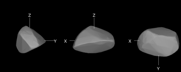
One of the new models – (1663) van den Bos – is particularly interesting because it has a very long rotation period of 748.7 hr, which is close to the synodic period of $740\pm 10$ hr determined by Stephens and Higgins (2011). Although we cannot rule out some excitation of its rotation state, it cannot be very high because we obtained a model with the same period and similar pole directions from inversion of an independent set of calibrated sparse data from the Lowell Photometric Database. The shape model for one of the possible poles is shown in Fig. 5.

This asteroid is an S-type, with the geometrical albedo $p_{V}=0.171\pm 0.018$ and diameter $D=(11.70\pm 0.05)\,{\rm km}$ (Masiero et al. 2011), The time scale of YORP-effect-driven evolution (or doubling time) can be estimated as:

\tau_{\rm YORP}=\tau_{0}c_{\rm YORP}^{-1}\left({a\over a_{0}}\right)^{\!2}\left({D\over D_{0}}\right)^{\!2}\left({\rho\over\rho_{0}}\right)\doteq 990\,{\rm Myr}\,,

where $\tau_{0}=11.9\,{\rm Myr}$ , $a_{0}=2.5\,{\rm au}$ , $D_{0}=2\,{\rm km}$ , $\rho_{0}=2\,500\,{\rm kg}\,{\rm m}^{-3}$ are the reference values from Čapek and Vokrouhlický (2004). Note that for decreasing the spin rate from an average value of $D=10\,{\rm km}$ asteroids, $\bar{\omega}\simeq 5\,{\rm rev}\,{\rm day}^{-1}$ , down to the current value, one would need about 7 doubling times.

At the same time, we can estimate a collisional reorientation time scale as:

\tau_{\rm reor}=B\left({\omega\over\omega_{0}}\right)^{\beta_{1}}\left({D\over D_{0}}\right)^{\beta_{2}}\doteq 140\,{\rm Myr}\,,

where we used $B=84.5\,{\rm kyr}$ , $\omega_{0}=2\pi/P_{0}$ , $P_{0}=5\,{\rm h}$ , $\beta_{1}=5/6$ , and $\beta_{2}=4/3$ according to Farinella et al. (1998). It means that the asteroid spin is currently rather driven by collisions than YORP. However, if the rotation was significantly faster in the past, the collisional time scale was most likely longer than $\tau_{\rm YORP}$ .

The time scale for damping of non-principal-axis rotation is of the order of (Hestroffer and Tanga 2006):

\tau_{\rm damp}={\mu Q\over\rho K_{1}^{2}(D/2)^{2}\omega^{3}}\simeq 10^{6}\,{\rm Myr}\,,

where we assumed $\rho=2\,500\,{\rm kg}\,{\rm m}^{-3}$ , $K_{1}^{2}\simeq 0.1$ , and the value $\mu Q=5\times 10^{12}\,{\rm Pa}$ (Harris 1994). In the current state, the damping thus seems negligible and from this point of view one would expect an excited state.

3 Conclusions

The new models we have obtained will further increase the number of asteroids for which a simple physical model exists. By building a database of such models, we can study the distribution of spins and shapes across the population. We will re-observe those targets, for which the current data sets are still not enough to build a unique model. The data obtained in the course of this project (together with other data) will be also used as independent observational constraints for dynamical models of asteroid families and their longer-term evolution, driven mostly by the Yarkovsky semimajor axis drift, chaotic diffusion in mean-motion resonances, eccentricity and inclination drift in secular resonances (Brož and Morbidelli 2013), random collisional reorientations, the YORP effect causing systematic changes of spin rates and spin poles (Hanuš et al. 2013), or even spin-orbital resonances (Vokrouhlický et al. 2003).

Luckily, the current number of shape models in DAMIT database seems sufficiently high, in order to focus on individual families. For example, recent census of the Eos family shows there are at least 43 core and 27 halo asteroids (including background) with known spin orientations (Hanuš et al., in prep.). There are three more Eos family members in our list of models. Together with distributions inferred from Lowell photometric data, in particular the absolute values of (approximate) pole latitudes $|\beta|$ for 69 053 asteroids (Cibulková et al. 2016), they may represent very stringent constraints for dynamics of small ( $D\simeq 10^{0}\,{\rm km}$ ) asteroids.

Acknowledgements

The work of MB and JĎ was supported by the Grant Agency of the Czech Republic (grant no. 15-04816S). The computations have been done on the computational cluster Tiger at the Astronomical Institute of Charles University in Prague (http://sirrah.troja.mff.cuni.cz/tiger). The development of the observatory was supported by the Technology Agency of the Czech Republic (TA ČR), project no. TA 03011171, ’Development of Technologies for the Fast Robotic Observatories and Laser Communication Systems’.

Table 1: Rotational states and light curve summary of asteroids, for which we derived their shape models. The table gives ecliptic coordinates

\lambda_{1}

\beta_{1}

\lambda_{2}

and

\beta_{2}

of the two best-fitting pole solutions, sidereal rotational period

P

, the number of dense light curves

N_{\mathrm{lc}}

spanning

N_{\mathrm{app}}

apparitions, the number of sparse-in-time measurements

N_{\mathrm{sp}}

, and the reference to the model.

Asteroid		$\lambda_{1}$	$\beta_{1}$	$\lambda_{2}$	$\beta_{2}$	$P$	$N_{\mathrm{lc}}$	$N_{\mathrm{app}}$	$N_{\mathrm{sp}}$	Reference
		[deg]	[deg]	[deg]	[deg]	[hours]
114	Kassandra	196	$-$ 55	4	$-$ 58	$10.74358$	24	8	322	This work
163	Erigone	191	$-$ 75	358	$-$ 73	$16.1403$	5	2	331	This work
		276	$-$ 69			$16.1402$			483	Ďurech et al. (2016)
176	Iduna	156	78	85	29	$11.28783$	9	3	360	This work
		219	68	83	24	$11.28785$			491	Ďurech et al. (2016)
582	Olympia	135	3			$36.3635$	104	6	443	This work
608	Adolfine	342	43	171	30	$8.34489$	10	3	224	This work
616	Elly	262	54	353	85	$5.29770$	19	3	284	This work
		250	44	60	62	$5.29770$			368	Ďurech et al. (2016)
775	Lumiere	89	54	248	47	$6.10300$	14	6	250	This work
822	Lalage	343	$-$ 74	133	$-$ 75	$3.346503$	13	3	445	This work
918	Itha	72	$-$ 54			$3.473808$	9	2	227	This work
		59	$-$ 59	249	$-$ 72	$3.47381$			350	Ďurech et al. (2016)
955	Alstede	64	57	246	23	$5.18734$	1	1	258	This work
		54	38	240	13	$5.18735$			401	Ďurech et al. (2016)
1095	Tulipa	142	40	349	56	$2.787153$	11	3	356	This work
1219	Britta	61	$-$ 62	223	$-$ 68	$5.57557$	21	3	231	This work
		72	$-$ 66	241	$-$ 66	$5.57556$			387	Ďurech et al. (2016)
1251	Hedera	271	$-$ 53	115	$-$ 62	$19.9020$	10	2	289	This work
		266	$-$ 62	124	$-$ 70	$19.9021$			414	Ďurech et al. (2016)
1320	Impala	186	$-$ 43	126	$-$ 70	$6.17081$	9	2	213	This work
		151	$-$ 57	254	$-$ 70	$6.17081$			353	Ďurech et al. (2016)
1380	Volodia	82	54	261	29	$6.19570$	1	1	197	This work
1663	van den Bos	248	62	43	51	$748.72$	37	2	241	This work
2511	Patterson	194	50	10	31	$4.14065$	1	1	164	This work
34817	Shiominemoto	201	36			$6.37750$	12	5	85	This work

Table 2: Light curve observations used for the shape model determinations. Our observations with the BE600 telescope were obtained by Martin Lehký.

Asteroid		Date	$N_{\mathrm{LC}}$	Observer/Telescope
114	Kassandra	1979 03 – 1980 07	2	Harris and Young (1989)
		1981 09 – 1981 09	2	Harris et al. (1992)
		1988 04 – 1988 04	3	Hutton and Blain (1988)
		1993 05 – 1993 05	2	Piironen et al. (1998)
		2006-6-24.0	1	Roberto Crippa, Federico Manzini
		2006-6-27.0	1	Roberto Crippa, Federico Manzini
		2006-6-30.0	1	Roberto Crippa, Federico Manzini
		2006-7-11.0	1	Roberto Crippa, Federico Manzini
		2006-7-21.0	1	Roberto Crippa, Federico Manzini
		2006-7-21.9	1	Roberto Crippa, Federico Manzini
		2006-8-06.9	1	Roberto Crippa, Federico Manzini
		2006-8-08.9	1	Roberto Crippa, Federico Manzini
		2011-8-29.9	1	René Roy
		2011-8-31.0	1	René Roy
		2011-9-17.0	1	René Roy
		2011-9-19.0	1	René Roy
		2016-08-02.1	1	Martin Lehký
		2016-08-14.0	1	Martin Lehký
		2016-08-18.0	1	Martin Lehký
163	Erigone	1980 12 – 1981 01	3	Harris and Young (1989)
		2016-11-20.8	1	Martin Lehký
		2016-12-29.8	1	Martin Lehký
176	Iduna	2007 09 – 2007 10	3	Warner (2008)
		2015-01-07.7	1	Julian Oey
		2015-01-14.7	1	Julian Oey
		2015-01-17.7	1	Julian Oey
		2015-01-23.5	1	Julian Oey
		2015-01-29.6	1	Julian Oey
		2016-04-29.9	1	Martin Lehký
582	Olympia	1986 01 – 1989 12	10	Schober et al. (1993)
		2006-11-13.6	1	Julian Oey
		2006-11-21.6	1	Julian Oey
		2013 05 – 2013 08	87	Pilcher et al. (2014)
		2016-04-30.0	1	Martin Lehký
		2016-04-30.9	1	Martin Lehký
		2016-05-02.9	1	Martin Lehký
608	Adolfine	2006-10-14.9	1	Raymond Poncy
		2006-10-24.9	1	Raymond Poncy
		2006-10-26.9	1	Raymond Poncy
		2006-10-27.9	1	Raymond Poncy
		2013-02-03.9	1	Roberto Crippa, Federico Manzini
		2006-10-11.0	1	Roberto Crippa, Federico Manzini
		2006-10-15.9	1	Roberto Crippa, Federico Manzini
		2006-10-26.9	1	Roberto Crippa, Federico Manzini
		2016-08-31.9	1	Martin Lehký
		2016-09-02.9	1	Martin Lehký
616	Elly	2010 01 – 2010 02	2	Warner (2010)
		2010 02 – 2010 02	2	Durkee (2010)
		2014 02 – 2014 02	2	Parnafes (2014)
		2014 02 – 2014 02	4	Stephens (2014)
		2014 02 – 2014 03	8	Klinglesmith et al. (2014)
		2016-10-04.8	1	Martin Lehký
775	Lumiere	1983 05 – 1983 05	3	Binzel (1987)
		2001-09-20.0	1	René Roy
		2001-09-26.0	1	René Roy
		2001-09-31.0	1	René Roy
		2001-08-27.1	1	René Roy
		2003-03-23.9	1	Claudine Rinner
		2005-07-07.1	1	Stephane Charbonnel, Pierre Dubreuil
				Alain Lopez, Gilles Kober
		2006-10-15.0	1	Raymond Poncy
		2006-10-24.9	1	Raymond Poncy
		2006-10-26.9	1	Raymond Poncy
		2006-10-27.8	1	Raymond Poncy
		2016-09-25.9	1	Martin Lehký
822	Lalage	1992 09 – 1992 09	2	Wisniewski et al. (1997)
		2009 10 – 2009 10	2	Higgins (2011)
		2014 01 – 2014 01	2	Stephens (2014)
		2014 02 – 2014 03	6	Klinglesmith et al. (2014)
		2016-12-29.0	1	Martin Lehký
918	Itha	2011 06 – 2011 06	4	Oey et al. (2012)
		2011 06 – 2011 07	3	Folberth et al. (2012)
		2016-08-24.0	1	Martin Lehký
		2016-12-03.8	1	Martin Lehký
955	Alstede	2016-03-17.9	1	Martin Lehký
1095	Tulipa	1983 02 – 1983 02	1	Binzel (1987)
		2005-04-15.0	1	Ondřejov
		2005-04-29.0	1	Ondřejov
		2005-04-28.0	1	Pierre Antonini, Raoul Behrend
		2005-05-15.0	1	Pierre Antonini, Raoul Behrend
		2005-05-26.9	1	Pierre Antonini, Raoul Behrend
		2005-05-32.0	1	Pierre Antonini, Raoul Behrend
		2005-06-02.0	1	Pierre Antonini, Raoul Behrend
		2005-06-01.9	1	Gino Farroni
		2005-05-32.0	1	Gino Farroni
		2016-06-24.0	1	Martin Lehký
1219	Britta	1983 09 – 1983 12	12	Binzel (1987)
		2014 01 – 2014 01	4	Stephens (2014)
		2014 02 – 2014 03	4	Klinglesmith et al. (2014)
		2016-10-30.9	1	Martin Lehký
1251	Hedera	2007 07 – 2007 10	9	Oey (2008)
		2016-08-08.0	1	Martin Lehký
1320	Impala	2006 05 – 2006 05	3	Warner (2006)
		2016 03 – 2016 04	5	Benishek (2016)
		2016-05-08.0	1	Martin Lehký
1380	Volodia	2016-09-24.0	1	Martin Lehký
1663	van den Bos	2010 09 – 2010 11	32	Stephens and Higgins (2011)
		2010 10 – 2010 11	4	Ruthroff (2011)
		2016-05-12.0	1	Martin Lehký
2511	Patterson	2016-12-03.9	1	Martin Lehký
34817	Shiominemoto	2003 07 – 2003 07	2	Warner (2004)
		2006 12 – 2006 12	2	Warner (2007)
		2011 11 – 2011 11	3	Warner (2012)
		2015 02 – 2015 02	4	Stephens (2015)
		2016-08-31.0	1	Martin Lehký

Table 2: continued.

Table 3: List of observers, their locations and telescope specifications.

Observer	Observatory	Telescope specification
Roberto Crippa	Tradate, Italy (B13)	Reflector 0.65m, F/D=5, Apogee Alta 1001, KAF-1001ME
Federico Manzini	Sozzago, Italy (A12)	D=0.40m F/D=5, Hisis 33
Martin Lehký	Ondřejov Observatory, Czech Republic (557)	BlueEye 600
René Roy	Observatoire de Blauvac, Blauvac, France (627)	D=0.312m, Hisis 22, KAF-400
Julian Oey	Kingsgrove, NSW, Australia (E19)	D=0.25m Schmidt-Cassegrain, F/D-5.2, SBIG ST-402ME CCD
Raymond Poncy	Le Crés Observatory, Le Crés, France (177)	D=0.20m F/D=3.3
Claudine Rinner	224 Ottmarsheim, France (224)	D=0.305m F/D=10, ST8e, KAF1602E, KAF3200me
Stephane Charbonnel	Observatoire de Durtal, Durtal, France (949)	D=0.30m, F/D=3.5, KAF-400e
Pierre Antonini	Observatoire des Hauts Patys, Bédoin, France (132)	D=0.305m, F/D=2.6 , NJP160, MCMT2, KAF-400

Table 3: continued.

References

Benishek (2016) Benishek, V., 2016. Lightcurves and Rotation Periods for 14 Asteroids. Minor Planet Bulletin 43, 339–342.
Binzel (1987) Binzel, R.P., 1987. A photoelectric survey of 130 asteroids. Icarus 72, 135–208.
Bowell et al. (2014) Bowell, E., Oszkiewicz, D.A., Wasserman, L.H., Muinonen, K., Penttilä, A., Trilling, D.E., 2014. Asteroid spin-axis longitudes from the Lowell Observatory database. Meteoritics and Planetary Science 49, 95–102. 1310.3617.
Brož and Morbidelli (2013) Brož, M., Morbidelli, A., 2013. The Eos family halo. Icarus 223, 844–849. 1302.1447.
Brož et al. (2013) Brož, M., Morbidelli, A., Bottke, W.F., Rozehnal, J., Vokrouhlický, D., Nesvorný, D., 2013. Constraining the cometary flux through the asteroid belt during the late heavy bombardment. Astronomy and Astrophysics 551, A117. 1301.6221.
Čapek and Vokrouhlický (2004) Čapek, D., Vokrouhlický, D., 2004. The YORP effect with finite thermal conductivity. Icarus 172, 526–536.
Cibulková et al. (2016) Cibulková, H., Ďurech, J., Vokrouhlický, D., Kaasalainen, M., Oszkiewicz, D.A., 2016. Distribution of spin-axes longitudes and shape elongations of main-belt asteroids. Astronomy and Astrophysics 596, A57. 1610.02790.
Ďurech et al. (2010) Ďurech, J., Sidorin, V., Kaasalainen, M., 2010. DAMIT: a database of asteroid models. Astronomy and Astrophysics 513, A46.
Ďurech et al. (2016) Ďurech, J., Hanuš, J., Oszkiewicz, D., Vančo, R., 2016. Asteroid models from the Lowell photometric database. Astronomy and Astrophysics 587, A48. 1601.02909.
Durkee (2010) Durkee, R.I., 2010. Asteroids Observed from the Shed of Science Observatory: 2009 October - 2010 March. Minor Planet Bulletin 37, 125–127.
Farinella et al. (1998) Farinella, P., Vokrouhlický, D., Hartmann, W.K., 1998. Meteorite Delivery via Yarkovsky Orbital Drift. Icarus 132, 378–387.
Folberth et al. (2012) Folberth, J., Casimir, S., Dou, Y., Evans, D., Foulkes, T., Haenftling, M., Kuhn, P., White, A., Ditteon, R., 2012. Asteroid Lightcurve Analysis at the Oakley Southern Sky Observatory: 2011 July-September. Minor Planet Bulletin 39, 51–55.
Hanuš et al. (2013) Hanuš, J., Brož, M., Ďurech, J., Warner, B.D., Brinsfield, J., Durkee, R., Higgins, D., Koff, R.A., Oey, J., Pilcher, F., Stephens, R., Strabla, L.P., Ulisse, Q., Girelli, R., 2013. An anisotropic distribution of spin vectors in asteroid families. Astronomy and Astrophysics 559, A134. 1309.4296.
Hanuš et al. (2016) Hanuš, J., Ďurech, J., Oszkiewicz, D.A., Behrend, R., Carry, B., Delbo, M., Adam, O., Afonina, V., Anquetin, R., Antonini, P., Arnold, L., Audejean, M., Aurard, P., Bachschmidt, M., Baduel, B., Barbotin, E., Barroy, P., Baudouin, P., Berard, L., Berger, N., Bernasconi, L., Bosch, J.G., Bouley, S., Bozhinova, I., Brinsfield, J., Brunetto, L., Canaud, G., Caron, J., Carrier, F., Casalnuovo, G., Casulli, S., Cerda, M., Chalamet, L., Charbonnel, S., Chinaglia, B., Cikota, A., Colas, F., Coliac, J.F., Collet, A., Coloma, J., Conjat, M., Conseil, E., Costa, R., Crippa, R., Cristofanelli, M., Damerdji, Y., Debackère, A., Decock, A., Déhais, Q., Déléage, T., Delmelle, S., Demeautis, C., Dróżdż, M., Dubos, G., Dulcamara, T., Dumont, M., Durkee, R., Dymock, R., Escalante del Valle, A., Esseiva, N., Esseiva, R., Esteban, M., Fauchez, T., Fauerbach, M., Fauvaud, M., Fauvaud, S., Forné, E., Fournel, C., Fradet, D., Garlitz, J., Gerteis, O., Gillier, C., Gillon, M., Giraud, R., Godard, J.P., Goncalves, R., Hamanowa, H., Hamanowa, H., Hay, K., Hellmich, S., Heterier, S., Higgins, D., Hirsch, R., Hodosan, G., Hren, M., Hygate, A., Innocent, N., Jacquinot, H., Jawahar, S., Jehin, E., Jerosimic, L., Klotz, A., Koff, W., Korlevic, P., Kosturkiewicz, E., Krafft, P., Krugly, Y., Kugel, F., Labrevoir, O., Lecacheux, J., Lehký, M., Leroy, A., Lesquerbault, B., Lopez-Gonzales, M.J., Lutz, M., Mallecot, B., Manfroid, J., Manzini, F., Marciniak, A., Martin, A., Modave, B., Montaigut, R., Montier, J., Morelle, E., Morton, B., Mottola, S., Naves, R., Nomen, J., Oey, J., Ogłoza, W., Paiella, M., Pallares, H., Peyrot, A., Pilcher, F., Pirenne, J.F., Piron, P., Polińska, M., Polotto, M., Poncy, R., Previt, J.P., Reignier, F., Renauld, D., Ricci, D., Richard, F., Rinner, C., Risoldi, V., Robilliard, D., Romeuf, D., Rousseau, G., Roy, R., Ruthroff, J., Salom, P.A., Salvador, L., Sanchez, S., Santana-Ros, T., Scholz, A., Séné, G., Skiff, B., Sobkowiak, K., Sogorb, P., Soldán, F., Spiridakis, A., Splanska, E., Sposetti, S., Starkey, D., Stephens, R., Stiepen, A., Stoss, R., Strajnic, J., Teng, J.P., Tumolo, G., Vagnozzi, A., Vanoutryve, B., Vugnon, J.M., Warner, B.D., Waucomont, M., Wertz, O., Winiarski, M., Wolf, M., 2016. New and updated convex shape models of asteroids based on optical data from a large collaboration network. Astronomy and Astrophysics 586, A108. 1510.07422.
Harris (1994) Harris, A.W., 1994. Tumbling asteroids. Icarus 107, 209.
Harris and Young (1989) Harris, A.W., Young, J.W., 1989. Asteroid lightcurve observations from 1979-1981. Icarus 81, 314–364.
Harris et al. (1992) Harris, A.W., Young, J.W., Dockweiler, T., Gibson, J., Poutanen, M., Bowell, E., 1992. Asteroid lightcurve observations from 1981. Icarus 95, 115–147.
Hestroffer and Tanga (2006) Hestroffer, D., Tanga, P., 2006. Asteroids from Observations to Models, in: Souchay, J. (Ed.), Dynamics of Extended Celestial Bodies and Rings, p. 89. astro-ph/0507158.
Higgins (2011) Higgins, D., 2011. Period Determination of Asteroid Targets Observed at Hunters Hill Observatory: May 2009 - September 2010. Minor Planet Bulletin 38, 41–46.
Hroch (1998) Hroch, F., 1998. Computer Programs for CCD Photometry, in: Dusek, J. (Ed.), 20th Stellar Conference of the Czech and Slovak Astronomical Institutes, p. 30.
Hutton and Blain (1988) Hutton, R.G., Blain, A., 1988. V+B Photoelectric Photometry of Asteroid 114 Kassandra. Minor Planet Bulletin 15, 39.
Kaasalainen and Lamberg (2006) Kaasalainen, M., Lamberg, L., 2006. Inverse problems of generalized projection operators. Inverse Problems 22, 749–769.
Kaasalainen et al. (2001) Kaasalainen, M., Torppa, J., Muinonen, K., 2001. Optimization methods for asteroid lightcurve inversion. II. The complete inverse problem. Icarus 153, 37–51.
Kim et al. (2014) Kim, M.J., Choi, Y.J., Moon, H.K., Byun, Y.I., Brosch, N., Kaplan, M., Kaynar, S., Uysal, Ö., Güzel, E., Behrend, R., Yoon, J.N., Mottola, S., Hellmich, S., Hinse, T.C., Eker, Z., Park, J.H., 2014. Rotational Properties of the Maria Asteroid Family. Astronomical Journal 147, 56. 1311.5318.
Klinglesmith et al. (2014) Klinglesmith, III, D.A., Hanowell, J., Risley, E., Turk, J., Vargas, A., Warren, C.A., 2014. Lightcurves for Inversion Model Candidates. Minor Planet Bulletin 41, 139–143.
Marciniak et al. (2015) Marciniak, A., Pilcher, F., Oszkiewicz, D., Santana-Ros, T., Urakawa, S., Fauvaud, S., Kankiewicz, P., Tychoniec, Ł., Fauvaud, M., Hirsch, R., Horbowicz, J., Kamiński, K., Konstanciak, I., Kosturkiewicz, E., Murawiecka, M., Nadolny, J., Nishiyama, K., Okumura, S., Polińska, M., Richard, F., Sakamoto, T., Sobkowiak, K., Stachowski, G., Trela, P., 2015. Against the biases in spins and shapes of asteroids. Planetary and Space Science 118, 256–266.
Masiero et al. (2011) Masiero, J.R., Mainzer, A.K., Grav, T., Bauer, J.M., Cutri, R.M., Dailey, J., Eisenhardt, P.R.M., McMillan, R.S., Spahr, T.B., Skrutskie, M.F., Tholen, D., Walker, R.G., Wright, E.L., DeBaun, E., Elsbury, D., Gautier, I.T., Gomillion, S., Wilkins, A., 2011. Main Belt Asteroids with WISE/NEOWISE. I. Preliminary Albedos and Diameters. Astrophysical Journal 741, 68. 1109.4096.
Nesvorný (2012) Nesvorný, D., 2012. Nesvorny HCM Asteroid Families V2.0. NASA Planetary Data System 189.
Nesvorný (2015) Nesvorný, D., 2015. Nesvorny HCM Asteroid Families V3.0. NASA Planetary Data System 234.
Nesvorný et al. (2015) Nesvorný, D., Brož, M., Carruba, V., 2015. Identification and Dynamical Properties of Asteroid Families, in: Michel, P., DeMeo, F.E., Bottke, W.F. (Eds.), Asteroids IV. University of Arizona Press, Tucson, pp. 297–321.
Oey (2008) Oey, J., 2008. Lightcurve Analysis of Asteroids from the Kingsgrove and Leura Observatories in the 2nd Half of 2007. Minor Planet Bulletin 35, 132–135.
Oey et al. (2012) Oey, J., Colazo, C., Mazzone, F., Chapman, A., 2012. The Lightcurve Analysis of 918 Itha and 2008 Konstitutsiya. Minor Planet Bulletin 39, 1–2.
Oszkiewicz et al. (2011) Oszkiewicz, D., Muinonen, K., Bowell, E., Trilling, D., Penttilä, A., Pieniluoma, T., Wasserman, L., Enga, M.T., 2011. Online multi-parameter phase-curve fitting and application to a large corpus of asteroid photometric data. Journal of Quantitative Spectroscopy and Radiative Transfer 112, 1919–1929. Electromagnetic and Light Scattering by Nonspherical Particles {XII}.
Parnafes (2014) Parnafes, R., 2014. Photometric study and 3d modeling of two asteroids using inversion techniques. Research work done via the Bareket observatory, Israel.
Piironen et al. (2001) Piironen, J., Lagerkvist, C., Torppa, J., Kaasalainen, M., Warner, B., 2001. Standard Asteroid Photometric Catalogue, in: Bulletin of the American Astronomical Society, p. 1562.
Piironen et al. (1998) Piironen, J., Lagerkvist, C.I., Erikson, A., Oja, T., Magnusson, P., Festin, L., Nathues, A., Gaul, M., Velichko, F., 1998. Physical studies of asteroids. XXXII. Rotation periods and UBVRI-colours for selected asteroids. Astronomy and Astrophysics Supplement Series 128, 525–540.
Pilcher et al. (2014) Pilcher, F., Ferrero, A., Franco, L., Oey, J., Warner, B.D., 2014. A Photometric Study of 582 Olympia. Minor Planet Bulletin 41, 22–23.
Ruthroff (2011) Ruthroff, J.C., 2011. Lightcurve Analysis of Eight Main-belt Asteroids and a Revised Period for 185 Eunike. Minor Planet Bulletin 38, 86–88.
Schober et al. (1993) Schober, H.J., Erikson, A., Hahn, G., Lagerkvist, C.I., Oja, T., 1993. Physical Studies of Asteroids. Part XXVI. Rotation and Photoelectric Photometry of Asteroids 323, 350, 582, 1021 and 1866. Astronomy and Astrophysics Supplement Series 101, 507.
Slivan et al. (2009) Slivan, S.M., Binzel, R.P., Kaasalainen, M., Hock, A.N., Klesman, A.J., Eckelman, L.J., Stephens, R.D., 2009. Spin vectors in the Koronis family. II. Additional clustered spins, and one stray. Icarus 200, 514–530.
Snodgrass and Carry (2013) Snodgrass, C., Carry, B., 2013. Automatic Removal of Fringes from EFOSC Images. The Messenger 152, 14–16.
Stephens (2014) Stephens, R.D., 2014. Asteroids Observed from CS3: 2014 January - March. Minor Planet Bulletin 41, 171–175.
Stephens (2015) Stephens, R.D., 2015. Asteroids Observed from CS3: 2015 January - March. Minor Planet Bulletin 42, 200–203.
Stephens and Higgins (2011) Stephens, R.D., Higgins, D., 2011. The Lightcurve for the Long-period Asteroid 1663 van den Bos. Minor Planet Bulletin 38, 72.
Stetson (2011) Stetson, P.B., 2011. DAOPHOT: Crowded-field Stellar Photometry Package. Astrophysics Source Code Library. 1104.011.
Vokrouhlický et al. (2003) Vokrouhlický, D., Nesvorný, D., Bottke, W.F., 2003. The vector alignments of asteroid spins by thermal torques. Nature 425, 147–151.
Warner (2004) Warner, B.D., 2004. Rotation rates for asteroids 875, 926, 1679, 1796, 3915, 4209, and 34817. Minor Planet Bulletin 31, 19–22.
Warner (2006) Warner, B.D., 2006. Asteroid lightcurve analysis at the Palmer Divide Observatory - March - June 2006. Minor Planet Bulletin 33, 85–88.
Warner (2007) Warner, B.D., 2007. Asteroid Lightcurve Analysis at the Palmer Divide Observatory - September-December 2006. Minor Planet Bulletin 34, 32–37.
Warner (2008) Warner, B.D., 2008. Asteroid Lightcurve Analysis at the Palmer Divide Observatory - June - October 2007. Minor Planet Bulletin 35, 56–60.
Warner (2010) Warner, B.D., 2010. Asteroid Lightcurve Analysis at the Palmer Divide Observatory: 2009 December - 2010 March. Minor Planet Bulletin 37, 112–118.
Warner (2012) Warner, B.D., 2012. Asteroid Lightcurve Analysis at the Palmer Divide Observatory: 2011 September - December. Minor Planet Bulletin 39, 69–80.
Warner et al. (2016) Warner, B.D., Harris, A.W., Durech, J., Benner, L.A.M., 2016. Lightcurve Photometry Opportunities: 2016 October-December. Minor Planet Bulletin 43, 356–361.
Warner et al. (2009) Warner, B.D., Harris, A.W., Pravec, P., 2009. The asteroid lightcurve database. Icarus 202, 134–146.
Warner et al. (2011) Warner, B.D., Stephens, R.D., Harris, A.W., 2011. Save the Lightcurves. Minor Planet Bulletin 38, 172–174.
Wisniewski et al. (1997) Wisniewski, W.Z., Michałowski, T.M., Harris, A.W., McMillan, R.S., 1997. Photometric Observations of 125 Asteroids. Icarus 126, 395–449.
Zacharias et al. (2013) Zacharias, N., Finch, C.T., Girard, T.M., Henden, A., Bartlett, J.L., Monet, D.G., Zacharias, M.I., 2013. The Fourth US Naval Observatory CCD Astrograph Catalog (UCAC4). Astronomical Journal 145, 44. 1212.6182.