Spectral analysis of gravitational waves from binary neutron star merger remnants
Abstract
In this work we analyze the gravitational wave signal from hypermassive neutron stars formed after the merger of binary neutron star systems, focusing on its spectral features. The gravitational wave signals are extracted from numerical relativity simulations of models already considered by De Pietri et al. [Phys. Rev. D 93, 064047 (2016)], Maione et al. [Classical Quantum Gravity 33, 175009 (2016)], and Feo et al. [Classical Quantum Gravity 34, 034001 (2017)], and allow us to study the effect of the total baryonic mass of such systems (from to ), the mass ratio (up to ), and the neutron star equation of state, both in equal and highly unequal mass binaries. We use the peaks we find in the gravitational spectrum as an independent test of already published hypotheses of their physical origin and empirical relations linking them with the characteristics of the merging neutron stars. In particular, we highlight the effects of the mass ratio, which in the past was often neglected. We also analyze the temporal evolution of the emission frequencies. Finally, we introduce a modern variant of Prony’s method to analyze the gravitational wave postmerger emission as a sum of complex exponentials, trying to overcome some drawbacks of both Fourier spectra and least-squares fitting. Overall, the spectral properties of the postmerger signal observed in our simulation are in agreement with those proposed by other groups. More specifically, we find that the analysis of Bauswein and Stergioulas [Phys. Rev. D 91, 124056 (2015)] is particularly effective for binaries with very low masses or with a small mass ratio and that the mechanical toy model of Takami et al. [Phys. Rev. D 91, 064001 (2015)] provides a comprehensive and accurate description of the early stages of the postmerger.
pacs
04.25.D-, 04.40.Dg, 95.30.Lz, 97.60.JdI Introduction
Gravitational waves (GW) from binary neutron star (BNS) mergers are the next target for Earth-based interferometric detectors, after the recent first detection of GW from two binary black hole mergers [1, 2, 3]. BNSs are a particularly interesting system to study, since they are also linked to the electromagnetic signal counterpart to the GWs [4, 5, 6, 7], to be the center for r-process nucleosynthesis in material that is dynamically ejected [8, 9] macronovae [10, 11, 12, 13, 14, 15, 16] from the material ejected during and after the merger, and are related to short gamma ray bursts [17, 18, 19, 20] (whose central engine mechanism is still disputed). Even more importantly, BNS mergers can be thought as a laboratory to study nuclear physics at the extreme conditions present in neutron star cores [21]. The still unknown equation of state (EOS) of nuclear matter inside the neutron star core, at densities higher than at nuclear equilibrium, will leave an imprint on the GW signal emitted both before and after the merger.
For the coalescent phase, semi-analytic techniques have been developed that include effects due to the tidal deformability effect of matter EOS, in particular within the effective-one-body (EOB) formalism [22, 23, 24, 25], and tested and validated using numerical relativity (see for example [26, 27, 28, 29]). On the other hand, for the merger and postmerger phase, numerical relativity is the only available tool to study the evolution of the remnant and its GW emission, in the case in which a (hyper)massive neutron star [30], or a black hole surrounded by an accretion disk is formed. If a neutron star remnant is produced, its GW emission will still be linked to the neutron star EOS. In particular, many recent works focused on linking the spectral peaks of postmerger GW emission with some characteristics of the merging neutron stars [31, 32, 33, 34, 35, 36, 37, 13, 38, 39, 40], such as their radius, compactness or tidal deformability. If the progenitor masses would be known from the inspiral signal, they could be used to constrains the EOS together with information about the postmerger peaks.
Despite this large body of previous works, which mainly focuses on constructing empirical relations between GW spectral features and EOS-related features, there is still an open debate about the physical origin of the postmerger GW signal, especially the subdominant spectral peaks.
In this work, we analyze the postmerger GW signal from numerical relativity simulations, of which other aspects were already highlighted our previous works [41, 42, 43]. Our goals here are to get a clearer picture of the postmerger GW emission mechanisms and their evolution in time, and to act as an independent test for empirical relations published in the recent literature, which are often tested only on the same data used to derive them. Our set of simulations spans several directions in the relevant parameter space, investigating the effect of the total baryonic mass (from of model SLy 1.11vs1.11 to of model SLy 1.44vs1.44), the mass ratio (up to , which corresponds to the largest mass asymmetry observed in a BNS system in our galaxy [44]), and the high density EOS in both equal and highly unequal mass systems. In particular, unequal mass systems were less widely investigated for the effect of the mass ratio in the postmerger GW analysis [32, 41, 45, 39, 46]. In this work we will highlight the effect of mass-ratio on the GW spectral features and evaluate the error of applying empirical relations developed for equal or close-to-equal mass binaries to highly unequal mass ones. The presence of this effect was already emphasized in [13] for the existence of empirical relations between the peak frequency of the GW signal and the radius of the neutron star.
We also adopt, for the first time, a modern version of Prony’s method [47, 48, 49, 50, 51] to analyze GWs from BNS merger remnants. It is a promising technique, since it is able to overcome some of the limitations of both Fourier spectrograms and least-squares fitting. In particular, the Prony analysis allows us to confirm that the postmerger GW signal is given by a sum of complex exponential modes, which could not be clearly identified from the Fourier spectra alone. We also validate those mode frequencies and their time evolution with an independent data analysis technique.
The paper is organized as follows: in section II we briefly describe the simulated initial data and the numerical methods adopted. In section III we present the results of our analysis. In particular, III.4 contains a comparison of some empirical relations for the dominant spectral peaks with our data, in section III.5 we discuss different models for explaining the subdominant peaks in the spectra, before we introduce the version of the Prony’s method we implemented and the results obtained applying it to our data in section III.6. Finally, we conclude our analysis in section IV. The work is completed by one appendix A, containing characteristics of our initial data, as well as a comparison of our data with existing, universal formulas for the postmerger peak frequencies.
Throughout this paper we use a spacelike signature , with Greek indices running from 0 to 3, Latin indices from 1 to 3, and the standard convention for summation over repeated indices. The computations are performed using the standard split into (usually) spacelike coordinates and a time-like coordinate . Our coordinate system (far-from the origin) are, as it can be checked, almost isotropic coordinates and (far-from the origin) they would have the usual measure unit of “time” and “space” and in particular is close to be identified as the time measured from an observer at infinity.
All computations have been done in normalized computational units (hereafter denoted as CU) in which . We report all results in cgs units except for values of the polytropic constant , whose unit of measurement depends on the value of the dimensionless polytropic exponent , so we report in the above defined normalized unit CU). We also report masses in terms of the solar mass . The reader should note that, as is usual in most of the work on this subject we describe matter using the variable (baryon mass density), (specific internal energy) and , instead of, as usually used in Astrophysics, (energy density), (baryon number density) and . Their relation is the following: and ( is the baryon mass).
II Initial Models and Numerical Methods
The models analyzed in this paper were already considered in our previous works [41, 42, 43] where a detailed discussion of the employed numerical methods, their convergence properties as well as of their properties can be find. We report here the general simulation setup and parameters and refer to those previous articles for simulation setup details. In particular, the resolution used in the simulation here presented ( CU m) is coarser than the one used in other works but that should not efffect the identification of the peaks (see [41] for a discussion of the convergence properties of the code).
The simulations were performed using the Einstein Toolkit [52], an open source, modular code for numerical relativity based on the Cactus framework [53, 54]. The evolved variables were discretized on a Cartesian grid with 6 levels of fixed mesh refinement, each using twice the resolution of its parent level. The outermost face of the grid was set at ( km) from the center. We solved the BSSN-OK formulation of Einstein’s equations [55, 56, 57, 58, 59], implemented in the McLachlan module [60], and the general relativistic hydrodynamics equations (GRHD) with High resolution shock capturing methods, implemented by the public GRHydro module [61, 62]. In particular, we used a finite-volume algorithm with the HLLE Riemann solver [63, 64] and the WENO reconstruction method [65, 66]. The combined use of WENO reconstruction and the BSSN-OK formulation was found in [41] to be the best combination within the Einstein Toolkit even at low resolution in [41]. For time evolution, we used the Method of Lines, with fourth-order Runge-Kutta [67, 68].
Initial data were generated with the LORENE code [69, 70], as irrotational binaries in the conformal thin sandwich approximation. In this work we analyze a set of simulations with the SLy EOS [70] (from ref. [41]), equal mass systems with total baryonic mass from to and unequal mass systems with the same total baryonic mass and mass ratio up to . We also study simulations with different EOSs, both in equal mass systems (with total mass , from ref. [42]) and unequal mass binaries, simulating the merger of the observed system PSR J0453+1559 (see ref. [43]), the BNS system with the largest mass asymmetry observed so far in our galaxy [44]. The simulations from ref. [41] have an initial distance between the merging stars of km, while it was set to km for the simulations from ref. [42, 43]. More physical initial data characteristics are reported in the Appendix.
The cold part of the EOS is parametrized as a piecewise polytrope with 7 pieces, following the prescription of ref. [71]:
| (1) | ||||
| (2) |
where and are fixed imposing the continuity of the zero-temperature pressure and the specific energy density ( and respectively), starting from , and the (zero-temperature) pressure value at the fixed density . The four lowest-density pieces are common to all the adopted EOS, and are taken from the SLy EOS [72]. The three high density pieces, instead, differ for the four EOS models we compared (two nuclear many-body EOSs, SLy [73] and APR4 [74], and two relativistic mean-filed EOSs, H4 [75] and MS1 [76]). All the EOS-specific parameters are reported in table 1. During the evolution, the cold EOS is supplemented by an ideal-fluid thermal component, to ensure thermodynamic consistency in the presence of shocks. It takes the form of a -law, with the choice [77].
| (3) |
| i | |||||
|---|---|---|---|---|---|
| APR4 | SLy | H4 | MS1 | ||
| 0 | - | 1.584 | |||
| 1 | 1.287 | ||||
| 2 | 0.622 | ||||
| 3 | 1.357 | ||||
| 4 | 2.830 | 3.005 | 2.909 | 3.224 | |
| 5 | 3.445 | 2.988 | 2.246 | 3.033 | |
| 6 | 3.348 | 2.851 | 2.144 | 1.325 | |
II.1 Gravitational waves extraction
During the simulations the GW signal is extracted computing the Newman-Penrose scalar [78, 79] (using the code module WeylScalar4), which is linked to the GW strain by the following relation, valid only at spatial infinity:
| (4) |
where and are the two polarizations of the complex GW strain . The signal is then decomposed in spin-weighted spherical harmonics of weight [80] (by the module Multipole):
| (5) |
Since in this work we only focus on the dominant mode, we will identify for the rest of this paper. In order to get the GW strain form and minimizing the extraction errors, one has to extrapolate the signal extracted within the simulation at finite distance from the source to infinity, in order for eq. (4) to be valid. Then, the extrapolated is integrated twice in time, employing an appropriate technique to reduce the amplitude oscillations caused by high-frequency noise aliased in the low-frequency signal and amplified by the double integration process [81]. We adopted the procedure developed and extensively discussed in ref. [42]: first, is extrapolated to spatial infinity using the second order perturbative correction of Nakano and collaborators [82]:
| (6) | ||||
Both the GW strains at finite radius, which are present in eq. (6), and the final extrapolated strain are computed first by integrating the Newman-Penrose scalar twice in time with a simple trapezoid rule, starting from zero coordinate time, and fixing only the two physically meaningful integration constants and by subtracting a linear fit of itself from the signal:
| (7) | ||||
| (8) |
Only after the integration, a digital high-pass Butterworth filter is applied, designed to have a maximum amplitude reduction of dB at the initial GW frequency (assumed to be two times the initial orbital angular velocity, as reported by the LORENE code), and an amplitude reduction of dB at frequency .
All the GW related information will be reported in function of the retarded time
| (9) | ||||
From the GW strain obtained with the aforementioned procedure, we arrive at the GW amplitude spectral density , which is the physical observable we are focusing on in the analysis presented in this work, with:
| (10) |
where is the Fourier transform of the complex GW strain:
| (11) |
III Results
In order to study the spectral features of GWs emitted by the hypermassive neutron star remnant after the merger of BNS systems, we first compute the whole Fourier spectrum, as described in the previous section, from ms before up to ms after merger. The results are shown in figure 1. For all models, the spectrum has an initial growth and a maximum (corresponding to the inspiral GW emission, which has finite temporal length). The filled circles in figure 1 mark the instantaneous frequency at merger, computed as , where is taken as the time at which the GW amplitude is maximum, and is the accumulated GW phase, with the integer chosen to impose its continuity. The segment of each spectrum at frequencies greater than the merger frequency is generated by the merger remnant GW emission. In particular, for all models, it shows a well known dominant peak. This peak corresponds to the frequency (also called or in the literature), of the fundamental quadrupolar oscillation mode of the bar-deformed neutron star formed after the merger [33]. Its frequency has been correlated with different characteristics of the merging neutron stars [31, 32], in particular for constructing empirical relations to constrains the neutrons star EOS with future BNS postmerger GW detections. For a quantitative discussion of some of those relations, see sec. III.4. Most models also show one or more subdominant peaks, at frequencies both lower and higher than the dominant one. The scientific debate about their physical origin is still open (see ref. [13, 40] for an overview of the most recent results). Like the dominant peak, especially the low-frequency subdominant peak has been the target for empirical relations linking it to the characteristics of static stars with the same EOS as that of the merger remnant. A detailed discussion about subdominant peaks is presented in section III.5. Looking at figure 1, one can have a first qualitative impression about the dependency of the spectral features on the total mass of the binary, the mass ratio, and the neutron star EOS. In the top-left panel, equal mass systems with the same EOS (SLy) and different total mass are compared. With increasing mass, the dominant peak gains more power and moves towards higher frequencies, as it is expected from a more compact remnant. For most models, there are two subdominant peaks which are about equidistant from the dominant peak. They also gain more power with increasing total mass. As an exception, there is no recognizable peak with a frequency higher than the dominant one for the system SLy 1.11bs1.11 with . The highest-mass system considered (, model SLy 1.36vs1.36, which collapses to black-hole ms after the merger) instead, shows an additional low frequency peak, which does not correspond to any of the emission mechanisms analyzed so far in the literature. It is situated at a lower frequency than the merger one, but it comes, nevertheless, from the postmerger, as confirmed by the spectrogram (see later in the text and figure 2). The top-right panel shows unequal mass systems with the same total baryonic mass () and EOS (SLy), but different mass ratios, up to . As already reported in ref. [41] and confirmed in other works published in the past year [39, 46], the mass asymmetry leads to a lower dominant peak frequency and subdominant peaks with progressively less power. The bottom panels show the EOS effects for unequal (left) and equal (right) mass binaries: the softest EOSs (SLy and APR4), which lead to the most compact remnants, are characterized by a dominant peak at higher frequencies (therefore, more difficult to detect in current generation GW interferometers). The low-frequency subdominant peaks have relatively higher power for the less compact stars (H4 and, in a more pronounced fashion, MS1), while a high frequency subdominant peak is clearly recognizable only in the most compact stars. This difference was already noted in the unified model of [37], and was being attributed to the possibility of different emission mechanisms being responsible for the subdominant spectral peaks in soft and stiff EOS stars (see section III.5 for a deeper discussion about this hypothesis).
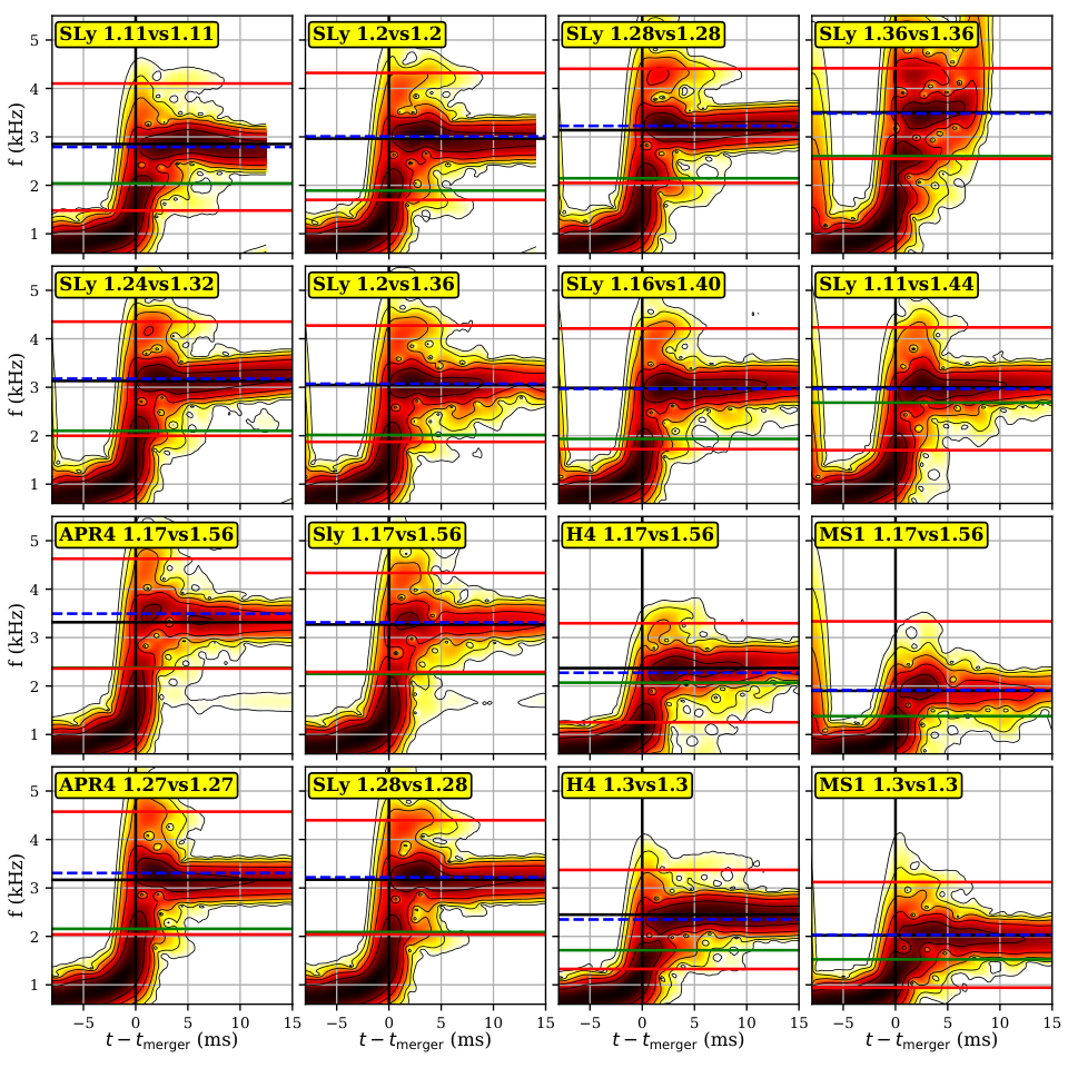
References. [84, 40, 46] highlighted the importance of not only analyzing the spectrum taken over the entire merger time, but also analyzing its time evolution. This is important, because the signal components are not fixed in time, but their frequencies evolve dynamically. Figure 2 shows the GW Fourier spectrogram for all the analyzed models, computed taking the Fourier transform in intervals of ms, with a superposition of 95%. Before the Fourier transform, the time domain signal is first padded with zeros to obtain a better frequency resolution, with a padding length of twice the length of the original signal. The first qualitative information noticeable in the spectrograms is that the subdominant modes are short lived, and that they decay during the first ms after merger. Even if they are too weak to be fully visible in the spectrograms, all the subdominant modes are active just after the merger. For unequal mass systems with a soft EOS this show that the main emission mechanism is only suppressed by the mass asymmetry, but it is nevertheless active. Finally, the dominant emission peak does not show a fixed frequency, but changes slightly with time.
In the following subsections we present the results obtained for the descriptions of the postmerger spectrum of binary neutron star mergers.
III.1 Rapid change of within few ms after merger
The frequency of the main emission mode rapidly changes in the first milliseconds after the merger, when also the subdominant modes are active, and when the merger remnant is rapidly evolving toward a more stable, equilibrium configuration. This feature was already noted in ref. [40] and was described using the notation to indicate a short-lived mode that evolves into the frequency. This continuous process seems to have different characteristics depending on the binary physical characteristics as was observed in the spectrogram of [84]. For example, in some models this frequency change is a slow process, with the dominant frequency first increasing (after the merger) and then decreasing, to reach its quasistationary stage value, as happens for the equal mass SLy EOS model (top-left panel), or for the equal mass model with the H4 EOS (third panel of the bottom row). In other systems this maximum in the dominant frequency is also present, but the quasi-stationary phase is reached much more quickly, as the equal mass systems with the SLy EOS and (second and third panels in the first row) or all the systems with the parameter of the observed PSR J0453+1559 binary (third row). Finally, there are systems for which the dominant frequency just decreases from its value right after the merger to the quasistationary phase value (like the equal mass APR4 model). It is interesting to note that in the PSR J0453+1559 system with a soft EOS (SLy or APR4), the change in frequency of the dominant peak is visible also in the full spectrum (figure 1, bottom-left panel), as the splitting of the main peak, and as already reported in [43]. Although this could be considered an artifact of the short post merger simulated time, it is unlikely to change even for a longer observation period. The reason is that it is caused by the fact that the GW amplitude quickly decreases after the first transient phase in high mass asymmetry models, allowing for the short but with relative high amplitude transient emission to leave an imprint on the overall spectrum as a local maximum, which does not happen in equal or close-to-equal mass binaries, where the GW emission amplitude decreases more slowly in the quasi-stationary phase.
III.2 Slow increase of at late times
The dominant mode frequency, in the last part of the signal, when it is the only active component, increases with time in most models. This effect is expected, because the angular momentum emitted in GW and redistributed by hydrodynamical processes drives the merger remnant to be more axisymmetric (damping the amplitude of the GW emission) and more compact (increasing its frequency). This frequency increase is more pronounced in models with higher total mass (see first row of fig. 2) and in equal mass models, while highly unequal mass ones show little or no frequency change in the temporal interval considered in this work, independently from the EOS (see third row). This is quite easy to understand, since the remnants of unequal mass binary mergers are less compact, and, in particular, more matter is ejected far from its core due to the tidal deformation of the lower mass star by its companion gravitational field which begins in the last orbits before the merger.
III.3 Other features
Finally, other subdominant modes are visible from the spectrograms, which are not explained by any of the standard pictures published so far, like the already mentioned low-frequency peak in the collapsing model SLy1.36vs1.36, which is generated at merger and lasts for the first ms, or the extended low frequency emissions around kHz visible in the PSR J0453+1559 system with the APR4 or EOSs, which start to develop about ms after the merger, already noticed and discussed in ref. [43].
III.4 The dominant emission frequency and its link with the stellar properties
| Model | [13] | [39] | ||||
|---|---|---|---|---|---|---|
| [kHz] | [kHz] | [kHz] | [km] | [kHz] | ||
| SLy | 1.11vs1.11 | 2.79 | 2.85 | 2.784 | 0.16 | 2.83 |
| SLy | 1.20vs1.20 | 3.01 | 2.96 | 3.009 | 0.10 | 3.03 |
| SLy | 1.28vs1.28 | 3.23 | 3.14 | 3.212 | 0.15 | 3.20 |
| SLy | 1.36vs1.36 | 3.48 | 3.51 | 3.410 | 0.19 | 3.38 |
| SLy | 1.24vs1.32 | 3.18 | 3.13 | 3.210 | 0.17 | 3.20 |
| SLy | 1.20vs1.36 | 3.07 | 3.05 | 3.210 | 0.35 | 3.20 |
| SLy | 1.16vs1.40 | 2.97 | 2.98 | 3.210 | 0.49 | 3.20 |
| SLy | 1.11vs1.44 | 2.97 | 3.00 | 3.197 | 0.43 | 3.20 |
| APR4 | 1.17vs1.56 | 3.49 | 3.32 | 3.574 | 0.50 | 3.67 |
| SLy | 1.17vs1.56 | 3.31 | 3.27 | 3.427 | 0.31 | 3.41 |
| H4 | 1.17vs1.56 | 2.27 | 2.37 | 2.503 | 0.44 | 2.25 |
| MS1 | 1.17vs1.56 | 1.91 | 1.90 | 2.179 | 2.30 | 1.88 |
| APR4 | 1.27vs1.27 | 3.31 | 3.17 | 3.336 | 0.35 | 3.47 |
| SLy | 1.28vs1.28 | 3.22 | 3.17 | 3.212 | 0.08 | 3.20 |
| H4 | 1.30vs1.30 | 2.35 | 2.45 | 2.382 | 0.21 | 2.12 |
| MS1 | 1.30vs1.30 | 2.03 | 2.02 | 2.081 | 0.29 | 1.80 |
The physical mechanism behind to the dominant peak in the postmerger GW spectrum is well known and agreed upon in the literature. As anticipated in the Introduction, several empirical relations have been developed to link the peak frequency with the merging star characteristics, like their radii [85, 86, 36, 13], compactness [87, 35, 39], or tidal deformability [34, 38, 40, 88]. One of the purposes of this work is to use our data, which cover a relevant portion of the expected BNS parameter space, as an independent test for such relations, in order to check their validity and estimation error on a set of simulations different from the ones used to obtain the relation parameters with nonlinear fitting.
In particular, we started form the results of ref. [89], which state that for equal mass models, correlates tightly with the radius of a static neutron star in equilibrium with the same EOS and a mass higher than the mass of each merging star. In particular, the dominant postmerger emission frequency from a system with two stars was correlated with the radius of a static star of . In ref. [13] [Eq. (2)], a relationship which connects the radius of a static TOV star with the frequency and the total gravitational mass [see Eq. (55) in Appendix A for ] of the merging system was also presented, but was reported to have higher errors in the obtained radii with respect to the fixed-total-mass relations. However, it is important to keep in mind that the authors in [13] already noted that for an unequal mass merger, such a relation it is not naturally fulfilled. We compared the aforementioned relation with our data of systems with varying total gravitational mass. The result of such a comparison are reported in table 2, together with the corresponding errors in the obtained radii. The radii of TOV stars of mass are computed for each EOS using the rns code [90].
We want to stress that eq. (2) of [13], like most empirical relationships of this kind so far, does not take mass ratio effects into account. According to our results, this can cause an error in the inferred radius of the order of m for the largest mass asymmetries observed in double neutron star systems. To take the mass ratio into account, a new relation was developed in [39], correlating linearly with the stars contact frequency, which is sensible to the mass ratio and can be obtained, to first approximation, from the stars’ masses and compactness [91]. Results shown in table 2 show, however, that the dependency between contact frequency and mass ratio seems to be too weak to fully account for the differences observed in , as was already observed in figure 4 in ref. [39]. In essence, this simpler and physically motivated empirical relation, seems to perform worse on our data than the correlation with the radius of a static star.
III.5 Physical interpretation and correlations of the subdominant frequencies
| Model | |||||
|---|---|---|---|---|---|
| [kHz] | [kHz] | [kHz] | [kHz] | ||
| SLy | 1.11vs1.11 | 2.04 | - | 1.31 | 1.72 |
| SLy | 1.20vs1.20 | 1.89 | 4.17 | 1.31 | 1.81 |
| SLy | 1.28vs1.28 | 2.15 | 4.30 | 1.19 | 1.91 |
| SLy | 1.36vs1.36 | 2.60 | 4.30 | 0.93 | 1.98 |
| SLy | 1.24vs1.32 | 2.10 | 4.26 | 1.18 | 1.90 |
| SLy | 1.20vs1.36 | 2.01 | 4.19 | 1.20 | 1.82 |
| SLy | 1.16vs1.40 | 1.93 | 4.11 | 1.24 | 1.73 |
| SLy | 1.11vs1.44 | - | - | 1.27 | 1.63 |
| APR4 | 1.17vs1.56 | 2.38 | 4.62 | 1.13 | 1.87 |
| SLy | 1.17vs1.56 | 2.25 | 4.23 | 1.02 | 1.67 |
| H4 | 1.17vs1.56 | - | - | 1.02 | 1.27 |
| MS1 | 1.17vs1.56 | - | - | 1.42 | 1.18 |
| APR4 | 1.27vs1.27 | 2.16 | 4.48 | 1.27 | 1.96 |
| SLy | 1.28vs1.28 | 2.12 | 4.35 | 1.18 | 1.87 |
| H4 | 1.30vs1.30 | 1.71 | - | 1.02 | 1.45 |
| MS1 | 1.30vs1.30 | 1.52 | - | 1.09 | 1.32 |
In the literature have been proposed various explanations for the subdominant peaks and (also called and ) which appear in the spectrum of postmerger GW emission in most BNS models.
The first hypothesis but forward was to consider them as the result of the combinations of the quasi radial oscillation mode and the fundamental mode [33] . In most models, the subdominant peaks are almost equidistant from the dominant one. The red horizontal lines in figure 2, and the corresponding vertical lines in figure 3, showing on each panel the GW spectrum of a single model, are drawn at frequencies , which are the theoretical frequencies of the mode combination. Here , adopting the notation of [40], is the dominant frequency in the first milliseconds after the merger, evaluated taking the maximum of the amplitude spectral density computed up to ms after the merger. , instead, is the frequency of the quasi-radial oscillations, computed from the spectrum of the maximum density (or minimum lapse) oscillations (see figure 5). In most models the frequency predicted for the mode combination is a very good approximation for the subdominant peaks in the spectrum. However, it is significantly different in the less compact stars, either low mass models with a soft EOS (such as the equal mass model with the SLy EOS and for each star, top-left panel in figure 3), or models with a stiff EOS (such as the stars with and the H4 or MS1 EOS).
Before addressing the mode combination interpretation in the less compact stars one should consider that in [87, 35, 92] was hypothesized and analyzed the possibility that all the subdominant peaks are generated by the modulation of the dominant mode due to the radial oscillation of the rotating double core structure formed right after the merger and that this modulation could be described by a mechanical toy model [35]. According to this interpretation, it is possible to find a single relationship connecting to the merging stars characteristics, and, in particular, to their EOS, since this subdominant peak is produced by the same mechanism in all models. A similar relation, fitting with a third order polynomial in the initial stars average compactness, was developed in [35] and refined in [40]. Its predictions, for our data, are reported in figure 3 as the solid green lines. In almost every model it is able to reproduce well the subdominant peaks, also for the stiff EOSs, where the mode combination hypothesis failed. It performs slightly worse than the mode combination hypothesis in the model close to the collapse threshold (SLy EOS and for each star). In this case, the only models that are not effectively described by the proposed universal mechanics are: the lowest equal-mass model with mass (that is quite unlikely to be present in nature) and some of the extremely unequal mass models, namely, SLy 1.11vs1.44, H4 1.17vs1.56, and MS1 1.17vs1.56.
A different possibility was considered in ref. [37] to construct a unified picture. In this case the low frequency GW subdominant peak in the less compact models (at frequencies denominated was interpreted as due to the emission from the spiral arms structure formed after the merger, which rotates slower than the central double core structure, with a rotation frequency of , while the subdominant peaks in the more compact stars are considered to be produced by the and mode combination, which, as explained before, is consistent also with our data. Indeed, here the word unified should be interpreted as the assertion that the two associated peaks are always present and that the dominant peak is just the strongest of the two. From the data of ref. [37], where the peak was identified in the postmerger emission of several binary systems with different EOSs, in [40] an empirical relationship was derived, connecting (see Eq. (60)) to the average mass and compactness of the merging stars, with a second order expression. Its predictions, applied to our simulations, are shown in figures-3 by the dash-dotted cyan lines. They agree very well with the low frequency subdominant peak in the less compact models, where the mode combination cannot explain the right frequency. In particular, the spectrograms of some models with intermediate compactness (the equal mass ones with the SLy EOS and for each star) show the presence of two low-frequency subdominant GW emissions, one close to the predicted frequency of or from [35, 40], and the other, at higher frequency and with a shorter duration, close to the value predicted for . This is consistent with similar results found in ref. [37, 13] for the class of models they defined Type II.
In order to investigate further these hypothesis, we studied the evolution of the maximum density and minimum lapse in the remnant. Figure 4 shows the maximum density evolution for all the discussed models. The density grows after the merger, with, in most models, superimposed oscillations in the first milliseconds. At the end of the longest simulations, the density reaches a stable maximum value, when the star is in the quasi-stationary phase. The maximum density is obviously higher in the more compact stars. In particular, the dominant effect is due to the EOS. In the stiffest EOS, the last polytropic piece of our parametrization (at densities higher than ) is never reached in our models. The density also appears to grow slower and aim asymptotically to a lower equilibrium value in systems with a large mass asymmetry. This is easy to explain, since the remnant of unequal-mass BNS mergers is less compact due to the tidal deformation of the lower mass star in the late inspiral and merger phase. Density oscillations, also, have a higher amplitude in the more compact models, in particular in those closer to the threshold for quasi-radial collapse (SLy EOS and for each star), while they seem to have a similar frequency in almost all models, excluding the aforementioned SLy1.5vs1.5 collapsing model, for which it becomes lower getting closer to the collapse time. Density oscillations have a negligible amplitude, instead, in the less compact stars (the ones with MS1 EOS or with SLy and for each star), which correspond, also, to the models for which the subdominant peaks in the spectrum are not well explained by and mode combination. In unequal-mass models, density oscillations are still present, but have a lower amplitude increasing the mass asymmetry, in particular in the first 2 ms after the merger. This is consistent with their connection to the subdominant peaks in the GW spectrum: there is still an emission at frequencies around (as seen in the spectrograms, fig. 2), but the subdominant peaks amplitude in the full spectrum is lower, decreasing the mass ratio.
In ref. [37] it was claimed that the GW emission mechanism at would leave an observable imprint also in the maximum density evolution, as a modulation with frequency , due to the relative instantaneous orientation of the external spiral structure respect to the internal double core structure. To investigate it in our data, we computed the Fourier spectrogram of the maximum density and minimum lapse oscillations, in the interval from the merger to ms after it. The results are shown in figure 5, in arbitrary units, normalized to the spectrum maximum, in order to be able to compare the spectral features of the two observables. In all models, both the maximum density and the minimum lapse spectra show a dominant peak, corresponding to their oscillation frequency . The peaks in both spectra are remarkably always at the same frequency, except for the collapsing model with SLy EOS and for each star, confirming their ability to measure the quasi-radial oscillations frequency. While the spectrum does not show any other feature, besides the main peak, in some models, in particular, the less compact ones, the spectrum shows also some subdominant peaks. This difference between the two observables can easily be explained by the fact that, while soon after the merger the star lapse profile has only one single maximum located at the star center, the density keeps a double core structure, with two rotating local maxima, for several milliseconds. For the models where could be a promising explanation for the low frequency subdominant peak in the GW spectrum, we drew a vertical, black line at frequency in figure 5. In the SLy 1.11vs1.11, H4 1.3vs1.2,MS1 1.3vs1.3 models, it it falls close to a local maximum in the density spectrum, compatible with it within the Fourier transform frequency error of Hz, confirming the presence of a modulation at that frequency, as predicted in [37]. This finding seems to corroborate the hypothesis for those models. In the SLy 1.2vs1.2 and SLy 1.28vs1.28 models, which showed subdominant emissions in their spectrograms close both to the prediction for and to , instead, only the main peak is present in the maximum density spectrum.
III.6 Analyzing the postmerger GW spectrum with the Prony method
Fourier spectrograms are a very informative technique, but they have also some known drawbacks:
- •
They consider only the modulus of the GW strain, not the full complex number;
- •
They do not allow extraction of information about the excited mode damping times, nor do they indicate whether the modes are growing or vanishing in a particular time interval;
- •
Their accuracy in time and frequency is limited by the bandwidth theorem.
All these shortcomings can be overcome by a complementary analysis which fits the time domain signal to a sum of complex exponentials. These can, at each sampled point , be expressed as ( is the sampling time) :
| (12) |
where is the number of signal components, which a priori could be unknown. Retrieving the same number of excited modes with the same frequencies using this technique and using a Fourier spectrum would be a confirmation that the postmerger GW signal is indeed the superposition of different exponentially-decaying excited modes.
Fitting a sum of complex exponentials with the standard least-square technique is known to be problematic, for the large number of free parameters and the sensitivity to the needed initial guess. Moreover, the number of excited modes must be chosen a priori with standard fitting techniques, as adopted for example in [86, 13].
A different class of techniques, descending from Prony’s method, is known in the signal processing literature to be a solution to these problems of least-square fitting a sum of complex exponentials [47, 93, 50]. These methods have already been adopted in numerical relativity to extract quasi-normal modes from the ring-down signal in binary black holes simulations [48, 49], but have never before been adopted to study the BNS postmerger GW signal. In particular, we implemented the ESPRIT Prony variant [94, 51], which is able to reconstruct the signal features even in the presence of noise. Like many other modern Prony implementations, it is based on fitting a sum of a number of complex exponentials much larger than the ones present inside the signal, and then discriminating between the physical modes and the ones due to noise. Following a common choice, we used in this work.
Prony’s original method was developed to fit a noiseless signal of samples. Its starting point was rewriting eq. (12) as a Vandermonde linear system:
The goal of Prony’s method is to find in an independent way a solution for the complex exponentials , which give the frequencies and the damping times of the signal components. Once they are known, one can solve system III.6 with standard techniques, to get also the amplitudes and the phases encoded in the coefficients . The starting point is to construct an M-grade polynomial, whose zeros are the first M :
| (26) |
where the coefficient has been arbitrarily set to one. Starting from these Prony polynomials, one can find the following relation, for each :
| (27) |
Using the sampled values of the signal , this can be translated in a forward linear prediction system:
| (28) |
which, in matrix form, becomes:
In order to fit a sample with noise and points, where is not known a priori, in the ESPRIT Prony technique, the starting point is building the rectangular Hankel matrix
| (42) |
and the closely related matrix , which is obtained from by removing the first column and adding a vector of zeros as the last column. Following from eq. (III.6), an extended companion matrix can be constructed, which allows one to transform in :
| (43) | ||||
where is the companion matrix in the original Prony method:
| (46) |
and the bottom-right block is given by:
| (47) |
The key of this method is the fact that the companion matrix has the M complex numbers as eigenvalues. Note that in a noiseless sample, its extended version has the same eigenvalues, plus additional eigenvalues which are zero. Therefore, the technique focuses on finding the significant eigenvalues of by discriminating them from the eigenvalues due to noise.
As in many other Prony-like techniques, this is done by performing a singular value decomposition (SVD) of the Hankel matrix and the closely related matrix :
| (48) | ||||
| (49) |
where and are unitary matrices and is a rectangular diagonal matrix, whose nonzero values are called the singular values of the Hankel matrix, arranged in a non increasing order. is, by construction of the Hankel matrices, built from by removing the first column and adding a last column filled with zeros. For noiseless data, only singular values are nonzero. For data with noise instead, it is possible to define a threshold depending on the desired accuracy (which depends also on the input data accuracy), in order to find a posteriori the number of complex exponential components present in the signal, requiring
| (50) |
In the present case, we have chosen .
After the rearrangement, and after determining the value of , it is possible to remove all singular values linked with noise from by setting them to zero, and building the rectangular diagonal submatrix . The submatrix is defined accordingly. Those submatrices only take into account the signal-related singular values, are then used to reconstruct and , choosing also in this case only the largest singular values. This allows one to rewrite eq. (43) as:
| (51) |
Multiplying the conjugate transposed equation with from the left, and setting
| (52) |
in order to remove the zero columns, one finally gets
| (53) |
Since has rank , and its eigenvalues are the we are looking for, one can find them solving eq. (53) in the least-square sense and computing the eigenvalues of the solution matrix
| (54) |
where is the Moore-Penrose pseudoinverse of . Once one obtains the complex x, as eigenvalues of , it is possible to solve the (now overdetermined) Vandermonde system III.6, again in the least-squares sense, to get also the , from which the modes amplitudes and phases can be computed.

| Model | ||||
|---|---|---|---|---|
| [kHz] | [kHz] | [kHz] | ||
| SLy | 1.11vs1.11 | 2.15 | 2.81 | - |
| SLy | 1.20vs1.20 | 1.86 | 2.98 | 3.97 |
| SLy | 1.28vs1.28 | 2.12 | 3.21 | 4.28 |
| SLy | 1.36vs1.36 | 2.34 | 3.40 | 4.33 |
| SLy | 1.24vs1.32 | 2.06 | 3.21 | 4.27 |
| SLy | 1.20vs1.36 | 2.08 | 3.11 | 4.09 |
| SLy | 1.16vs1.40 | - | 2.98 | - |
| SLy | 1.11vs1.44 | - | 2.93 | - |
| APR4 | 1.17vs1.56 | 2.55 | 3.54 | 4.34 |
| SLy | 1.17vs1.56 | 2.45 | 3.37 | 4.22 |
| H4 | 1.17vs1.56 | - | 2.24 | - |
| MS1 | 1.17vs1.56 | - | 2.00 | - |
| APR4 | 1.27vs1.27 | 2.00 | 3.30 | 4.48 |
| SLy | 1.28vs1.28 | 2.04 | 3.22 | 4.23 |
| H4 | 1.30vs1.30 | 1.78 | 2.36 | - |
| MS1 | 1.30vs1.30 | 1.52 | 2.05 | - |
III.7 Applying Prony’s method to our models
The Prony method is designed to fit signal components with fixed frequencies. It is therefore important to perform the Prony analysis only in short time intervals, as the emission frequencies change with time, as seen before in the Fourier spectrograms (figure 2). We applied the ESPRIT Prony algorithm described above to the postmerger GW strain, in an interval from ms to ms after the merger (when the subdominant modes are active), in order to compute the component frequencies and compare them to those computed from the Fourier spectra (reported in tables 2 and 3). The results of this analysis are reported in table 4. Another useful information that can be extracted using Prony’s method is the determination of the dumping (growing) time associated with a specific mode of a given fixed frequency. The correct determination of the dumping time would had required a larger time interval (here we use a 2 ms window) over which the frequency of the mode is constant. Unfortunately, the frequency of active emission modes is changing with time and for this reason the associated damping times are much more sensitive to size of the time window and are not reported here. On the contrary, it allows to perform time-frequency analysis using a small time window maintaining a high precision in the determination of the modes frequencies.
Additionally, we built a Prony spectrogram for each model (shown in figure 6 where darker colors refer to higher amplitudes), assigning the frequencies of the components fitted by an ESPRIT Prony algorithm applied in a ms interval around each point in time for the simulated postmerger evolution. The points in the plot are colored with a colormap based on the amplitude of each mode, normalized to the maximum amplitude for each model. The dashed lines show the values of (black), and (green) from tables 2 and 3. The components fitted by the Prony method agree well with the Fourier spectra peaks in most of the simulated models. The analysis of the Prony spectrogram, however shows in a precise way that a three-peaks structure:
- •
it is clearly present only in the two most massive case, namely model SLy 1.28vs1,28 and SLy 13.6vs1.36,
- •
it is gradually suppressed changing the mass ration , and
- •
it does not show up for stiffer equations of state, e.g., in models H4 1.3vs1.3 and MS1 1.3vs1.3.
This presence of a three-peaks structure can also be seen in the spectrogram of Figure 2, but there it is by far not as clearly visible as in the Prony spectrogram.
We also note that, while it might be tempting to see and as equidistant to when only considering equal-mass models, the unequal-mass models show that this is not the case there. It is apparent especially from figure 6 (second-row), that and are not only non equidistant in those cases, but that their dependency on the mass ratio seems to be similar: the more unequal a system is, the lower both frequencies seem to be, while hardly changes in comparison. Also, for cases that show a pronounced frequency , the time evolution of both and seems to show common features, e.g., common raises and drops, while maintaining a rough factor of two. While such a connection has not been shown rigorously, it suggests a close physical connection between the processes generating both frequencies, possibly even being produced by the same process. Understanding why is missing for especially the low-mass and soft-EOS models could help one understand the process(es) for both and , but due to the need for more model data this remains part of future work.
IV Conclusions
In this paper we studied the GW emission from BNS merger remnants, focusing in particular on their spectral features. We analyzed the output of several numerical relativity simulations of models already considered in our previous works [41, 42, 43], which cover a relevant portion of the BNS mergers parameter space, varying the total mass, the mass ratio, and the high-density EOS.
We compared the peak frequency of the Fourier spectra with two different empirical relations, linking it to static stars characteristics, and, therefore to the EOS [13, 39], using our data set as an independent test. The relation from [13] showed a better agreement, with a difference between the predicted and measured of less than twice the Fourier transform sensitivity in most equal-mass models (except APR4 1.27vs1.27). The error in the estimated radius for a static neutron star of reference mass is at most m for equal mass models, while it is higher for most of the simulated unequal-mass binaries. For example, in the sequence of unequal-mass binaries with fixed EOS (SLy) and total baryonic mass (), the radius error increased by about a factor of three between and .
Next, we analyzed the subdominant peaks in the GW spectrum, comparing different interpretations for their origin. While in most models the and mode combination hypothesis agrees well with our data, it does not work for some of the less compact stars (with either low mass or stiff EOS), for which, additionally, only a low-frequency subdominant peak is present, with no high-frequency counterpart . In the stiff EOS models, the universal relation of [35, 40], which works well also in all the more compact models, gives a good prediction for the subdominant peak , while it does not work for model SLy 1.11vs1.11. The hypothesis of [37, 13], on the other hand, seems to work well in all the simulations of our sample where the peak cannot be explained by mode combination. In particular, in three of our models (SLy 1.11vs1.11, H4 1.3vs1.3, and MS1 1.3vs1.3) a subdominant peak at frequency close to is found by analyzing the spectrum of the maximum density to study the quasi-radial oscillation. This has been attributed in the cited works to the different orientation of the outer spiral-arms structure with respect to the inner double-core structure, which rotates with different angular velocity.
We applied, for the first time in the analysis of GW from BNS postmergers, a modern variant of Prony’s method, which is a technique to fit a signal with a sum of complex exponentials. This allowed us to confirm that in the initial transient phase the postmerger GW signal is indeed a combination of different complex exponential components, whose frequencies were similar to the values of the spectral peaks. Also, the number of retrieved components, which is not imposed a priori in Prony’s analysis, agreed well with the subdominant peaks we were able to distinguish in the spectrum, confirming the subdominant peak suppression in unequal mass models and the absence of a high-frequency peak in the less compact models, where mode combination does not explain the frequency well.
We also analyzed the time evolution of the frequency-domain signal, utilizing both Fourier spectrograms and Prony spectrograms. Both share the same dynamical features:
- •
A change in the dominant peak frequency between the initial transient phase and the following quasi-stationary phase. It is apparent that this transient is not a sudden jump, but rather a continuous process, in which the dominant frequency first increase and then decrease;
- •
A slow increase in the dominant frequency in the quasi-stationary phase which, in particular in the Fourier spectrograms, seems more pronounced in equal mass binaries and suppressed in unequal mass ones.
Overall, our analysis reveals that the spectral properties of the postmerger gravitational-wave signal are in agreement with those proposed by other groups. In particular, four main peaks appear to be present in all of our simulations: /, , and . We also find that the mechanical toy model of [35] provides an effective description of the early stages of the postmerger and that the two main subdominant peaks and are produced only during a transient stage of a few milliseconds after the merger, as predicted by the toy model. At the same time, we find that the analysis of [37] is particularly effective for binaries with very low masses or small mass ratios, where the peak replaces the peak and provides a better match to the data. This suggests that at least two different mechanisms should be considered for the physical interpretation.
A complete understanding, possibily with the aid of the toy model, of the common dynamics of the subdominant peaks and , and why is suppressed for low-mass and stiff-EOS models, could help understanding the process(es) that originate the presence (or absence) of subdominant peaks. In principle, we expect that merging binaries will have masses around 1.33 and mass ratios around 1. However, we here suggest that the identification of the low-frequency subdominant mode is made either with expression (59) – which is relative to – or with expression (60) – which is relative to and may be more accurate for low-mass binaries and small mass ratios.
We note that, as discussed in [40], the main characteristics of the postmerger spectrum are captured by three main peaks , , that are closely physical related plus an additional peak denoted as . This general picture was used to get information on the EOS by performing the stacking of multiple BNS postmerger events [88]. The idea of multiple stacking was also considered in [95] focusing on just the main (later time) mode.
| Model | (krad/s) | ||||||||||||
|---|---|---|---|---|---|---|---|---|---|---|---|---|---|
| SLy | 1.11vs1.11 | M=1.11 | 1.20 | 1.20 | 1.11 | 0.139 | 1.11 | 0.139 | 1.11 | 0.139 | 2.207 | 5.076 | 1.932 |
| SLy | 1.20vs1.20 | M=1.20 | 1.30 | 1.30 | 1.20 | 0.150 | 1.20 | 0.150 | 1.20 | 0.150 | 2.373 | 5.730 | 1.989 |
| SLy | 1.28vs1.28 | M=1.28 | 1.40 | 1.40 | 1.28 | 0.161 | 1.28 | 0.161 | 1.28 | 0.161 | 2.536 | 6.405 | 2.040 |
| SLy | 1.36vs1.36 | M=1.36 | 1.50 | 1.50 | 1.36 | 0.171 | 1.36 | 0.171 | 1.36 | 0.171 | 2.697 | 7.108 | 2.089 |
| SLy | 1.44vs1.44 | M=1.44 | 1.60 | 1.60 | 1.44 | 0.182 | 1.44 | 0.182 | 1.44 | 0.182 | 2.854 | 7.832 | 2.134 |
| SLy | 1.24vs1.32 | q=0.94 | 1.35 | 1.35 | 1.24 | 0.155 | 1.32 | 0.166 | 1.28 | 0.161 | 2.536 | 6.397 | 2.040 |
| SLy | 1.20vs1.36 | q=0.88 | 1.30 | 1.50 | 1.20 | 0.150 | 1.36 | 0.171 | 1.28 | 0.161 | 2.535 | 6.376 | 2.040 |
| SLy | 1.16vs1.40 | q=0.83 | 1.25 | 1.55 | 1.16 | 0.145 | 1.40 | 0.177 | 1.28 | 0.161 | 2.533 | 6.337 | 2.040 |
| SLy | 1.11vs1.44 | q=0.77 | 1.20 | 1.60 | 1.11 | 0.139 | 1.44 | 0.182 | 1.27 | 0.160 | 2.531 | 6.281 | 2.039 |
| APR4 | 1.17vs1.56 | APR4 | 1.27 | 1.75 | 1.17 | 0.153 | 1.56 | 0.204 | 1.37 | 0.179 | 2.708 | 7.238 | 1.816 |
| SLy | 1.17vs1.56 | SLy | 1.27 | 1.74 | 1.17 | 0.147 | 1.56 | 0.199 | 1.37 | 0.173 | 2.708 | 7.238 | 1.816 |
| H4 | 1.17vs1.56 | H4 | 1.25 | 1.71 | 1.17 | 0.123 | 1.56 | 0.167 | 1.37 | 0.145 | 2.708 | 7.238 | 1.816 |
| MS1 | 1.17vs1.56 | MS1 | 1.25 | 1.70 | 1.17 | 0.117 | 1.56 | 0.154 | 1.37 | 0.135 | 2.708 | 7.238 | 1.816 |
| APR4 | 1.27vs1.27 | APR4 (1.27) | 1.40 | 1.40 | 1.28 | 0.166 | 1.28 | 0.166 | 1.28 | 0.166 | 2.528 | 6.577 | 1.767 |
| SLy | 1.28vs1.28 | SLy (1.28) | 1.40 | 1.40 | 1.28 | 0.161 | 1.28 | 0.161 | 1.28 | 0.161 | 2.538 | 6.623 | 1.770 |
| H4 | 1.30vs1.30 | H4 (1.3) | 1.40 | 1.40 | 1.30 | 0.137 | 1.30 | 0.137 | 1.30 | 0.137 | 2.576 | 6.802 | 1.783 |
| MS1 | 1.30vs1.30 | MS1 (1.3) | 1.40 | 1.40 | 1.30 | 0.129 | 1.30 | 0.129 | 1.30 | 0.129 | 2.585 | 6.850 | 1.787 |
| Model | ||||||||||||||
|---|---|---|---|---|---|---|---|---|---|---|---|---|---|---|
| SLy | 1.11vs1.11 | 2.852 | 1.311 | 2.04 | 2.791 | 2.784 | 2.257 | 1.657 | 1.241 | 1.641 | 2.041 | 1.657 | 2.360 | |
| SLy | 1.20vs1.20 | 2.964 | 1.311 | 1.89 | 3.009 | 4.17 | 3.009 | 2.598 | 1.905 | 1.531 | 1.798 | 2.176 | 1.804 | 2.664 |
| SLy | 1.28vs1.28 | 3.139 | 1.178 | 2.15 | 3.227 | 4.30 | 3.212 | 2.957 | 2.215 | 1.887 | 1.966 | 2.333 | 1.958 | 2.921 |
| SLy | 1.36vs1.36 | 3.506 | 0.933 | 2.60 | 3.483 | 4.30 | 3.410 | 3.358 | 2.603 | 2.329 | 2.211 | 2.521 | 2.210 | 3.156 |
| SLy | 1.24vs1.32 | 3.131 | 1.178 | 2.10 | 3.175 | 4.26 | 3.210 | 2.953 | 2.212 | 1.883 | 1.965 | 2.331 | 1.957 | 2.919 |
| SLy | 1.20vs1.36 | 3.047 | 1.200 | 2.01 | 3.072 | 4.19 | 3.210 | 2.956 | 2.214 | 1.886 | 1.966 | 2.333 | 1.958 | 2.920 |
| SLy | 1.16vs1.40 | 2.984 | 1.245 | 1.93 | 2.967 | 4.11 | 3.210 | 2.959 | 2.217 | 1.890 | 1.968 | 2.336 | 1.960 | 2.922 |
| SLy | 1.11vs1.44 | 2.998 | 1.267 | 2.967 | 3.197 | 2.943 | 2.202 | 1.872 | 1.959 | 2.332 | 1.951 | 2.911 | ||
| APR4 | 1.17vs1.56 | 3.317 | 1.133 | 2.36 | 3.494 | 4.62 | 3.574 | 3.657 | 2.914 | 2.681 | 2.449 | 2.756 | 2.478 | 3.305 |
| SLy | 1.17vs1.56 | 3.270 | 1.022 | 2.25 | 3.312 | 4.23 | 3.427 | 3.418 | 2.665 | 2.399 | 2.256 | 2.559 | 2.258 | 3.188 |
| H4 | 1.17vs1.56 | 2.370 | 1.022 | 2.06 | 2.274 | 2.503 | 2.443 | 1.785 | 1.391 | 1.730 | 1.758 | 1.743 | 2.535 | |
| MS1 | 1.17vs1.56 | 1.902 | 1.422 | 1.39 | 1.913 | 2.179 | 2.171 | 1.606 | 1.179 | 1.594 | 1.539 | 1.606 | 2.271 | |
| APR4 | 1.27vs1.27 | 3.166 | 1.267 | 2.16 | 3.307 | 4.48 | 3.336 | 3.155 | 2.403 | 2.101 | 2.078 | 2.513 | 2.069 | 3.043 |
| SLy | 1.28vs1.28 | 3.172 | 1.178 | 2.12 | 3.219 | 4.35 | 3.212 | 2.957 | 2.215 | 1.887 | 1.966 | 2.333 | 1.958 | 2.921 |
| H4 | 1.30vs1.30 | 2.448 | 1.023 | 1.71 | 2.349 | 2.382 | 2.218 | 1.633 | 1.212 | 1.620 | 1.674 | 1.635 | 2.320 | |
| MS1 | 1.30vs1.30 | 2.023 | 1.089 | 1.52 | 2.031 | 2.081 | 2.024 | 1.530 | 1.087 | 1.494 | 1.506 | 1.489 | 2.100 | |
Acknowledgements.
This project greatly benefited from the availability of public software that enabled us to conduct all simulations, namely “LORENE” and the “Einstein Toolkit”. We do express our gratitude to the many people that contributed to their realization. We would like to thank Andreas Bauswein, José Antonio Font, Luciano Rezzolla and Nikolaos Stergioulas, for hints, discussions and insight that improved the quality of this work. This work would not have been possible without the CINECA-INFN agreement that provides access to resources on GALILEO and MARCONI at CINECA. Other computational resources were provided by he Louisiana Optical Network Initiative (QB2, allocations loni_hyrel, loni_numrel, and loni_cactus), by the LSU HPC facilities (SuperMic, allocation hpc_hyrel) and by PRACE Grant No. Pra14_3593. FL is directly supported by, and this project heavily used infrastructure developed using support from the National Science Foundation in the USA (Grants No. 1550551, No. 1550461, No. 1550436, No. 1550514). Partial support from INFN “Iniziativa Specifica TEONGRAV” and by the “NewCompStar”, COST Action MP1304, are kindly acknowledged. *Appendix A Properties of the analyzed Binary Neutron Stars Systems
We report in table 5 the main physical properties of all analyzed models. For each model, are reported the total baryonic mass of the two stars ( and ), their gravitational mass and compactness at infinite separation and the average gravitational mass and compactness . In the last three columns we report the total mass (), angular momentum (, and rotational frequency of the initial data, respectively. In table 6 we report and summarize the main computed frequency that we derived from the simulations and the results of the applications of some of the proposed universal relations for the main frequency of the postmerger spectrum.
The details of the proposed universal relations reported in table 6 are the following. For equal mass binaries, Bauswein et. al. [13] proposed the following universal relation for the main frequency of the post merger with respect to the total mass (in units of solar mass) of the binary system and the properties of the EOS parametrized as the radius of the corresponding TOV star of mass denoted as (expressed in km). The proposed quasi universal formula is:
| (55) |
The predictions of the unified model by Bauswein and Stergioulas [37] are:
| (56) | |||||
| (57) | |||||
| (58) |
Analogously we can also check the formula assumed by Rezzolla and Takami [40]
| (59) | |||||
In [40] was also suggested that the third peak is related to from the prescription and that Eq. (57) should be improved through a quadratic two-dimensional fit in terms of the compactness and average gravitational mass of the binary:
| (60) | |||||
More recently, in order to determine the neutron star radius from a population of BNS mergers [88], the following fit was proposed for the determination of the and frequencies as a function of the compactness (since here we are also considering unequal mass binaries, we use the average compactness):
| (61) | |||||
| (62) |
In general, we find that all these formulas show some agreement with the observed frequencies within a discrepancy at most of 0.2–0.3 kHz that is not much greater than the half-amplitudes of the peaks.
References
- [1] B. P. Abbott et al. (Virgo, LIGO Scientific), Phys. Rev. Lett. 116, 061102 (2016a), arXiv:1602.03837 [gr-qc] .
- [2] B. P. Abbott et al. (Virgo, LIGO Scientific), Phys. Rev. Lett. 116, 241103 (2016b), arXiv:1606.04855 [gr-qc] .
- [3] B. P. Abbott et al. (VIRGO, LIGO Scientific), Phys. Rev. Lett. 118, 221101 (2017), arXiv:1706.01812 [gr-qc] .
- [4] V. Paschalidis, Z. B. Etienne, and S. L. Shapiro, Phys. Rev. D88, 021504 (2013), arXiv:1304.1805 [astro-ph.HE] .
- [5] C. Palenzuela, L. Lehner, M. Ponce, S. L. Liebling, M. Anderson, D. Neilsen, and P. Motl, Phys. Rev. Lett. 111, 061105 (2013), arXiv:1301.7074 [gr-qc] .
- [6] M. Ponce, C. Palenzuela, L. Lehner, and S. L. Liebling, Phys. Rev. D90, 044007 (2014), arXiv:1404.0692 [gr-qc] .
- [7] B. D. Metzger, A. Bauswein, S. Goriely, and D. Kasen, Mon. Not. Roy. Astron. Soc. 446, 1115 (2015), arXiv:1409.0544 [astro-ph.HE] .
- [8] S. Goriely, A. Bauswein, and H. T. Janka, Astrophys. J. 738, L32 (2011), arXiv:1107.0899 [astro-ph.SR] .
- [9] S. Rosswog, M. Liebendoerfer, F. K. Thielemann, M. B. Davies, W. Benz, and T. Piran, Astron. Astrophys. 341, 499 (1999), arXiv:astro-ph/9811367 [astro-ph] .
- [10] B. D. Metzger, G. Martinez-Pinedo, S. Darbha, E. Quataert, A. Arcones, D. Kasen, R. Thomas, P. Nugent, I. V. Panov, and N. T. Zinner, Mon. Not. Roy. Astron. Soc. 406, 2650 (2010), arXiv:1001.5029 [astro-ph.HE] .
- [11] N. R. Tanvir, A. J. Levan, A. S. Fruchter, J. Hjorth, K. Wiersema, R. Tunnicliffe, and A. d. U. Postigo, Nature 500, 547 (2013), arXiv:1306.4971 [astro-ph.HE] .
- [12] E. Berger, W. Fong, and R. Chornock, Astrophys. J. 774, L23 (2013), arXiv:1306.3960 [astro-ph.HE] .
- [13] A. Bauswein, N. Stergioulas, and H.-T. Janka, Eur. Phys. J. A52, 56 (2016), arXiv:1508.05493 [astro-ph.HE] .
- [14] Y. Sekiguchi, K. Kiuchi, K. Kyutoku, and M. Shibata, Phys. Rev. D91, 064059 (2015), arXiv:1502.06660 [astro-ph.HE] .
- [15] D. Radice, F. Galeazzi, J. Lippuner, L. F. Roberts, C. D. Ott, and L. Rezzolla, Mon. Not. Roy. Astron. Soc. 460, 3255 (2016), arXiv:1601.02426 [astro-ph.HE] .
- [16] S. Rosswog, U. Feindt, O. Korobkin, M. R. Wu, J. Sollerman, A. Goobar, and G. Martinez-Pinedo, Class. Quant. Grav. 34, 104001 (2017), arXiv:1611.09822 [astro-ph.HE] .
- [17] S. D. Barthelmy et al., Nature 438, 994 (2005), arXiv:astro-ph/0511579 [astro-ph] .
- [18] L. Rezzolla, B. Giacomazzo, L. Baiotti, J. Granot, C. Kouveliotou, and M. A. Aloy, Astrophys. J. 732, L6 (2011), arXiv:1101.4298 [astro-ph.HE] .
- [19] M. Ruiz, R. N. Lang, V. Paschalidis, and S. L. Shapiro, Astrophys. J. 824, L6 (2016), arXiv:1604.02455 [astro-ph.HE] .
- [20] V. Paschalidis, Class. Quant. Grav. 34, 084002 (2017), arXiv:1611.01519 [astro-ph.HE] .
- [21] L. Baiotti and L. Rezzolla, (2016), arXiv:1607.03540 [gr-qc] .
- [22] A. Buonanno and T. Damour, Phys. Rev. D59, 084006 (1999), arXiv:gr-qc/9811091 [gr-qc] .
- [23] T. Damour and A. Nagar, Phys. Rev. D81, 084016 (2010), arXiv:0911.5041 [gr-qc] .
- [24] T. Hinderer et al., Phys. Rev. Lett. 116, 181101 (2016), arXiv:1602.00599 [gr-qc] .
- [25] J. Steinhoff, T. Hinderer, A. Buonanno, and A. Taracchini, Phys. Rev. D94, 104028 (2016), arXiv:1608.01907 [gr-qc] .
- [26] L. Baiotti, T. Damour, B. Giacomazzo, A. Nagar, and L. Rezzolla, Phys. Rev. D 84, 024017 (2011), arXiv:1103.3874 [gr-qc] .
- [27] K. Hotokezaka, K. Kyutoku, H. Okawa, and M. Shibata, Phys. Rev. D91, 064060 (2015), arXiv:1502.03457 [gr-qc] .
- [28] K. Hotokezaka, K. Kyutoku, Y.-i. Sekiguchi, and M. Shibata, Phys. Rev. D93, 064082 (2016), arXiv:1603.01286 [gr-qc] .
- [29] T. Dietrich and T. Hinderer, (2017), arXiv:1702.02053 [gr-qc] .
- [30] V. Paschalidis and N. Stergioulas, (2016), arXiv:1612.03050 [astro-ph.HE] .
- [31] A. Bauswein and H. T. Janka, Phys. Rev. Lett. 108, 011101 (2012a), arXiv:1106.1616 [astro-ph.SR] .
- [32] A. Bauswein, H. T. Janka, K. Hebeler, and A. Schwenk, Phys. Rev. D86, 063001 (2012a), arXiv:1204.1888 [astro-ph.SR] .
- [33] N. Stergioulas, A. Bauswein, K. Zagkouris, and H.-T. Janka, Mon. Not. Roy. Astron. Soc. 418, 427 (2011), arXiv:1105.0368 [gr-qc] .
- [34] J. S. Read, L. Baiotti, J. D. E. Creighton, J. L. Friedman, B. Giacomazzo, K. Kyutoku, C. Markakis, L. Rezzolla, M. Shibata, and K. Taniguchi, Phys. Rev. D88, 044042 (2013), arXiv:1306.4065 [gr-qc] .
- [35] K. Takami, L. Rezzolla, and L. Baiotti, Phys. Rev. D91, 064001 (2015a), arXiv:1412.3240 [gr-qc] .
- [36] A. Bauswein, N. Stergioulas, and H. T. Janka, Phys. Rev. D90, 023002 (2014), arXiv:1403.5301 [astro-ph.SR] .
- [37] A. Bauswein and N. Stergioulas, Phys. Rev. D91, 124056 (2015), arXiv:1502.03176 [astro-ph.SR] .
- [38] S. Bernuzzi, T. Dietrich, and A. Nagar, Phys. Rev. Lett. 115, 091101 (2015), arXiv:1504.01764 [gr-qc] .
- [39] L. Lehner, S. L. Liebling, C. Palenzuela, O. L. Caballero, E. O’Connor, M. Anderson, and D. Neilsen, Class. Quant. Grav. 33, 184002 (2016), arXiv:1603.00501 [gr-qc] .
- [40] L. Rezzolla and K. Takami, Phys. Rev. D93, 124051 (2016), arXiv:1604.00246 [gr-qc] .
- [41] R. De Pietri, A. Feo, F. Maione, and F. Löffler, Phys. Rev. D93, 064047 (2016), arXiv:1509.08804 [gr-qc] .
- [42] F. Maione, R. De Pietri, A. Feo, and F. Löffler, Class. Quant. Grav. 33, 175009 (2016), arXiv:1605.03424 [gr-qc] .
- [43] A. Feo, R. De Pietri, F. Maione, and F. Löffler, Class. Quant. Grav. 34, 034001 (2017), arXiv:1608.02810 [gr-qc] .
- [44] J. G. Martinez, K. Stovall, P. C. C. Freire, J. S. Deneva, F. A. Jenet, M. A. McLaughlin, M. Bagchi, S. D. Bates, and A. Ridolfi, Astrophys. J. 812, 143 (2015), arXiv:1509.08805 [astro-ph.HE] .
- [45] Y. Sekiguchi, K. Kiuchi, K. Kyutoku, M. Shibata, and K. Taniguchi, Phys. Rev. D93, 124046 (2016), arXiv:1603.01918 [astro-ph.HE] .
- [46] T. Dietrich, M. Ujevic, W. Tichy, S. Bernuzzi, and B. Bruegmann, Phys. Rev. D95, 024029 (2017), arXiv:1607.06636 [gr-qc] .
- [47] Y. Hua and T. Sarkar, IEEE Transactions on Acoustics, Speech, and Signal Processing 38, 814 (1990).
- [48] E. Berti, V. Cardoso, J. A. Gonzalez, and U. Sperhake, Phys. Rev. D75, 124017 (2007a), arXiv:gr-qc/0701086 [gr-qc] .
- [49] E. Berti, V. Cardoso, J. A. Gonzalez, U. Sperhake, M. Hannam, S. Husa, and B. Brügmann, Physical Review D 76, 064034 (2007b).
- [50] D. Potts and M. Tasche, Signal Processing 90, 1631 (2010).
- [51] G. Plonka and M. Tasche, GAMM-Mitteilungen 37, 239 (2014).
- [52] F. Löffler, J. Faber, E. Bentivegna, T. Bode, P. Diener, R. Haas, I. Hinder, B. C. Mundim, C. D. Ott, E. Schnetter, G. Allen, M. Campanelli, and P. Laguna, Class. Quantum Grav. 29, 115001 (2012), arXiv:1111.3344 [gr-qc] .
- [53] Cactus developers, “Cactus Computational Toolkit,” http://www.cactuscode.org/.
- [54] T. Goodale, G. Allen, G. Lanfermann, J. Massó, T. Radke, E. Seidel, and J. Shalf, in Vector and Parallel Processing – VECPAR’2002, 5th International Conference, Lecture Notes in Computer Science (Springer, Berlin, 2003).
- [55] T. Nakamura, K. Oohara, and Y. Kojima, Prog. Theor. Phys. Suppl. 90, 1 (1987).
- [56] M. Shibata and T. Nakamura, Phys. Rev. D 52, 5428 (1995).
- [57] T. W. Baumgarte and S. L. Shapiro, Phys. Rev. D 59, 024007 (1999), arXiv:gr-qc/9810065 .
- [58] M. Alcubierre, B. Brügmann, T. Dramlitsch, J. A. Font, P. Papadopoulos, E. Seidel, N. Stergioulas, and R. Takahashi, Phys. Rev. D 62, 044034 (2000), arXiv:gr-qc/0003071 .
- [59] M. Alcubierre, B. Brügmann, P. Diener, M. Koppitz, D. Pollney, E. Seidel, and R. Takahashi, Phys. Rev. D 67, 084023 (2003), arXiv:gr-qc/0206072 .
- [60] McLachlan, “McLachlan, a public BSSN code,” http://www.cct.lsu.edu/~eschnett/McLachlan/.
- [61] L. Baiotti, I. Hawke, P. J. Montero, F. Löffler, L. Rezzolla, N. Stergioulas, J. A. Font, and E. Seidel, Phys. Rev. D 71, 024035 (2005), arXiv:gr-qc/0403029 .
- [62] P. Mösta, B. C. Mundim, J. A. Faber, R. Haas, S. C. Noble, T. Bode, F. Löffler, C. D. Ott, C. Reisswig, and E. Schnetter, Classical and Quantum Gravity 31, 015005 (2014), arXiv:1304.5544 [gr-qc] .
- [63] A. Harten, P. D. Lax, and B. van Leer, SIAM review 25, 35 (1983).
- [64] B. Einfeldt, SIAM J. Numer. Anal. 25, 294 (1988).
- [65] X.-D. Liu, S. Osher, and T. Chan, Journal of computational physics 115, 200 (1994).
- [66] G.-S. Jiang and C.-W. Shu, Journal of computational physics 126, 202 (1996).
- [67] C. Runge, Mathematische Annalen 46, 167 (1895).
- [68] W. Kutta, Z. Math. Phys. 46, 435 (1901).
- [69] LORENE, “LORENE: Langage Objet pour la RElativité NumériquE,” http://www.lorene.obspm.fr/.
- [70] E. Gourgoulhon, P. Grandclement, K. Taniguchi, J.-A. Marck, and S. Bonazzola, Phys. Rev. D 63, 064029 (2001), arXiv:gr-qc/0007028 .
- [71] J. S. Read, B. D. Lackey, B. J. Owen, and J. L. Friedman, Physical Review D 79, 124032 (2009).
- [72] F. Douchin and P. Haensel, Physics Letters B 485, 107 (2000), arXiv:astro-ph/0006135 .
- [73] F. Douchin and P. Haensel, Astron. Astrophys. 380, 151 (2001), arXiv:astro-ph/0111092 .
- [74] A. Akmal, V. Pandharipande, and D. Ravenhall, Phys. Rev. C 58, 1804 (1998), arXiv:nucl-th/9804027 .
- [75] B. D. Lackey, M. Nayyar, and B. J. Owen, Phys. Rev. D73, 024021 (2006), arXiv:astro-ph/0507312 [astro-ph] .
- [76] H. Muller and B. D. Serot, Phys. Rev. C52, 2072 (1995), arXiv:nucl-th/9505013 [nucl-th] .
- [77] A. Bauswein, H.-T. Janka, and R. Oechslin, Physical Review D 82, 084043 (2010).
- [78] E. Newman and R. Penrose, J. Math. Phys. 3, 566 (1962).
- [79] J. G. Baker, M. Campanelli, and C. O. Lousto, Phys. Rev. D 65, 044001 (2002), arXiv:gr-qc/0104063 .
- [80] K. S. Thorne, Rev. Mod. Phys. 52, 299 (1980).
- [81] C. Reisswig and D. Pollney, Classical and Quantum Gravity 28, 195015 (2011).
- [82] H. Nakano, J. Healy, C. O. Lousto, and Y. Zlochower, Physical Review D 91, 104022 (2015).
- [83] J. Aasi et al. (LIGO Scientific), Class. Quant. Grav. 32, 074001 (2015), arXiv:1411.4547 [gr-qc] .
- [84] J. A. Clark, A. Bauswein, N. Stergioulas, and D. Shoemaker, Class. Quant. Grav. 33, 085003 (2016), arXiv:1509.08522 [astro-ph.HE] .
- [85] A. Bauswein and H.-T. Janka, Physical review letters 108, 011101 (2012b).
- [86] K. Hotokezaka, K. Kiuchi, K. Kyutoku, T. Muranushi, Y.-i. Sekiguchi, M. Shibata, and K. Taniguchi, Phys. Rev. D88, 044026 (2013), arXiv:1307.5888 [astro-ph.HE] .
- [87] K. Takami, L. Rezzolla, and L. Baiotti, Proceedings, Spanish Relativity Meeting: Almost 100 years after Einstein Revolution (ERE 2014), J. Phys. Conf. Ser. 600, 012056 (2015b).
- [88] S. Bose, K. Chakravarti, L. Rezzolla, B. S. Sathyaprakash, and K. Takami, (2017), arXiv:1705.10850 [gr-qc] .
- [89] A. Bauswein, H.-T. Janka, K. Hebeler, and A. Schwenk, Physical Review D 86, 063001 (2012b).
- [90] N. Stergioulas and J. L. Friedman, Astrophys. J. 444, 306 (1995).
- [91] T. Damour, A. Nagar, and L. Villain, Physical Review D 85, 123007 (2012).
- [92] W. Kastaun and F. Galeazzi, Phys. Rev. D91, 064027 (2015), arXiv:1411.7975 [gr-qc] .
- [93] T. Sarkar and O. Pereira, IEEE Antennas and Propagation Magazine 37, 48 (1995).
- [94] D. Potts and M. Tasche, Linear Algebra and its Applications 439, 1024 (2013).
- [95] H. Yang, V. Paschalidis, K. Yagi, L. Lehner, F. Pretorias, and N. Yunes, (2017), arXiv:1707.00207 [gr-qc] .