Effective equations for repulsive quasi-1D BECs trapped
with anharmonic transverse potentials

Introduction - It is unanimously recognized the importance of the experimental realization of Bose-Einstein condensates (BECs) of atomic dilute gases confined in optical and magnetic traps [1, 2], which have sparked many theoretical and experimental studies of coherent atomic matter. Since BECs have a long coherence time and can be controlled and manipulated with enough experimental flexibility by using lasers, they can constitute highly sensitive sensors for all kinds of force fields and hold great promise for application to probe magnetic fields [3], to realize high precision inertial navigation [4], to make Michelson interferometer [5], and gyroscope [6], etc.

BECs have also furnished new opportunities to study many-body phenomena by simulating condensed matter systems in optical lattices [7, 8] and to investigate nonlinear dynamics of matter waves [9]. Indeed, near zero-temperature BECs can be naturally described by a mean-field theory in a regime where the system is dilute and weakly interacting [10, 11]. In this case the system is ruled by the three-dimensional (3D) Gross-Pitaevskii (GP) equation, one kind of nonlinear Schrödinger (NLS) equation which admits localized solutions such as solitons, breathers, and vortices [12]. In particular, the management of the confined profile via optical lattices and harmonic dipole traps becomes possible to investigate the effects of dimensionality reduction on the localized solitonic solution. In fact, the use of a strong trapping in one/two spatial directions constrains the BEC to assume a disk/cigar-shaped configuration and obey a quasi 2D/1D dynamics.

It is therefore convenient to develop theoretical models that permit one to study the condensate dynamics in terms of effective equations of lower dimensionality taking into account the confinement produced by highly anisotropic traps. In this regard various approaches have been developed in recent years [13, 14, 15, 16, 17, 18, 19]. Among them, the effective 1D and 2D nonpolynomial NLS equations by Salasnich et al. [15] and Muñoz-Mateo and Delgado [19] have proven to be the most efficient for description of BECs with attractive and repulsive interatomic interactions, respectively. Specifically, in Ref. [15] the authors used a variational approach to get an effective 1D nonpolynomial NLS equation by assuming a Gaussian shape for the condensate in the transverse direction, which is well justified in the limit of weak interatomic coupling. On the other hand, by applying the standard adiabatic approximation and using an accurate analytical expression for the corresponding local chemical potential, the authors of Ref. [19] derived an effective 1D equation that governs the axial dynamics of mean-field cigar-shaped condensates with repulsive interatomic interactions, accounting accurately for the contribution from the transverse degrees of freedom. Following, some theoretical generalizations/applications for the 1D or 2D reductions were obtained by using the variational approach in Refs. [20, 21, 22, 23, 24, 25, 26, 27, 28, 29] and via standard adiabatic approximations in Refs. [30, 31, 32, 33, 34, 35, 36, 37, 38, 39]. However, in all these papers the effective equations are obtained based on the assumption that the transverse potential is quadratic. In the present letter, we relax this constraint and obtain effective equations for the longitudinal direction when the transverse potential is nonquadratric, which opens the possibility of engineering different types of nonlinearities by control of transverse potential.

The model. - We assume a monoatomic BEC of a dilute atomic gas, near zero temperature. This system can be accurately described by the 3D-GPE equation [10, 11]

where $\Psi$ is the normalized density amplitude of the condensation state, $m$ is the mass of the atomic specie, $\nabla^{2}$ is the 3D Laplacian operator, and $V_{\perp}(\rho)$ and $V(z)$ are respectively the transverse and the longitudinal parts of a cylindrically symmetric trap. The nonlinear intensity factor $g=4\pi\hbar^{2}aN/m$ depends on the s-wave scattering length $a$ and on the number of atoms $N$ in the condensate. When the transverse potential is much more stringent than the longitudinal one, the characteristic longitudinal time scale is much lesser than the characteristic transverse one [13]. In this case, the condensate assumes a cigar-shaped form and $\Psi$ can be accurately factorized as a product of the form $\Psi(\mathbf{r},t)\approx\varphi(\rho,n(z,t))\phi(z,t)$, such that $n(z,t)\equiv\int d^{2}\boldsymbol{\rho}|\Psi|^{2}=|\phi|^{2}$ and $\int dz\,n(z,t)=1$ [19].

The application of this ansatz on the 3D-GPE (adiabatic approximation), followed by the assumption that the characteristic longitudinal length scale is much greater than the transversal one, results in an 1D evolution equation to the longitudinal density amplitude $\phi$, given by

whose effective interatomic interaction term is defined by $\mu_{\perp}(n)\equiv\int d^{2}\boldsymbol{\rho}\,\varphi^{*}\left(-\frac{\hbar^{2}}{2m}\nabla_{\perp}^{2}\varphi+V_{\perp}\varphi+gn\left|\varphi\right|^{2}\varphi\right)$, being $\nabla_{\perp}^{2}$ the transverse part of the Laplacian operator. This quantity, actually the transverse chemical potential, can be calculated as the lower eigenvalue of the nonlinear eigenvalue problem

Although Eq. (3) cannot be generally solved, it has well defined limits. In the perturbative regime ($gn\to 0$), $\varphi$ is very close to the fundamental state $\varphi_{0}$ of the linear problem $\mu_{0}\varphi_{0}=-\frac{\hbar^{2}}{2m}\nabla_{\perp}^{2}\varphi_{0}+V_{\perp}\varphi_{0}$. Taking the substitution $\varphi\to\varphi_{0}$ on Eq. (3), one obtains the perturbative approximation $\mu_{\text{p}}$ to $\mu_{\perp}$, given by

being $\mu_{0}$ the eigenvalue of the linear problem correspondent to $\varphi_{0}$, and being $I_{4}\equiv\int d^{2}\boldsymbol{\rho}|\varphi_{0}|^{4}$.

In the opposite regime ($gn\to\infty$), one can ignore the kinetic term and obtains the Thomas-Fermi (TF) approximation

with $\varphi_{\text{\text{TF}}}=\sqrt{\frac{\mu_{\text{\text{TF}}}-V_{\perp}}{gn}}$ everywhere $V_{\perp}(\rho)<\mu_{\text{\text{TF}}}$, and $\varphi_{\text{\text{TF}}}=0$ elsewhere. The normalization of this function results in a relation between $n$ and $\mu_{\text{TF}}$, namely

with $R_{\text{TF}}\equiv V_{\perp}^{-1}(\mu_{\text{TF}})$ (assuming that the transverse potential $V_{\perp}$ has a unique inverse $V_{\perp}^{-1}$).

Between the perturbative and the TF regimes neither $\mu_{\text{p}}$ nor $\mu_{\text{TF}}$ is a good approximation to $\mu_{\perp}$. As the nonlinearity $\mu_{\perp}(n)$ goes away from the TF regime, the condensate longitudinal width becomes smaller, and consequently the trapping contribution to $\mu_{\perp}$. Since the sum of the kinetic and the trapping contributions to $\mu_{\perp}$cannot be lesser than $\mu_{0}$, the TF approximation must be conveniently modified to guarantee this limit. This can be reached by the very simple substitution of $V_{\perp}$ by $\mu_{0}$ everywhere $V_{\perp}<\mu_{0}$ in Eq. (5), i. e.,

With this modification we abdicate to know $\varphi$ in the center of the condensate $(V_{\perp}(\rho)<\mu_{0})$, conjecturing only a mean value $\varphi_{i}=\sqrt{(\mu_{i}-\mu_{0})/gn}$. The normalization of $\varphi_{\text{\text{i}}}$ results in

where we employ the definitions $R_{\text{i}}\equiv V_{\perp}^{-1}(\mu_{\text{i}})$ and $R_{0}\equiv V_{\perp}^{-1}(\mu_{0})$. Note that Eq. (8) corresponds to the shift $gn\to gn+\pi R_{0}^{2}V_{\perp}(R_{0})-2\pi\int_{0}^{R_{0}}rV_{\perp}(r)dr$\textcolormagenta in Eq. (6).

The perturbative limit of Eq. (8) is $\mu_{\text{i}}(n)=\mu_{0}+gn/\pi[V_{\perp}^{-1}(\mu_{0})]^{2}$, which is not identically equal to Eq. (4), as should be. This feature can be corrected by a second modification on Eq. (5), this time by using the substitutions $\mu_{\text{i}}\to\kappa\mu$ and $\mu_{0}\to\kappa\mu_{0}$. This operation returns

The normalization of this new approximation results in

where we used the definitions $K\equiv V_{\perp}^{-1}(\kappa\mu)$ and $K_{0}\equiv V_{\perp}^{-1}(\kappa\mu_{0})$. $\kappa$ is a function of $n$ that interpolates between the two limiting values: $\kappa_{\text{TF}}=1$ in the TF regime and the solution $\kappa_{\text{p}}$ of

in the perturbative regime.

Our main goal is to calculate an approximation to $\mu_{\perp}(n)$ reliable in the perturbative and TF regimes, and in the regime between them (crossover regime) by the use of Eq. (10). The resulting function $\mu(n)$ will be used as the nonlinearity for the effective 1D model, Eq. (2), which describes the longitudinal dynamics of the condensate. However, it is not complete until we set an appropriate function for $\kappa(n)$.

The transverse chemical potential is equal to the sum of kinetic $\langle T\rangle$, trapping $\langle V_{\perp}\rangle$, and interaction $\langle N\rangle$ terms, such that, $\eta\equiv\langle T\rangle/(\langle N\rangle+\langle T\rangle)\lesssim 1$ in the limit $gn\to 0$, and $\eta\gtrsim 0$ when $gn\to\infty$. Taking into account this behavior, $\eta$ can be used to interpolate $\kappa$ between its limiting values, i.e.,

Since $\eta$ depends on $\varphi$ (through energies), it cannot be calculated directly, but we can use the interpolation of its limiting expressions, defined by $\eta_{\text{p}}\equiv\langle T\rangle_{\text{p}}/(\langle N\rangle_{\text{p}}+\langle T\rangle_{\text{p}})$ (perturbative regime) and $\eta_{\text{i}}\equiv\langle T\rangle_{\text{i}}/(\langle N\rangle_{\text{i}}+\langle T\rangle_{\text{i}})$ (TF regime). We know that $\langle T\rangle_{\text{p}}\equiv\frac{-\hbar^{2}}{2m}\int d^{2}\boldsymbol{\rho}\,\varphi_{0}^{*}\nabla_{\perp}^{2}\varphi_{0}$ is the kinetic and $\langle N\rangle_{\text{p}}\equiv gI_{4}n$ is the interaction energies in perturbative regime. Also, we assume $\langle T\rangle_{\text{i}}=\mu_{\text{i}}-\langle V_{\perp}\rangle_{\text{i}}-\langle N\rangle_{\text{i}}$ as an estimate to the kinetic energy in the TF regime, which is defined in terms of the trapping $\langle V_{\perp}\rangle_{\text{i}}\equiv\int d^{2}\boldsymbol{\rho}\,V_{\perp}\left|\varphi_{\text{i}}\right|^{2}$ and the interaction energies $\langle N\rangle_{\text{i}}\equiv gn\int d^{2}\boldsymbol{\rho}|\varphi_{\text{i}}|^{4}$. We stress that terms with subscript $i$ are calculated in terms of the approximation given by Eq. (7). In the same sense of Eq. (12), by using interpolation $\eta=\eta\eta_{\text{p}}+(1-\eta)\eta_{\text{i}}$, one obtains

The equations (12) and (13) determine the functional dependence of $\kappa$ on $n$ and complete the interpolating 1D model.

Model for the monomial trapping. - As an example, let us assume a transverse confining potential with the form $V_{\perp}(\rho)=U\frac{\rho^{\alpha}}{l^{\alpha}}$, where $\alpha$, $l$ and $U$ are positive real values. We define the transverse ($l_{\perp}$) and longitudinal ($l_{z}$) length scales such that $l_{\perp}^{2}V_{\perp}(l_{\perp})=l_{z}^{2}V(l_{z})=\hbar^{2}/2m$, and the transverse and longitudinal time units by $\tau_{\perp}=\hbar/V_{\perp}(l_{\perp})$ and $\tau_{z}=\hbar/V(l_{z})$, respectively. The energy units are merely defined by $V_{\perp}(l_{\perp})$ and $V(l_{z})$. Following, we use the dimensionless variables $\bar{x}$ and $\hat{x}$, related to its dimensional counterpart by $x=\bar{x}\,[x]_{z}=\hat{x}\,[x]_{\perp}$, with $[x]_{z}$ and $[x]_{\perp}$ being the corresponding longitudinal and transverse dimension units.

Next, by taking into account the transverse monomial trapping, we calculate the transverse chemical potential approximations (4), (6), (8), and (10), obtaining

with $\lambda\equiv V_{\perp}(l_{\perp})/V(l_{z})=l_{z}^{2}/l_{\perp}^{2}$. Note that the expressions (14a)-(14d) depict the nonlinearity in Eq. (2), with $\bar{n}$ being the local density $|\bar{\phi}(\bar{z},\bar{t})|^{2}$. In this example, our main result is the Eq. (14d), which interpolates the transverse chemical potential between its limiting expressions 14a and 14b and still promises to be a good approximation in the crossover region. We stress that in the harmonic potential case, $\alpha=2$, the Eq. (14d) becomes that obtained in Refs. [40, 41]. In this sense, our proposal generalizes the results of Refs. [40, 41, 19, 42].

We still need to obtain the value of $\kappa$. For the present trapping, the kinetic and interaction energy contributions are, respectively, given by

where $L(\bar{n})\equiv 1+8\bar{a}N\bar{n}\left(\frac{\alpha+2}{\alpha}\right)/\hat{\mu}_{0}^{\frac{\alpha+2}{\alpha}}$ and $\kappa_{\text{p}}^{-1}=\left[\pi(\hat{\mu}_{0})^{2/\alpha}\hat{I}_{4}\right]^{\frac{\alpha}{\alpha+2}}$.

By the way, as a limit case, one can assume the BEC transversely confined in a cylindrical box potential by applying $\alpha\to\infty$ to the monomial potential, such that $V_{\perp}(\rho)=0$ when $\rho<l$, and $V_{\perp}(\rho)\to\infty$ otherwise. By replacing this limit to the above expressions, one obtains $\bar{\mu}_{\text{p}}$ unchanged (see Eq. (14a)) and

with $\kappa_{\text{p}}^{-1}=\pi\hat{I}_{4}$ and $\eta_{\text{i}}=\lambda\hat{\mu}_{0}/\bar{\mu}_{\text{i}}$. In addition, $\hat{\varphi}_{0}(0\leq\hat{\rho}\leq 1)=J_{0}(j_{0,1}\hat{\rho})/\sqrt{\pi}\,J_{1}(j_{0,1})$ and zero otherwise, $\hat{\mu}_{0}=\langle\hat{T}\rangle_{\text{p}}=j_{0,1}^{2}$, where $J_{0}$ and $J_{1}$ are the zero and first order Bessel functions, respectively, and $j_{0,1}$ is the first zero of $J_{0}$.

Results of numerical simulations. - In view to calculate $\bar{\mu}$, one needs at first calculate the ground state of the linear 2D problem $i\partial_{\hat{t}}\hat{\varphi}=-\nabla_{\hat{\perp}}^{2}\hat{\varphi}+\hat{V}_{\perp}(\hat{\rho})\hat{\varphi}$, its eigenvalue $\hat{\mu}_{0}$, and $\hat{I}_{4}$. Then, by using Eqs. (11) and (13) one obtains $\kappa_{\text{p}}$ and $\eta$, whose values are used to determine $\kappa$ (see Eq. (12)). These parameters are substituted into the solution of Eq. (10) in view to get $\mu$, which determines the nonlinearity of the effective interpolating 1D-NLSE model

To check the accuracy of the interpolating model (15), we compare its ground-state profile and oscillation patterns with those obtained via the 3D-GPE. All of these calculations were made for transverse monomial potentials, for different values of $\alpha$, trapping anisotropy parameter $\lambda=\{10,100,1000\}$, $\bar{a}N$ ranging from $10^{-3}$ to $10^{3}$ and a harmonic longitudinal confinement. The imaginary time evolutions and direct simulations of the models were made by using a split-step algorithm with Crank-Nicolson discretization method.

Firstly, by using imaginary time evolution method, we get the ground state of Eq. (3), which is used to determine the numerical value of $\mu_{\perp}$. In Fig. 1 we compare this numerical result with the analytical expressions given by Eqs. (14a), (14b), and (14d). $\hat{\mu}_{\perp}$ is shown as function of $\bar{a}N\bar{n}$ for the monomial trap potentials with $\alpha=\{2,4,6\}$ and for the cylindrical box trapping ($\alpha\rightarrow\infty$). In fact, one can note that the transverse chemical potential given by Eq. (14d) always presents the best agreement with its numerical counterpart.

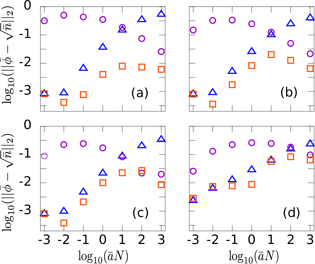
Next, we compare the ground state density distributions of the 1D-NLSEs in different regimes with its 3D-GPE analog. In Fig. 2 we display illustrative examples of the ground state densities obtained for the monomial transverse potentials with $\alpha=4$ and $\alpha\rightarrow\infty$, and anisotropy parameter $\lambda=100$. We observe that for $\bar{a}N=1$ the perturbative and the interpolating profiles are close to that obtained via 3D-GPE, while the TF profile is not so good. Also, by increasing the value of $\bar{a}N$ to $100$, the TF and interpolating profiles approach to the 3D-GPE profile while the perturbative profile departs from it. However, in the intermediate region, $\bar{a}N=10$, only the interpolating profile fits that from the 3D-GPE. We emphasize that this behavior is general, i.e., we observed it for all values tested in the range $\bar{a}N\in[10^{-3},10^{3}]$, $\lambda\in[10,10^{3}]$, and $\alpha\geq 2$. Indeed, in view to make a numerical comparison of the profiles, we display in Fig. 3 the usual $L_{2}$-norm $||\bar{\phi}-\sqrt{\bar{n}}||_{2}=\sqrt{\int(\bar{\phi}-\sqrt{\bar{n}})^{2}d\bar{z}}$ in $\log$ scale, where $\bar{\phi}$ is the ground state for each approximation method and $\bar{n}$ is the 3D-GPE profile. In this figure we used $\lambda=100$ and four different monomial transverse traps ($\alpha=\{2,4,6,\infty\}$). By this figure, in agreement with the visual interpretation of Fig. 2, one can note that the interpolating model presents the lowest values for the $L_{2}$-norm.

Finally, we study the dynamical accuracy of the interpolating model by changing the longitudinal trapping. To this end, we consider the evolution of the ground state of a BEC, previously confined by a longitudinal harmonic potential $V(z)=m\Omega^{2}z^{2}/2$, in a new little tighter harmonic trap, obtained by the replacement $\Omega\to 1.1\Omega$. Indeed, this new trap promotes a pulsation of the condensate axial profile, as one can see in the axial mean width $\langle\bar{z}^{2}\rangle\equiv\int\bar{z}^{2}|\bar{\phi}|^{2}d\bar{z}$ displayed in Fig. 4. Also, by the Fourier analysis of $\langle\bar{z}^{2}\rangle(t)$, we found the principal frequencies and amplitudes of oscillation. Comparisons of these quantities by considering $\alpha=4$ and $\alpha\to\infty$ both with $\lambda=10$ are shown in Fig. 5. Note that, differently from the perturbative and TF models, the frequencies of oscillation $\omega$ and the corresponding amplitudes $A$ of the interpolating model match the 3D-GPE frequencies $\omega_{3D}$ and amplitudes $A_{3D}$, respectively, for all nonlinearity values. We stress that we tested the results shown in Fig. 5 for several values of $\alpha$ and $\lambda$, corroborating the best agreement obtained by the interpolating model as a general feature.

Conclusion. - In this letter we derive effective 1D NLS equations describing the axial effective dynamics of cigar-shaped atomic repulsive Bose-Einstein condensates trapped with anharmonic transverse potentials. In this sense, we implemented a modification on the TF approximation of the transverse chemical potential, which enable us to get accurate estimates to the ground-state profiles, transverse chemical potentials and oscillation patterns. Indeed, by numerical simulations we found that the proposed interpolating model predicts reasonable values even in the crossover regime (between the perturbative and TF regimes), being (to the best of our knowledge) the best 1D model that describes BECs confined by anharmonic transverse potentials. Although we concentrate on the transverse monomial potential, the method may be applied to any monotonic transverse potential for which the TF approximation to $\mu_{\perp}$ is prone to be obtained, offering no additional difficulties.