Andreev reflection assisted lasing in an electromagnetic resonator coupled to a hybrid-quantum-dot

Recent developments in the nanotechnologies have made it feasible to fabricate QDs coupled to a microwave resonator on a chip[1, 2, 3, 4, 5]. Among many theoretical and experimental aspects of the interaction of electromagnetic waves of resonator with QD which have been studied, the possibility of creating lasing in an electromagnetic resonator using QDs has attracted considerable interest.

Different proposals for achieving lasing in electromagnetic resonators coupled to QDs have been considered. Jin et. al[6], liu et. al[7] and Karlewski et.al[8] have shown that in a double-QD connected to metallic leads at finite bias, population inversion can be created by electron tunneling. In Ref.9, Marthaler and his coworkers have shown that lasing without inversion can be achieved by coupling the system to a dissipative environment which enhances the photon emission. Lasing without inversion by coherently driving the system, has recently being considered in Ref.10 for a three-level V-type QD connected to external leads at finite bias. Also, lasing was reported in Ref.11 by coupling the electrons of QD to external periodic driving field. The periodic external field generates Floquet ladder which consist of a series of doublet side-band of dressed-states. The inversion-less gain spectrum in such a system is due to the unequalness of relative populations of doublet dressed-states. Bruhat et.al[12] have also reported optical gain at finite bias in a single-level hybrid-QD[13, 14, 15, 16, 17, 18, 19, 20, 21, 22, 23, 24, 25] which consists of a QD coupled to a normal metal and a superconducting electrode. They showed that if the coupling of the QD to the superconducting electrode is weak enough to suppress the Andreev reflections and widening the width of the density of states at the two edges of the superconducting gap, optical gain can be achieved.

In this work, we consider a single mode electromagnetic resonator coupled to a two-level hQD where the coupling between the superconducting electrode and the QD is not weak. The new features arising in this hybrid system, due to interplay of the fundamental electronic interactions and the proximity effects, are the formation of resonant Andreev reflections and their Flouquet side-resonances and the possibility of sub-gap transport. We show that at appropriate gate voltages and the damping factor of the resonator and above a threshold bias voltage, the Andreev resonances and their Floquet side-resonances in the sub-gap have unequal populations and lasing can be achieved in the frequency range of superconducting gap.

Using the formalism of non-equilibrium Green’s functions at zero temperature, we, at first, determine numerically the linear gain spectrum of the two-level hQD as a function of frequency and gate voltage for a fixed bias voltage. Then, by solving numerically the semi-classical laser equations self-consistently, we determine the lasing regimes, the time-averaged and time-dependent currents through hQD and the photon populations in the resonator in terms of d.c applied bias and gate voltages for two different configurations of the energy levels of the QD and damping factors of the resonator.

This paper is organized as follows. In Sec.II, we introduce our model Hamiltonian and derive the related non-equilibrium Green’s functions for a two-level hQD coupled to a single mode electromagnetic resonator. In Sec.III, we give the necessary relevant formulas for various physical quantities such as average photon number, electron occupations, current through hQD and etc. . Finally, we present our numerical results and conclusions in Sec.IV.

Figure 1 shows a schematic view of our model. We consider a two-level quantum dot dipole coupled to the electric field of a single mode electromagnetic resonator. The two levels of the QD, which we assume to have different parities, are coupled to two electrodes, a superconducting and a normal metal. Therefore, the total Hamiltonian of our model, $H_{M}$, is described by the sum of the following terms:

	$\displaystyle H_{QD}=$	$\displaystyle\underset{n=1,2}{\sum}\,\underset{\sigma=\uparrow,\downarrow}{\sum}\left(\varepsilon_{d,n}+v_{g}\right)\,d_{n,\sigma}^{\dagger}d_{n,\sigma},$		(1)
	$\displaystyle H_{leads}=$	$\displaystyle\underset{k,\sigma}{\sum}\left(\varepsilon_{k}+\mu_{N}\right)\,c_{k,\sigma}^{\dagger}c_{k,\sigma}$
		$\displaystyle+\underset{k,\sigma}{\sum}\left(\tilde{\varepsilon}_{k}+\mu_{S}\right)\,f_{k,\sigma}^{\dagger}f_{k,\sigma}$
		$\displaystyle+\underset{k}{\sum}\Delta\left(f_{k,\uparrow}^{\dagger}f_{-k,\downarrow}^{\dagger}+h.c.\right),$		(2)
	$\displaystyle H_{T}=$	$\displaystyle\underset{k,n,\sigma}{\sum}t_{N}\,\left(c_{k,\sigma}^{\dagger}d_{n,\sigma}+h.c.\right)+t_{S}\,\left(f_{k,\sigma}^{\dagger}d_{n,\sigma}+h.c.\right),$		(3)
	$\displaystyle H_{ph}=\hbar$	$\displaystyle\omega_{0}\left(a^{\dagger}a+\frac{1}{2}\right)$		(4)

and

$$\displaystyle H_{int}=-\underset{\sigma}{\sum}\lambda\left(a+a^{\dagger}\right)\left(d_{1,\sigma}^{\dagger}d_{2,\sigma}+h.c.\right),$$

(5)

where, $H_{QD}$ is the Hamiltonian of isolated two-level QD, $H_{leads}$ is the sum of Hamiltonians of normal and superconducting leads, $H_{T}$ is the tunnelings Hamiltonian of the QD with the electrodes, $H_{ph}$ is the Hamiltonian of single mode electromagnetic resonator and $H_{int}$ is the interaction Hamiltonian of the electric field of resonator with the electric dipole moment of the QD.

In Eqs.(1-3), $d_{n,\sigma}^{\dagger}(d_{n,\sigma}),$ $c_{k,\sigma}^{\dagger}(c_{k,\sigma})$ and $f_{k,\sigma}^{\dagger}(f_{k,\sigma})$ are, respectively, the fermionic creation(annihilation) operators with spin $\sigma$ of QD, normal metal lead and superconducting lead, $\varepsilon_{d,n}$, $n=1,2$, $\tilde{\varepsilon}_{k}$ and $\varepsilon_{k}$ are the orbital energies, $v_{g}=\tilde{v}_{g}+(\mu_{N}+\mu_{S})/2$, $\tilde{v}_{g}$ is the external gate voltage applied to the QD, $\mu_{N}$ and $\mu_{S}$ are the chemical potentials of normal and superconducting leads, $\Delta$ is the superconducting order parameter and $t_{N}$ and $t_{S}$ are the hybridization constants between the QD and the normal and superconducting leads. In Eqs. (4) and (5), $a^{\dagger}(a)$ is the photon creation(annihilation) operator, $\omega_{0}$ is the frequency of the resonator and $\lambda$ is the electric dipole coupling strength of QD and the photon of the resonator.

We determine the possibility of lasing in the resonator of our model, using the semi-classical laser equations[26]. The Heisenberg equation of motion in the mean-field approximation for the mean value of the annihilation operator of the photon is

$$i\hbar\frac{d}{dt}\left\langle a_{H}(t)\right\rangle=\hbar\omega_{0}\left\langle a_{H}(t)\right\rangle-\lambda\underset{\sigma}{\sum}\left\langle\left(d_{H1,\sigma}^{\dagger}(t)d_{H2,\sigma}(t)+h.c.\right)\right\rangle,$$

(6)

where all the operators are in the Heisenberg representation. The semi-classical laser equations can be deduced from the above equation by adding a phenomenological damping term, $-i\hbar\gamma\left\langle a_{H}(t)\right\rangle$, to mimic the resonator’s losses and separating the fast and slow parts of the averaged quantities, using the slowly varying amplitude and phase approximation[26], where the mean values are represented in the following forms

$$\left\langle a_{H}(t)\right\rangle=A_{\bar{\omega}}(t)e^{-i\phi(t)}e^{-i\bar{\omega}t}$$

(7)

and

$$\underset{\sigma}{\sum}\left\langle\left(d_{H1,\sigma}^{\dagger}(t)d_{H2,\sigma}(t)+h.c.\right)\right\rangle=P_{\bar{\omega}}(t)e^{-i\phi(t)}e^{-i\bar{\omega}t}.$$

(8)

In the above equations, $e^{-i\bar{\omega}t}$ is the fast oscillating part, $A_{\bar{\omega}}(t)e^{-i\phi(t)}$ and $P_{\bar{\omega}}(t)e^{-i\phi(t)}$ are the slowly varying parts. Substituting expressions (7) and (8) int Eq. (6) and separating its real and imaginary parts, we obtain

$$\frac{d}{dt}A_{\bar{\omega}}(t)=-\gamma A_{\bar{\omega}}(t)-\frac{\lambda}{\hbar}Im[P_{\bar{\omega}}(t)]$$

(9)

and

$$\frac{d}{dt}\phi(t)=\hbar(\omega_{0}-\bar{\omega})-\lambda\frac{Re[P_{\bar{\omega}}(t)]}{A_{\bar{\omega}}(t)}.$$

(10)

The above equations are the semi-classical laser equations. Their stationary solutions, i.e $\frac{d}{dt}A_{\bar{\omega}}(t)$ and $\frac{d}{dt}\phi(t)$ equal to zero, which must be obtained self consistently with $P_{\bar{\omega}}$, gives the laser threshold, the field intensity or the average photon population and the frequency pulling of the resonator[26].

To determine the steady-state solutions of Eqs. (9) and (10), we compute the $P_{\bar{\omega}}$ and the other relevant physical quantities of hQD by employing the non-equilibrium Green’s functions method. The usage of the non-equilibrium Green’s functions method allows us to take into account the effect of the electrodes on the QD to infinite order of tunneling processes between the QD and the electrodes. This offers an advantage over the conventional quantum master equation method[27, 28], in which the coupling of the electrodes with the QD is treated to the first order processes (weak coupling) or at most the next-to-the-leading order tunneling processes. Furthermore, we use the exact form of the interaction Hamiltonian of the electric field of the resonator with the electric-dipole moment of the QD, which is more accurate and convenient for numerical calculations than the usual dipole Hamiltonian in the rotating wave approximation.

Within the mean-field approximation for the electric field in the resonator, the interaction part of Hamiltonian reduces to

$$\displaystyle\tilde{H}_{int}(t)=\underset{\sigma}{-\lambda\sum}2A_{\bar{\omega}}cos(\bar{\omega}t)\left(d_{1,\sigma}^{\dagger}d_{2,\sigma}+h.c.\right).$$

(11)

We study the case that the superconducting lead is grounded and an static external bias voltage of $V_{b}$ is applied to the normal lead. Furthermore, we work in units where $\hbar=e=c=1$. It is evident that the explicit time dependence of the total Hamiltonian is only through $\tilde{H}_{int}\left(t\right)$ which has a harmonic time dependence with period $\frac{2\pi}{\bar{\omega}}$. So, it is convenient to use Floquet representation

$$\mathcal{F}\left(t,t^{\prime}\right)=\mathrel{{\mathop{\sum}\limits}}\int_{-\frac{\bar{\omega}}{2}}^{\frac{\bar{\omega}}{2}}\frac{d\omega}{2\pi}e^{-i\left(\omega+m\bar{\omega}\right)t}e^{i\left(\omega+n\bar{\omega}\right)t^{\prime}}\mathcal{F}_{mn}\left(\omega\right),$$

(12)

for calculating different Green’s functions and self-energies of the system.

Using Nambu representation, $\Psi^{\dagger}=\left(d_{1,\uparrow}^{\dagger},d_{1,\downarrow},d_{2,\uparrow}^{\dagger},d_{2,\downarrow}\right)$, the Fourier transform of the non-interacting retarded Green’s function, $\left[g^{R}\left(t,t^{\prime}\right)\right]\equiv-i\theta\left(t-t^{\prime}\right)\left\langle\left\{\Psi\left(t\right),\Psi^{\dagger}\left(t^{\prime}\right)\right\}\right\rangle_{0}$, is given by[13, 29]

$$\left[g_{mn}^{R}\left(\omega\right)\right]=\delta_{mn}\left[\left(\omega_{m}+i\eta\right)\left[I\right]-\left[h_{d}\right]-\left[\Sigma_{mn}^{R}\left(\omega_{m}\right)\right]\right]^{-1},$$

(13)

where $\delta_{mn}$ is the Kronecker delta, $\omega_{m}=\omega+m\bar{\omega}$, $\eta$ is an infinitesimal positive constant and $\left[h_{d}\right]$ is a $4\times 4$ diagonal matrix with diagonal elements $\left(\varepsilon_{d,1}+v_{g},-\varepsilon_{d,1}-v_{g},\varepsilon_{d,2}+v_{g},-\varepsilon_{d,2}-v_{g}\right)$. In the sequel the quantities in the brackets represent $4\times 4$ matrices in the Nambu space. Furthermore, the effect of two electrodes on QD is expressed by the self-energies of leads, $\left[\Sigma_{mn}^{R}\left(\omega\right)\right]=\left[\Sigma_{S,mn}^{R}\left(\omega\right)\right]+\left[\Sigma_{N,mn}^{R}\left(\omega\right)\right]$ which are[30]

$$\left[\Sigma_{S,mn}^{R}\left(\omega\right)\right]=\delta_{mn}\left(\begin{array}[]{cccc}a&b&a&b\\ b&a&b&a\\ a&b&a&b\\ b&a&b&a\end{array}\right)$$

(14)

and

$$\left[\Sigma_{N,mn}^{R}\left(\omega\right)\right]=-\delta_{mn}i\Gamma_{N}\left(\begin{array}[]{cccc}1&0&1&0\\ 0&1&0&1\\ 1&0&1&0\\ 0&1&0&1\end{array}\right),$$

(15)

where $a=-i\Gamma_{S}\beta\left(\omega\right)$ and $b=i\Gamma_{S}\beta\left(\omega\right)\frac{\Delta}{\omega}$. The parameter $\beta\left(\omega\right)$ which is related to the normalized BCS density of states is given by $\beta\left(\omega\right)=\frac{\left|\omega\right|}{\sqrt{\omega^{2}-\Delta^{2}}}\theta\left(\left|\omega\right|-\Delta\right)-i\frac{\omega}{\sqrt{\Delta^{2}-\omega^{2}}}\theta\left(\Delta-\left|\omega\right|\right)$. We use the wide-band approximation where the hybridization of QD orbitals with electrodes take the simple form $\Gamma_{N,S}\equiv\pi|t_{N,S}|^{2}\rho_{0}^{N,S}$ where $\rho_{0}^{N}$ and $\rho_{0}^{S}$ are the frequency independent density of states of the normal lead and the normal state of the SC lead, respectively.

We use the Dyson equation in the Floquet basis

$$\left[G_{mn}^{R}\left(\omega\right)\right]=\left[g_{mn}^{R}\left(\omega\right)\right]+\underset{lr}{\sum}\left[g_{ml}^{R}\left(\omega\right)\right]\left[\Pi_{lr}^{R}\left(\omega\right)\right]\left[G_{rn}^{R}\left(\omega\right)\right],$$

(16)

to obtain the interacting retarded Green’s function, $\left[G_{mn}^{R}\left(\omega\right)\right]$, of the QD. The $\left[\Pi_{lr}^{R}\left(\omega\right)\right]$ in the Dyson equation is the retarded self-energy, due to the interaction term of the Hamiltonian, which has the form

$$\left[\Pi_{lr}^{R}\left(\omega\right)\right]=-\lambda A\left(\delta_{l,r+1}+\delta_{l,r-1}\right)\left(\begin{array}[]{cccc}0&0&1&0\\ 0&0&0&-1\\ 1&0&0&0\\ 0&-1&0&0\end{array}\right).$$

(17)

Next, we need to calculate the lesser Green’s function $G^{<}\left(t,t^{\prime}\right)\equiv i\left\langle\Psi^{\dagger}\left(t^{\prime}\right)\Psi\left(t\right)\right\rangle$. We use Keldysh relation for lesser Green’s function which in the Floquet basis is

$$\left[G_{mn}^{<}\left(\omega\right)\right]=\underset{lr}{\sum}\left[G_{ml}^{R}\left(\omega\right)\right]\left[\Sigma_{lr}^{<}\left(\omega\right)\right]\left[G_{rn}^{A}\left(\omega\right)\right].$$

(18)

Here, $\left[G_{rn}^{A}\left(\omega\right)\right]$ is the advanced Green’s function given by $\left[G_{rn}^{A}\left(\omega\right)\right]=\left[G_{rn}^{R}\left(\omega\right)\right]^{\dagger}$, and $\left[\Sigma_{mn}^{<}\left(\omega\right)\right]=\left[\Sigma_{S,mn}^{<}\left(\omega\right)\right]+\left[\Sigma_{N,mn}^{<}\left(\omega\right)\right]$ is the lesser self-energy due to the coupling of QD to the electrodes where

$$\left[\Sigma_{S,mn}^{<}\left(\omega\right)\right]=\left[\left[\Sigma_{S,mn}^{A}\left(\omega\right)\right]-\left[\Sigma_{S,mn}^{R}\left(\omega\right)\right]\right]f\left(\omega\right)$$

(19)

and

$$\left[\Sigma_{N,mn}^{<}\left(\omega\right)\right]=\delta_{mn}2i\Gamma_{N}\left(\begin{array}[]{cccc}f^{+}\left(\omega\right)&0&f^{+}\left(\omega\right)&0\\ 0&f^{-}\left(\omega\right)&0&f^{-}\left(\omega\right)\\ f^{+}\left(\omega\right)&0&f^{+}\left(\omega\right)&0\\ 0&f^{-}\left(\omega\right)&0&f^{-}\left(\omega\right)\end{array}\right),$$

(20)

with $f\left(\omega\right)=\theta\left(-\omega\right)$ and $f^{\pm}\left(\omega\right)=\theta\left(V_{b}\mp\omega\right)$, which are the Fermi-Dirac distribution functions for the superconducting and normal metal leads at zero temperature.

We now, present the various relevant physical quantities related to our model system using different Green’s functions. The first quantities of interest are the average polarization $\left\langle P\left(t\right)\right\rangle=\underset{\sigma}{\sum}\left\langle\left(d_{H1,\sigma}^{\dagger}(t)d_{H2,\sigma}(t)+h.c.\right)\right\rangle$ which is related to the lesser Green’s function and the linear optical susceptibility

$$\chi_{e}^{r}\left(t-t^{\prime}\right)=-i\theta\left(t-t^{\prime}\right)\left\langle\left[P(t^{\prime}),P(t)\right]\right\rangle_{o},$$

(21)

where $\left\langle...\right\rangle_{o}$ indicates expectation-value with respect to the non-interacting ground-state of the hQD. Using the definition of the lesser Green’s function, we get

$$\displaystyle\left\langle P\left(t\right)\right\rangle=-i\left[G^{<}(t,t)\right]_{13+31-24-42}$$

(22)

or

$$\left\langle P\left(t\right)\right\rangle=-i\underset{m,n}{\sum}\int_{-\frac{\bar{\omega}}{2}}^{\frac{\bar{\omega}}{2}}\frac{d\omega}{2\pi}e^{-i(m-n)\bar{\omega}t}\left[G_{mn}^{<}\left(\omega\right)\right]_{13+31-24-42},$$

(23)

where the subscripts outside brackets represent different matrix elements in the Nambu space which must be summed up. Setting the constant phase, $\phi$, to zero and using Eq.(8), we obtain for the steady-state amplitude of the polarization and the linear optical susceptibility

$$P_{\bar{\omega}}=-i\underset{m}{\sum}\int_{-\frac{\bar{\omega}}{2}}^{\frac{\bar{\omega}}{2}}\frac{d\omega}{2\pi}\left[G_{m+1,m}^{<}\left(\omega\right)\right]_{13+31-24-42},$$

(24)

and[31]

	$\displaystyle\chi_{e}^{r}\left(\omega\right)=($	$\displaystyle\boldsymbol{F}_{33}^{11}\left(\omega\right)+\boldsymbol{F}_{13}^{13}\left(\omega\right)-\boldsymbol{F}_{23}^{14}\left(\omega\right)-\boldsymbol{F}_{43}^{12}\left(\omega\right)+$
		$\displaystyle\boldsymbol{F}_{11}^{33}\left(\omega\right)+\boldsymbol{F}_{31}^{31}\left(\omega\right)-\boldsymbol{F}_{41}^{32}\left(\omega\right)-\boldsymbol{F}_{21}^{34}\left(\omega\right)+$
		$\displaystyle\boldsymbol{F}_{44}^{22}\left(\omega\right)+\boldsymbol{F}_{24}^{24}\left(\omega\right)-\boldsymbol{F}_{34}^{21}\left(\omega\right)-\boldsymbol{F}_{14}^{23}\left(\omega\right)+$
		$\displaystyle\boldsymbol{F}_{22}^{44}\left(\omega\right)+\boldsymbol{F}_{42}^{42}\left(\omega\right)-\boldsymbol{F}_{12}^{43}\left(\omega\right)-\boldsymbol{F}_{32}^{41}\left(\omega\right)),$		(25)

where

$$\boldsymbol{F}_{pq}^{mn}\left(\omega\right)\equiv-i\underset{l}{\sum}\int\frac{d\omega^{\prime}}{2\pi}\{\left[G_{0l}^{R}\left(\omega+\omega^{\prime}\right)\right]_{mn}\left[G_{l0}^{<}\left(\omega^{\prime}\right)\right]_{pq}+\left[G_{0l}^{<}\left(\omega+\omega^{\prime}\right)\right]_{mn}\left[G_{l0}^{A}\left(\omega^{\prime}\right)\right]_{pq}\}.$$

(26)

Furthermore, the time-averaged expectation-value of the electron and hole occupations of each orbital could be calculated using

$$\left\langle n_{d,m}\left(t\right)\right\rangle_{t}=-2i\underset{l}{\sum}\int_{-\frac{\bar{\omega}}{2}}^{\frac{\bar{\omega}}{2}}\frac{d\omega}{2\pi}\left[G_{ll}^{<}\left(\omega\right)\right]_{mm}\left(\omega\right),\>m=1,..,4$$

(27)

where $\left\langle...\right\rangle_{t}$ means time-averaged expectation value, $m=1,2$ and $m=3,4$ designate, respectively, the electron and hole states of the first and second levels of QD and the factor two is due to the electron’s spin. Moreover, the time-averaged total density of states(DOS) of the QD could be obtained from retarded Green’s function as

$$\rho\left(\omega\right)=-\frac{1}{\pi}Tr\left[Im\left[G_{00}^{R}\left(\omega\right)\right]\right].$$

(28)

where $Tr\left[...\right]$ represents trace with respect to the Nambu indeices. Finally, for calculating the time-dependent and time-averaged electric current through the QD in terms of the Green’s functions and the self-energies in Floquet representations, we use the following expressions[13, 32];

	$\displaystyle I(t)=\underset{l,m,n}{\sum}\int_{-\frac{\bar{\omega}}{2}}^{\frac{\bar{\omega}}{2}}\frac{d\omega}{2\pi}e^{-i(l-n)\bar{\omega}t}[$	$\displaystyle\left[G_{lm}^{R}\left(\omega\right)\right]\left[\Sigma_{N,mn}^{<}\left(\omega\right)\right]+\left[G_{lm}^{<}\left(\omega\right)\right]\left[\Sigma_{N,mn}^{A}\left(\omega\right)\right]$
		$\displaystyle-\left[\Sigma_{N,lm}^{<}\left(\omega\right)\right]\left[G_{mn}^{A}\left(\omega\right)\right]-\left[\Sigma_{N,lm}^{R}\left(\omega\right)\right]\left[G_{mn}^{<}\left(\omega\right)\right]]_{11-22+33-44}.$		(29)

and

	$\displaystyle\left\langle I\left(t\right)\right\rangle_{t}=\underset{l,m}{\sum}\int_{-\frac{\bar{\omega}}{2}}^{\frac{\bar{\omega}}{2}}\frac{d\omega}{2\pi}[$	$\displaystyle\left[G_{lm}^{R}\left(\omega\right)\right]\left[\Sigma_{N,ml}^{<}\left(\omega\right)\right]+\left[G_{lm}^{<}\left(\omega\right)\right]\left[\Sigma_{N,ml}^{A}\left(\omega\right)\right]$
		$\displaystyle-\left[\Sigma_{N,lm}^{<}\left(\omega\right)\right]\left[G_{ml}^{A}\left(\omega\right)\right]-\left[\Sigma_{N,lm}^{R}\left(\omega\right)\right]\left[G_{ml}^{<}\left(\omega\right)\right]]_{11-22+33-44}.$		(30)

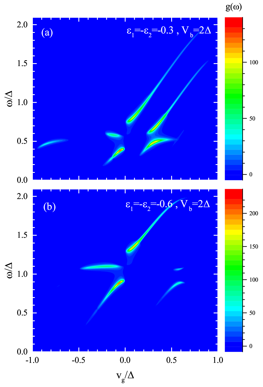
In the preceding sections, the necessary formulas for determining the lasing conditions for the hQD-resonator system were presented. We now investigate the prospect of lasing in such a system. We start by calculating, at first, the linear gain spectra, $g(\omega)=-4\pi\omega Im\left[\chi_{e}^{r}\left(\omega\right)\right]$, of the QD which can be obtained from the imaginary part of the linear optical susceptibility, given by Eq.(25). We consider the following two different energy configurations for the two levels of QD; $\varepsilon_{d,1}=-\varepsilon_{d,2}=-0.3\Delta$ and $\varepsilon_{d,1}=-\varepsilon_{d,2}=-0.6\Delta$. The results as functions of $\omega/\Delta$ and $v_{g}$ for $\mu_{S}$ equal to zero, $\mu_{N}=V_{b}=2\Delta$, $\Gamma_{S}=0.1\Delta$ and $\Gamma_{N}=0.01\Delta$, are depicted in Figs.2 (a) and (b). Although one might expect to see non-zero gain only at frequencies equal to the energy difference of the two levels of the QD but, as we see in Fig.2, this does not happen in our model system. Instead, we see different regions for non-zero gain which are dependent on the parameters of the QD. The origin of these gain regions is due to the fact that it is, essentially, the electron transitions between different resonant Andreev reflections in the sub-gap regions which are responsible for the non-zero gain in the system. In Figs.2 (a) and (b), in the first case, the maximum gain occurs at frequency $\omega=0.38\Delta$ and gate voltage $v_{g}=-0.06\Delta$ and in the second case, the maximum gain is at $\omega=0.87\Delta$ and $v_{g}=-0.05\Delta$.

In order to clarify the above discussion about the origin of the non-zero gain in the system, we present in Figs.3 (a) and (b), the density of states of QD and their relative populations for the two aforementioned cases and compare them with the situations when the gate voltages are zero. The four resonances in the density of states are due to the Andreev reflections. It can be seen from Figs. 3 (a) and (b) that the relative populations of the Andreev resonances are dependent on the applied external bias and gate voltages and they could have some population inversions in the sub-gap energies in some specific configurations. The maximum linear gains in Fig.2(a) and (b) are due to the transitions from C to B resonances, depicted in Fig.3(a) and (b), respectively.

We next consider the possibility of lasing in a system of a single mode electromagnetic resonator coupled to a hQD. We choose the aforementioned configurations for hQD and two different damping factors; $\gamma=10^{-3}\Delta$ and $\gamma=10^{-4}\Delta$ for the resonator. We solve the semi-classical laser Eqs.(9) and (10) with Eq.(24) for the polarization of hQD numerically and self-consistently.

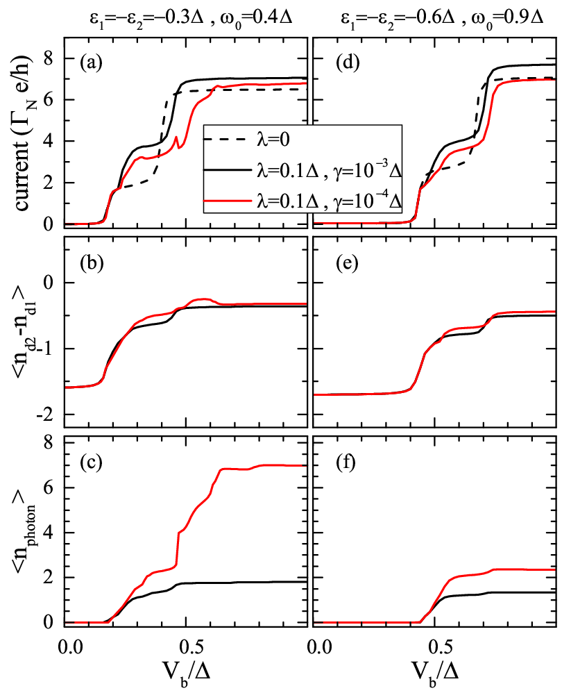
In Fig.4, we have depicted the time-averaged current through the QD, the average population differences of the two levels of QD, and the average photon populations in the resonator as functions of external applied bias for coupling constant $\lambda=0.1\Delta$. In Figs.4(a)-(c), the frequency of the resonator is $\omega_{0}=0.4\Delta$ and in Figs4(d)-(e), $\omega_{0}=0.9\Delta$. Depending on the ratio of the intensity of electric field in the resonator to the frequency of resonator and the magnitude of applied bias voltage, we observe two regimes of lasing for both cases. For $\gamma=10^{-3}\Delta$, we obtain small values of the aforementioned ratio and the stimulated emission is solely between the Andreev resonances and lasing occurs above a threshold bias voltage. When we reduce the damping factor of the resonator to $\gamma=10^{-4}\Delta$, the ratio of the intensity of the electric field in the resonator to the frequency of the resonator becomes large and the Floquet-Andreev side-resonances, with frequencies obeying relation; $\omega_{m}=\omega_{A}+m\bar{\omega},m=0,\pm 1,...,$ where $\omega_{A}$’s are the frequencies of Andreev resonances, acquire sizable amplitudes in the superconducting gap, and above certain threshold bias voltage, their populations and frequency differences are such that they can participate in the stimulated emission in two different ways; either in a cascaded manner which results in a sudden increase of the average number of photons in the resonator without appreciable change in the time-averaged current through the QD, see Figs.4(a) and (c), or through extra electron transitions between the Floquet-Andreev side-resonances which we observe in Figs4(d) and (f). In the latter case, the increase in the average number of photons in the resonator is accompanied with an increase in the time-averaged current through the QD. Furthermore, the on-set of lasing in the resonator is accompanied by the appearance of oscillating polarization current through the hQD which is depicted in Fig.5.

In conclusion, we numerically investigated the possibility of lasing in a single mode electromagnetic resonator coupled to a two-level hQD when driven out of equilibrium by applying external bias voltages. It is found that at specific gate voltages and above certain threshold bias voltages the two-level QD connected to a normal metal and a superconducting electrodes has non-zero gain spectrum due to the resonant Andreev reflections and when coupled to an electromagnetic resonator, for damping factors of the resonator below certain thresholds, Andreev-Floquet side-resonances also appear in the sub-gap regions and lasing can happens in two different regimes. In addition, with the on-set of lasing in the resonator, the current through hQD beside its d.c. (time-averaged) component, acquires an oscillating part. Thus, by monitoring the d.c. and a.c. components of the current through the hQD, the on-set of lasing and its regime can, in principle, be identified.

References

- [1] MR Delbecq, Vivien Schmitt, FD Parmentier, Nicolas Roch, JJ Viennot, Gwendal Fève, Benjamin Huard, Christophe Mora, Audrey Cottet, and Takis Kontos. Coupling a quantum dot, fermionic leads, and a microwave cavity on a chip. Physical Review Letters, 107(25):256804, 2011.
- [2] C. Roy and S. Hughes. Influence of electron–acoustic-phonon scattering on intensity power broadening in a coherently driven quantum-dot–cavity system. Phys. Rev. X, 1:021009, Nov 2011.
- [3] T Frey, PJ Leek, M Beck, Alexandre Blais, Thomas Ihn, Klaus Ensslin, and Andreas Wallraff. Dipole coupling of a double quantum dot to a microwave resonator. Physical Review Letters, 108(4):046807, 2012.
- [4] C. Bergenfeldt and P. Samuelsson. Microwave quantum optics and electron transport through a metallic dot strongly coupled to a transmission line cavity. Phys. Rev. B, 85:045446, Jan 2012.
- [5] Marco Schiró and Karyn Le Hur. Tunable hybrid quantum electrodynamics from nonlinear electron transport. Phys. Rev. B, 89:195127, May 2014.
- [6] Pei-Qing Jin, Michael Marthaler, Jared H Cole, Alexander Shnirman, and Gerd Schön. Lasing and transport in a quantum-dot resonator circuit. Physical Review B, 84(3):035322, 2011.
- [7] Y-Y Liu, J Stehlik, Christopher Eichler, MJ Gullans, Jacob M Taylor, and JR Petta. Semiconductor double quantum dot micromaser. Science, 347(6219):285–287, 2015.
- [8] Christian Karlewski, Andreas Heimes, and Gerd Schön. Lasing and transport in a multilevel double quantum dot system coupled to a microwave oscillator. Physical Review B, 93(4):045314, 2016.
- [9] Michael Marthaler, Y Utsumi, Dmitri S Golubev, Alexander Shnirman, and Gerd Schön. Lasing without inversion in circuit quantum electrodynamics. Physical review letters, 107(9):093901, 2011.
- [10] Luqi Yuan, Da-Wei Wang, Christopher O’Brien, Anatoly A Svidzinsky, and Marlan O Scully. Sideband generation of transient lasing without population inversion. Physical Review A, 90(2):023836, 2014.
- [11] J Stehlik, Y-Y Liu, C Eichler, TR Hartke, X Mi, MJ Gullans, JM Taylor, and JR Petta. Double quantum dot floquet gain medium. Physical Review X, 6(4):041027, 2016.
- [12] LE Bruhat, JJ Viennot, MC Dartiailh, MM Desjardins, Takis Kontos, and Audrey Cottet. Cavity photons as a probe for charge relaxation resistance and photon emission in a quantum dot coupled to normal and superconducting continua. Physical Review X, 6(2):021014, 2016.
- [13] Qing-feng Sun, Jian Wang, and Tsung-han Lin. Resonant andreev reflection in a normal-metal–quantum-dot–superconductor system. Physical Review B, 59(5):3831, 1999.
- [14] Qing-feng Sun, Hong Guo, and Tsung-han Lin. Excess kondo resonance in a quantum dot device with normal and superconducting leads: The physics of andreev-normal co-tunneling. Phys. Rev. Lett., 87:176601, Oct 2001.
- [15] J. C. Cuevas, A. Levy Yeyati, and A. Martín-Rodero. Kondo effect in normal-superconductor quantum dots. Phys. Rev. B, 63:094515, Feb 2001.
- [16] Mariusz Krawiec and Karol I Wysokiński. Electron transport through a strongly interacting quantum dot coupled to a normal metal and bcs superconductor. Superconductor Science and Technology, 17(1):103, 2003.
- [17] Long Bai, Zheng-Zhong Zhang, and Liang Jiang. Andreev reflection current through a molecule quantum dot in the presence of the electron–phonon interaction and the spin-flip scattering. Physics Letters A, 375(3):661–665, 2011.
- [18] Sheng-Nan Zhang, Wei Pei, Tie-Feng Fang, and Qing-feng Sun. Phonon-assisted transport through quantum dots with normal and superconducting leads. Physical Review B, 86(10):104513, 2012.
- [19] R Allub and CR Proetto. Hybrid quantum dot–superconducting systems: Josephson current and kondo effect in the narrow-band limit. Physical Review B, 91(4):045442, 2015.
- [20] I Weymann and KP Wójcik. Andreev transport in a correlated ferromagnet-quantum-dot-superconductor device. Physical Review B, 92(24):245307, 2015.
- [21] Sun-Yong Hwang, David Sánchez, and Rosa López. A hybrid superconducting quantum dot acting as an efficient charge and spin seebeck diode. New Journal of Physics, 18(9):093024, 2016.
- [22] T Nussbaumer, W Belzig, et al. Quantum dot coupled to a normal and a superconducting lead. Nanotechnology, 15(7):S479, 2004.
- [23] RS Deacon, Yoichi Tanaka, A Oiwa, R Sakano, K Yoshida, K Shibata, K Hirakawa, and S Tarucha. Tunneling spectroscopy of andreev energy levels in a quantum dot coupled to a superconductor. Physical review letters, 104(7):076805, 2010.
- [24] R. S. Deacon, Y. Tanaka, A. Oiwa, R. Sakano, K. Yoshida, K. Shibata, K. Hirakawa, and S. Tarucha. Kondo-enhanced andreev transport in single self-assembled inas quantum dots contacted with normal and superconducting leads. Phys. Rev. B, 81:121308, Mar 2010.
- [25] Travis Dirks, Taylor L Hughes, Siddhartha Lal, Bruno Uchoa, Yung-Fu Chen, Cesar Chialvo, Paul M Goldbart, and Nadya Mason. Transport through andreev bound states in a graphene quantum dot. Nature Physics, 7(5):386–390, 2011.
- [26] Hermann Haken. Laser theory. Springer Science & Business Media, 2012.
- [27] Christian Ginzel, Hans-Jürgen Briegel, Ullrich Martini, Berthold-Georg Englert, and Axel Schenzle. Quantum optical master equations: The one-atom laser. Physical Review A, 48(1):732, 1993.
- [28] Jürgen König, Herbert Schoeller, and Gerd Schön. Zero-bias anomalies and boson-assisted tunneling through quantum dots. Physical review letters, 76(10):1715, 1996.
- [29] Qing-feng Sun, Jian Wang, and Tsung-han Lin. Photon-assisted andreev tunneling through a mesoscopic hybrid system. Physical Review B, 59(20):13126, 1999.
- [30] Piotr Trocha and Józef Barnaś. Spin-polarized andreev transport influenced by coulomb repulsion through a two-quantum-dot system. Physical Review B, 89(24):245418, 2014.
- [31] Hartmut Haug and Antti-Pekka Jauho. Quantum kinetics in transport and optics of semiconductors, volume 2. Springer, 2008.
- [32] Jian Wang, Baigeng Wang, Wei Ren, and Hong Guo. Conservation of spin current: Model including self-consistent spin-spin interaction. Physical Review B, 74(15):155307, 2006.