Distance, reddening and three dimensional structure of the SMC : Using RRab stars
Abstract
We present a study of simultaneous determination of mean distance and reddening to the Small Magellanic Cloud (SMC) using the two photometric band RR Lyrae data. Currently available largest number of highly accurate and precise light curve data of the fundamental mode RR Lyrae stars (RRab) with better areal coverage released by the Optical Gravitational Lensing Experiment (OGLE)-IV project observed in the two photometric bands were utilised simultaneously in order to determine true distance and reddening independently for each of the individual RRab stars. Different empirical and theoretical calibrations leading to the determination of absolute magnitudes of RRab stars in the two bands, and along with their mean magnitudes were utilised to calculate the apparent distance moduli of each of these RRab stars in these two bands. Decomposing the apparent distance moduli into true distance modulus and reddening in each of these two bands, individual RRab distance and reddening were estimated solving the two apparent distance moduli equations. Modeling the observed distributions of the true distance moduli and reddenings of the SMC RRab stars as Gaussian, the true mean distance modulus and mean reddening value to the SMC were found to be mag and mag, respectively. This corresponds to a distance of kpc to the SMC. The three dimensional distribution of the SMC RRab stars was approximated as ellipsoid. Then using the principal axes transformation method (Deb & Singh, 2014) we find the axes ratios of the SMC: with and . These results are in agreement with other recent independent previous studies using different tracers and methodologies.
Keywords:
stars: variables: RR Lyrae-stars:fundamental parameters - stars: Population II - galaxies: statistics - galaxies:structure - galaxies:Magellanic Clouds1 Introduction
Studies of variable stars are crucial for addressing several key astrophysical problems and issues. For example, distance determination is one of the most difficult but essential ingredients in modern astronomy. The pulsating stars such as Cepheids and RR Lyraes play pivotal roles in the definition of the distance ladder. RR Lyrae stars provide a very useful means to obtain highly precise ( error) distance measurements in the range kpc. They can be used to anchor Galactic and extra-galactic distances, to constrain the value of value of the Hubble constant upto accuracy and to study the galactic structures (Deb & Singh, 2014; Deb et al., 2015; Beaton et al., 2016). Furthermore using the light curves of these stars, it is also possible to determine their various physical and chemical parameters including the reddening towards the line of sight (Deb & Singh, 2010; Wagner-Kaiser & Sarajedini, 2017). The population II distance scale relies on the absolute magnitudes of the RR Lyraes which in turn depend on the information about metallicity. Using RR Lyraes found in globular clusters, an estimate of the age of the cluster and hence a lower bound on the age of the Universe can be determined. Several empirical and theoretical relations connecting the metallicity and absolute magnitudes for RR Lyrae stars available in multiwavelength bands provide the robust means of obtaining much improved distances and reddening estimations (Bono et al., 2003; Catelan et al., 2004; Del Principe et al., 2005; Marconi et al., 2015).
Recently there has been a lot of interest in building a distance ladder based on Pop II stars such as RR Lyrae stars because of numerous advantages of these old stellar population and tracers of low-mass stars, against the Pop I stars such as Cepheids. For instance, their presence in all kinds of galaxies as well in low density stellar haloes which have low reddening and relatively uniform and low metallicity populations make them robust and excellent standard candles independent of Cepheids. They are also much more numerous than the Population II or Type II Cepheids (Beaton et al., 2016).
The SMC is a dwarf irregular galaxy connected by a hydrogen gas and stellar bridge to the Large Magellanic Cloud (LMC). Being the satellite galaxies of the Milky Way, they are useful for calibrations for many standard candles (Graczyk et al., 2014). A large number of studies involving the distance, reddening and three dimensional structure of the SMC rely on the available existing light curve data of variable stars generated from various astronomy missions and all sky surveys. Our present knowledge is limited by the flow of available data. During the last few decades, the OGLE project has revolutionized in the collection of a huge number of variable star light curve data of the Galaxy, the SMC and LMC in -bands which was never done ever before. This revolution in collecting data by OGLE has led to the discovery of a number of variable stars in the the Galaxy as well as Magellanic Clouds and also helped to study a particular galaxy from its tracers of various standard candles. A large number of studies were devoted to study the SMC using the OGLE archival data of RR Lyrae stars and produced some significant results in recent decades, viz., Deb & Singh (2010); Kapakos et al. (2011); Haschke et al. (2011); Haschke et al. (2012a); Subramanian & Subramaniam (2012); Deb et al. (2015), to mention a few.
The distance to the SMC is of vital interest to anchor and calibrate the extragalactic distance scale. There exist several studies in the literature which attempt to obtain the distance to the SMC using RRab, Cepheid and eclipsing binary light curve data ranging from optical to near-infrared (NIR) bands (Szewczyk et al., 2009; Inno et al., 2013; Graczyk et al., 2014; Scowcroft et al., 2016, among others). Determinations of mean distance, reddening as well as three dimensional structure of the SMC utilising simultaneous - and -band data of RRab stars from the OGLE-IV database constitute the broader context of the present study. The availability of light curve data of an RRab star observed in two photometric -bands has two major implications: (1) independent distance determination free from the effect of reddening and (2) reddening estimation. This is because the effect due to the reddening in the distance determination can be disentangled from the observed apparent distance modulus by using the light curve data of the same RRab star available in two photometric -bands. Distance determination to the SMC or any other galaxy/globular cluster using RRab stars with single band photometric data require reddening estimations to be taken from other sources of reddening maps such as Burstein & Heiles (1982); Schlegel et al. (1998); Zaritsky et al. (2002) or some other reddening maps. For many targets where the foreground reddening is high and spatially variable, the reddening values can be directly determined from the RRab stars themselves rather than relying on those aforementioned reddening maps if the data are available in two photometric bands.
Although the method developed in the present study has been applied for the RRab stars, it is in general applicable to any periodic variable stars such as Cepheids which act as ‘standard candles’. This method is expected to give as accurate a result in the distance determination as those of the distance determination techniques based on Period-Wesenheit (PW) relations. This is because of the fact that the distance determinations in the present study as well as those based on PW relations are reddening-free by constructions. Despite giving almost the same result of distance determinations, this method is expected to provide an additional advantage over the PW-based methods as it also yields information about the reddening value towards the location of the star apart from finding its distance simultaneously. This information will serve to very useful in the determination of three dimensional structure as well as constructing the reddening map of the host galaxy/globular cluster.
Wesenheit functions are widely used in classical Cepheids to obtain reddening-free PW relations for accurate distance determinations when the data in two photometric bands are available (Madore, 1982; Freedman et al., 2001; Majaess et al., 2011). These relations can also be adopted for RR Lyrae stars (Kovács & Walker, 2001; Di Criscienzo et al., 2004; Majaess, 2010; Majaess et al., 2011; Braga et al., 2015; Marconi et al., 2015, among others). In the case of RR Lyrae stars, the existence of reddening-free PW relations has been firmly supported from the findings of Marconi et al. (2015) and Braga et al. (2015), respectively. Using the PW relations for RR Lyrae stars, Martínez-Vázquez et al. (2015) found the reddening-free distance modulus to the Sculptor dSph, Braga et al. (2015) derived the distance to the globular cluster M4 (NGC 6121), etc., among others. The distance determination using a different method, i.e. the Wesenheit function, which has been largely applied recently, would provide an interesting and independent alternative result to the present analysis.
The main rationale of this paper is to simultaneously exploit the available - and -band OGLE-IV data of more than SMC RRab stars in order to independently determine their distances and reddenings. This information of individual RRab star will be useful to determine the true mean distance, reddening and three dimensional structure of the SMC as well as to construct its reddening map. In an earlier study of the SMC, Deb et al. (2015) used the - and -band RRab light curve data separately from the OGLE-III catalog to study the three dimensional structure and metallicity distribution of the SMC using a very limited number of RRab stars available in the database. Apart from that, the study by Deb et al. (2015) does not use both the - and -band data simultaneously to determine the reddening values but uses the reddening values from the Zaritsky et al. (2002) reddening map.
The paper is organised as follows: Section 2 describes the OGLE-IV RRab data of the SMC and sample selection for the analysis in the present study. The methodologies developed here for the distance determination and reddening estimations are described in Section 3. Metallicity relation of Nemec et al. (2013) was used to derive and values of the sample of RRab stars. Section 4 demonstrates the application of the technique to an RRab star in the OGLE-IV database, while Section 5 describes the comparison of the values of distance and reddening with those obtained using other empirical and theoretical relations. For comparison with the distance obtained in the present study, distances are calculated from reddening-free Wesenheit distance moduli () using the observed and absolute Wesenheit magnitudes. Absolute Wesenheit magnitudes of RRab stars are calculated using the theoretical Period-Wesehnehit-Metallicity (PWZ) relation of Braga et al. (2015). Mean distance and reddening determination of the SMC are discussed in Section 6, whereas Section 7 gives an account of error estimation of the derived quantities. The period-colour relation derived using the independent reddening values in the present study is discussed in Section 8. Determination of the three dimensional structure of the SMC applying different fitting algorithms is discussed in Section 9. Results obtained from the above analyses are compared with those obtained using the Smolec (2005) metallicity relation and with other values available in the literature in Section 10. Lastly, the summary and conclusions of the present investigation are presented in Section 11.

|

|
|---|---|

|

|
2 The Data and Sample Selection
The OGLE-IV is one of the largest sky variability surveys worldwide in recent times which covers over square degrees in the sky and regularly monitors over a billion sources. The main targets of this project include the inner Galactic bulge and the Magellanic system. The photometric accuracy of this project is of the order of mag (Udalski et al., 2015; Soszyński et al., 2016a). The number of new sources in this part of the project has at least doubled as compared to the last OGLE-III project (Udalski et al., 2015). The details of the OGLE-IV project, the instruments such as the telescope, mosaic CCD (Charge Coupled Device) camera and the -filters are provided in Udalski et al. (2015).
The OGLE-IV collection of RRab stars is an extension of OGLE-III catalog to the regions covered by the OGLE-IV fields. The areal coverage of the OGLE-III catalog was square degrees of the sky which covers mostly the central regions of the LMC and SMC. The recently released OGLE-IV catalog covers around square degrees of the sky which include the larger part of the Magellanic system covering the outermost parts as well as the Magellanic Bridge connecting them. The OGLE-IV database contains the data obtained with the -meter Warsaw telescope equipped with a -detector mosaic CCD camera located at Las Campanas Observatory (operated by the Carnegie Institution for Science), Chile. In order to carry out the present study, RRab stars were selected from the OGLE-IV catalog of variable stars that consist of -year of archival data observed between Match and July . The database contains Johnson and Cousins band light curve data, with the majority of the observations obtained in the -band (Soszyński et al., 2016b).
The classification of the SMC RRab stars in the OGLE-IV catalog was based on the periods, amplitudes and Fourier parameters of the light curves obtained from the Fourier cosine decomposition method (Soszyński et al., 2016b). The catalog contains information about the OGLE ID, mean magnitudes of the light curves , in the and -bands, respectively, period , error in the period , time of maximum brightness , amplitude in the -band , Fourier parameters in the -band as well as time-series photometry in the -bands. The OGLE-IV catalog provides new RR Lyrae stars in the LMC and SMC which were not present in the earlier phases of the OGLE survey. This is by far the largest number of RRab light curve data generated with complete phase coverage in the - and -bands obtained in the SMC. The OGLE-III catalog consists of SMC RRab stars with their number increased to in the new data release of OGLE-IV. The -band RRab light curve data of OGLE-IV have even phase coverage containing an average of accurate and precise photometric observations with the exposure time of s. On the other hand, -band light curves of RRab star contain only an average of data points ( of the -band observations) per light curve with the exposure time of s (Soszyński et al., 2016b). Since the database does not provide standard errors in the mean magnitudes as well in the Fourier parameters, we do not use these values for the analysis done in this paper. We use only the light curve data available in both the two bands () along with the information about their periods () and epochs of maximum light ().
The available - and -band photometric light curves of common SMC RRab stars from the OGLE-IV catalog were matched. The matched light curves were further subjected to pre-selection. The -band light curves contain comparatively more number of data points than the corresponding -band light curves. Out of RRab stars available in the catalog, there are RRab stars which have complementary light curve data available in both the - and -band. We have selected only those common light curves which contain at least data points in the -band for reliable light curve parameter estimations. This condition further reduces the number of common RRab stars in both the two bands to for analysis. The light curves of these RRab stars were Fourier decomposed using sinusoidal law to derive their mean apparent magnitudes, amplitudes in the and -band and Fourier parameters for the and -band light curves, respectively. Apparent mean magnitudes and Fourier parameters in the and -band are obtained from the Fourier sine decomposition of the light curves (Deb et al., 2015)
| (1) |
using the seven and fourth order Fourier fits for the and bands, respectively. Here is the mean magnitude, is the angular frequency and is the time of observations. represents the epoch of maximum light. The phased light curves are obtained using
where represents one pulsational cycle of the RRab stars. A collection of four randomly selected sample of RRab stars with thier corresponding OGLE IDs and periods in the and -band is shown in Fig. 1. The corresponding Fourier fits for the respective and -band are also shown in blue and solid colour solid lines. The phase differences and amplitude ratios are evaluated and standard errors are determined following Deb & Singh (2010) for both the and bands, respectively. It should be noted that radian. Since the -band light curves contain more number of data points the Fourier parameters obtained in this band will be more accurate and precise as compared to the corresponding -band Fourier parameters. In this paper we use to denote the Fourier phase parameter in the band obtained from the Fourier sine decomposition. The light curve parameters obtained from the Fourier sine decomposition method as given by equation (1) are listed in Table 1.
A comparison of the light curve parameters of stars in the present study (along abscissa) with those available from the OGLE-IV database Soszyński et al. (2016b) (along ordinate) in shown in Fig. 2 as scatter plots. As shown in the figure (This work) has been calculated by subtracting from (provided in the last column of Table 1) obtained from the Fourier sine decomposition in the present study just for comparison with the value of as given in the database which is obtained from the Fourier cosine decomposition. The sine and cosine phase parameters differ by radians, i.e, (Deb & Singh, 2010; Nemec et al., 2011). If the value of (This work) comes out to be negative, then a value of is added to it so that its value always lies in the interval .
The Fourier phase parameter is often used to determine the metallicity of an RRab star along with the information of the period of an RRab star (Jurcsik & Kovacs, 1996; Smolec, 2005; Nemec et al., 2013, among others). A histogram plot of the distribution of standard errors in is shown in Fig. 3, where . In order to select a clean sample of the SMC RRab stars for the present analysis, we apply the selection criteria based on OGLE-determined periods , the mean magnitudes , observed colours , amplitudes (), error in the -band Fourier phase parameter determined from the Fourier analysis of the light curves as described by equation (1) and metallicities . RRab stars with d, mag, mag, mag, mag, mag, , dex were chosen for the analysis. Here represents the metallicity in the Zinn & West (1984) scale. Most of the selection criteria were adapted from Deb et al. (2015) while a few of them, viz., from Deb & Singh (2010); colour from Haschke et al. (2012a) with slight modifications. Certain selection criteria were always applied in the literature in order to choose a clean sample of RRab stars belonging to a particular galaxy free from any possible contamination due to the foreground objects of any other galaxy (Pejcha & Stanek, 2009; Haschke et al., 2011; Deb et al., 2015). The application of this final selection criteria applied on the RRab stars further reduces their number to for the light curve analysis.

|

|

|
|---|
Availability of a large number of SMC RRab light curve data in OGLE-IV database with complete phase coverage in two different photometric bands with an improved areal coverage provides a unique opportunity to determine the distance and reddening of each of the individual stars. Since the database of RRab stars is substantially larger than any previously studied subset of SMC RRab stars, this wealth of new data can in turn be used to refine our knowledge about the distance scale and reddening distribution to the SMC. This will lead to a detailed understanding of the three dimensional structure, dust and metallicity distribution of the SMC.
| OGLE ID | [days] | [mag] | [mag] | [mag] | [mag] | [rad] |
|---|---|---|---|---|---|---|
| [mag] | [mag] | [mag] | [mag] | [rad] | ||
| OGLE-SMC-RRLYR-0001 | 0.5588145 | 19.067 | 19.584 | 0.674 | 0.988 | 5.360 |
| 0.002 | 0.005 | 0.026 | 0.015 | 0.060 | ||
| OGLE-SMC-RRLYR-0002 | 0.5947940 | 19.011 | 19.613 | 0.421 | 0.695 | 5.944 |
| 0.002 | 0.005 | 0.055 | 0.192 | 0.117 | ||
| OGLE-SMC-RRLYR-0003 | 0.6506795 | 19.158 | 19.772 | 0.276 | 0.399 | 6.233 |
| 0.002 | 0.002 | 0.126 | 0.075 | 0.433 | ||
| OGLE-SMC-RRLYR-0005 | 0.5652651 | 19.056 | 19.638 | 0.486 | 0.638 | 5.351 |
| 0.002 | 0.005 | 0.111 | 0.359 | 0.099 | ||
| OGLE-SMC-RRLYR-0006 | 0.5471843 | 19.013 | 19.585 | 0.708 | 1.033 | 5.259 |
| 0.002 | 0.005 | 0.123 | 0.105 | 0.060 | ||
| OGLE-SMC-RRLYR-0008 | 0.6328767 | 19.156 | 19.742 | 0.350 | 0.551 | 6.203 |
| 0.002 | 0.002 | 0.070 | 0.097 | 0.154 | ||
| OGLE-SMC-RRLYR-0010 | 0.5530273 | 19.260 | 19.792 | 0.377 | 0.727 | 5.690 |
| 0.002 | 0.006 | 0.029 | 0.064 | 0.128 | ||
| OGLE-SMC-RRLYR-0011 | 0.5957643 | 19.170 | 19.803 | 0.450 | 0.765 | 5.740 |
| 0.002 | 0.003 | 0.227 | 0.219 | 0.100 | ||
| OGLE-SMC-RRLYR-0012 | 0.6256321 | 19.195 | 19.803 | 0.454 | 0.676 | 6.038 |
| 0.002 | 0.002 | 0.098 | 0.059 | 0.108 | ||
| OGLE-SMC-RRLYR-0013 | 0.6711785 | 19.028 | 19.621 | 0.354 | 0.470 | 6.132 |
| 0.002 | 0.007 | 0.206 | 0.117 | 0.155 |
3 Methodology
We know that the apparent distance modulus () observed in a particular wavelength band can be decomposed into a sum of true distance modulus () and interstellar extinction () as follows (Freedman et al., 2001; Kanbur et al., 2003):
| (2) |
where is the ratio of the total to selective absorption in a particular wavelength band () and is defined as
| (3) |
is to be taken from a given reddening law and has to be held fixed. is the interstellar reddening along the line of sight. is defined as (Carroll & Ostlie, 2006):
| (4) |
where denote the apparent mean and absolute magnitudes of the star in the particular wavelength band , respectively. can be estimated from the Fourier decomposition of the light curve and the determination of relies on various empirical and theoretical calibrations of RRab stars.
Since we have the light curve data of the RRab stars in two bands, viz. and , we can write down the equation (2) as (Kanbur et al., 2003):
| (5) |
The above linear system of two equations contain two variables, viz. and and hence can be solved exactly. The solutions of the above two equations will yield individual values of reddening and true distance modulus as follows:
| (6) | ||||
| or | ||||
Distance can be calculated using the following relation (Carroll & Ostlie, 2006):
| (7) |
Fixing the reddening law (Cardelli et al., 1989) and assuming , one can obtain (Inno et al., 2013). Using these values, we find out the relation between and as well as determine the value of as follows. We know that is given as
where is defined by
Here and denote the interstellar extinctions in the and bands, respectively. Firstly let us try to find a relation between and . We know that
| (8) |
Also, we have
| (9) |
Comparing equations (8) and (9), we get
This relation is nearly identical to obtained by Inno et al. (2016). Now I calculate the value of as follows. We know that
The values of and were held fixed in the above linear system of equations (5).
We now show that the relations given by equation (5) can be reduced to a form of reddening-free Wesenheit function (Freedman et al., 2001). We have found that the true distance modulus can be written as
| (10) |
where . In the present case, the value of is . Similarly, by taking the -band distance modulus relation, we can show that
| (11) |
where . The value of is . The quantity is called the reddening-free distance modulus or the Wesenheit function (Freedman et al., 2001; Kanbur et al., 2003). The above procedure is equivalent to a reddening-free Wesenheit index (Madore, 1982; Freedman et al., 2001). The relation given by equation (11) is exactly the same as derived by Freedman et al. (2001). Equivalently, the reddening-free distance modulus can be determined with the data available in two photometric -bands using Equation (10) or (11). In order to determine the absolute magnitudes of the RRab stars in the two bands , we use the following relations:
| (12) | ||||
where is given by (Salaris et al., 1993; Catelan et al., 2004)

The relation was taken from Catelan & Cortés (2008) and that of from Catelan et al. (2004). denotes the enhancement -elements with respect to iron. For the SMC (Vargas et al., 2014). Therefore, . Here is the metallicity in the Zinn & West (1984, hereafter ZW84) scale. The value of can be calculated using the most accurate and up-to-date empirical non-linear relation of Nemec et al. (2013). This relation makes use of the highly accurate and precise Kepler -band RRab data with good photometric light curves along with metallicities obtained from high resolution spectroscopic measurements:
| (13) |
It should be noted that the value of used in the above relation is obtained from the Fourier sine decomposition (Nemec et al., 2013) and is in the Kepler photometric -band. The above empirical relation may not provide accurate value of for an individual RRab star but is suitable for statistical analysis of a large number of RRab stars (Skowron et al., 2016). From the very extensive study by Skowron et al. (2016), it has been demonstrated that the values obtained using the above relation with the metallicity-dependent and metallicity-independent transformations involving are different. The differences for individual RRab stars may reach up to dex and are typically lower than dex. But in a statistical study involving a large sample of RRab stars these differences get reduced to smaller values. The relation given by equation (13) was based on the metallicity scale of Jurcsik (1995, hereafter JK95). The above relation in can be applied to the -band data using the following inter-relation (Jeon et al., 2014; Skowron et al., 2016)
| (14) |
Since the -band light curve of OGLE-IV RRab stars contains more number of data points with better phase coverage, determined from the -band will be more precise and accurate as compared to that of the -band. We use these values to convert them into their corresponding -band values using the more accurate metallicity-independent inter-relation obtained by Skowron et al. (2016):
| (15) |
Using the inter-relations from equations (14) and (15) we obtain the metallcities of the individual RRab stars from equation (13). The metallicity values obtained from equation (13) are in Jurcsik & Kovacs (1996) scale, which can be transformed into the metallicity scale of Zinn & West (1984) using the following relation from Jurcsik (1995):
| (16) |
Although there are other relations applicable for the - and -band data, respectively developed by Jurcsik & Kovacs (1996) and Smolec (2005), the values obtained using these relations are found to systematically overestimate as well as underestimate their values towards the low and high metallicity ends. One of the important advantages of using the Nemec et al. (2013) relation is that it corrects these problems in metallicity calculations (Skowron et al., 2016).
Nonetheless it has been observed from the studies of Deb et al. (2015) and Skowron et al. (2016) that the formal errors on obtained by applying the propagation of error formula on the Nemec et al. (2013) metallicity relation given by equation (13) are exceedingly large. However the consequences of this effect are not important in a statistical analysis of a large sample of stars done in the present study. Following Skowron et al. (2016) the errors in the [Fe/H] values of individual RRab stars using equation (13) are obtained by carrying out Monte Carlo simulations assuming that the distributions of the coefficients in the equation (13) are Gaussian. A small random Gaussian noise of is added to each of the four coefficients in the equation (13). Monte Carlo simulations are performed with iterations each time calculating the values from the randomly generated coefficients. This iterative procedure applied to obtain each of the values helps us to build up the distribution. Gaussian distribution with parameters and is then fitted to the histogram which yield the corresponding true value of and its associated error for an individual RRab star.
4 Application of the technique to the OGLE-IV database
To determine the values of reddening-free distance modulus and reddening () of an individual RRab star using the technique as described in Section 3, we apply the following steps in order:
- 1.
Conversion of into using equation (15)
- 2.
is then converted into using equation (14)
- 3.
and its error are obtained using equation (13) with Monte Carlo simulations as described above
- 4.
is then converted into the ZW84 metallicity scale using equation (16)
- 5.
Absolute magnitudes and are determined using equation (12)
- 6.
and are obtained using equation (4)
- 7.
and are determined from equation (6)
- 8.
is calculated using equation (7).
It has already been mentioned that the values of as given in the OGLE-IV database are for the -band and are obtained from the Fourier cosine decomposition. On the other hand, we have seen that the Nemec et al. (2013) relation is derived based on the value of in the Kepler photometric -band and is obtained from a Fourier sine decomposition. This fact also has to be kept in mind while trying to obtain metallicity values using the Nemec et al. (2013) relation with the values of as given in the database. Therefore if the values of as given in the database were used we would be required to convert them first into their corresponding values as those obtained from a Fourier sine decomposition by adding a value of radians to them and finally convert these values to the -band. Since we do not use the values of as given in the database, addition of is not required in our case. Let us demonstrate the above steps for the case of star with OGLE ID: OGLE-SMC-RRLYR-0001. As given in the database, d. From the Fourier sine decomposition technique in the present paper, we obtain mag, mag, . The above steps applied to this star yield
- 1.
rad
- 2.
rad
- 3.
dex
- 4.
dex
- 5.
mag, mag
- 6.
mag and mag
- 7.
mag and mag
- 8.
kpc.
Now we calculate all the aforementioned parameters using the values of the mean magnitudes () and Fourier phase parameter as given in the OGLE-IV database. The values of the parameters are: d, mag, mag, (obtained from the Fourier cosine decomposition). To convert to the corresponding value to be obtained from the Fourier sine decomposition, we have to add to it. Therefore, we have with the condition that . The above steps applied to this star yield
- 1.
rad
- 2.
rad
- 3.
dex
- 4.
dex
- 5.
mag, mag
- 6.
mag and mag
- 7.
mag and mag
- 8.
kpc.
We have thus demonstrated that the and values of an RRab star determined using the light curve parameters obtained from the Fourier sine decomposition technique in the present paper are consistent with their corresponding values obtained using the parameter values as given in the OGLE-IV database which have been obtained from the Fourier cosine decomposition. Having demonstrated the application of the technique to a single RRab star, the and values of all the sample of RRab stars are determined in a similar way using the Fourier sine decomposition method in the present study.
5 Comparison of Distance and Reddening obtained using other Relations
In this Section we compare the values of reddening and distance obtained for the RRab stars with their corresponding values obtained using other empirical and theoretical relations available in the literature. There exists an empirical relation which connects the intrinsic colour of an RRab star with its -band amplitude and period (Piersimoni et al., 2002):
| (17) |
where . The -band amplitudes () are obtained from the following relation (Deb & Singh, 2010):
| (18) |
Reddening is defined as
| (19) |
Here , and are determined from the Fourier sine decomposition method as described in Section 2. Distance of an individual RRab star is obtained from the Wesenheit distance modulus given by (Jacyszyn-Dobrzeniecka et al., 2017)
where and denote the observed and theoretical absolute Wesenheit indices, respectively, given by (Skowron et al., 2016; Jacyszyn-Dobrzeniecka et al., 2017)
| (20) |
and
| (21) |
Here , and (Braga et al., 2015). denotes the metallicity value of an RRab star in the Carretta et al. (2009) scale given as follows (Kapakos et al., 2011)
The relation (21) is the theoretical Period-Wesenheit-Metallicity (PWZ) relation obtained by Braga et al. (2015) and has also been used by Jacyszyn-Dobrzeniecka et al. (2017) to calculate the distances of SMC RRab stars in the OGLE-IV database. One of the important advantages of using Wesenheit index in the distance determination is that by virtue of its construction it is from the interstellar extinction, assuming that the reddening law is known (Madore, 1982). Distances are then calculated using:
| (22) |
Reddening values and distances obtained using equations (19) & (22) are denoted by and , respectively. Reddening values and distances obtained in the present study using the methodology as described in Section (3) against their corresponding values calculated using equations (19) and (22) are plotted in scatter plots as shown in Fig. (4). Although the relations given by equations (19) and (22) are obtained from entirely different calibrations, their consistency with the present study demonstrate an independent and robust proof of validity of these relations. Mean values of the reddening and distance to the SMC using equations (19) and (22) are found to be mag and kpc, respectively. These values are quite consistent with their corresponding mean values of mag and kpc, respectively, within the quoted uncertainties as discussed in the next Section.


6 Mean Distance and Reddening to the SMC

|
|
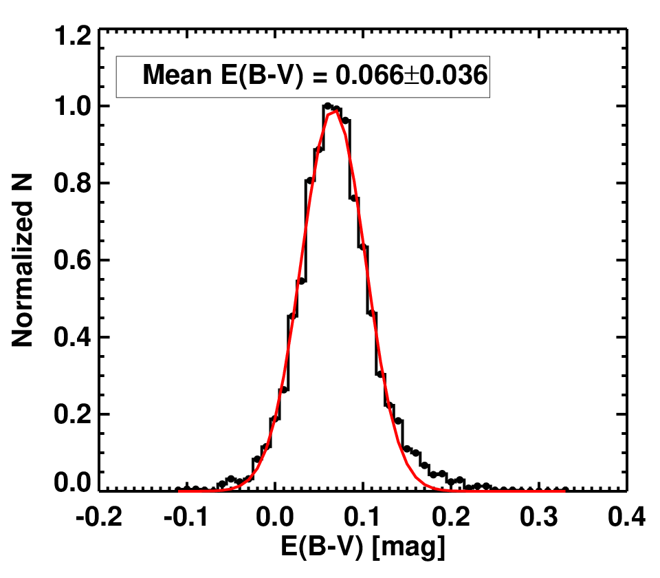
The distance and reddening distributions for the selected sample of RRab stars are shown in Fig. 5. The distribution functions approximate nearly to those of Gaussian profiles. We have fitted a three-parameter Gaussian function to the distance and reddening distribution of these RRab stars. The following values are obtained kpc and mag. Here the uncertainties represent the spread in the population rather than the standard deviation of the mean. On the other hand, weighted averages of the distance and reddening of each of the RRab stars yield the mean distance and reddening as kpc and mag, respectively, where the uncertainties represent the standard errors of the mean values. From reddening distribution plot, it can be seen that for some of the stars, we get unphysical negative reddening values. The number of stars with are found to be which is a very small number () as compared to the total number of stars in the present study. The mean value of reddening of these stars is found to be mag which is statistically not significant and is consistent with zero within the uncertainties. If the stars with negative are set to zero, we get the mean vaues the distance and reddening of the SMC as kpc and mag, respectively. One of the causes of getting the negative reddening values for these stars may be due to the unreliable estimates of their -band mean magnitudes which are underestimated due to the noisy and poorly sampled data points of their light curves or may be due to the propagated uncertainties in their calculated values. These are the two specific cases in which the reddening estimations using equation (6) are likely to yield negative values. Stars with negative values have the values of in the range dex. Mean values of the periods and metallicities of these stars are found to and . The values of the mean period and metallicity of the stars with negative reddening values are respectively higher and lower, as compared to the overall mean values of the total sample and . We have also studied whether there is a trend of these negative reddening values as a function of their periods as well as metallicities but we do not find any clear trend or correlation. In the analysis, we do not ignore those stars with negative reddening values keeping in view of their uncertainties else otherwise this will skew the distribution towards positive reddening values and may lead to biases (Muraveva et al., 2017).
From Fig. 6, it should be noted that the distance and reddening values obtained for the final sample of RRab stars are anticorrelated. The expected behaviour is totally in contrast to what is observed: stars located at larger distances should have higher values of reddening (Nikolaev et al., 2004). This reflects an independent and unbiased determination of these two quantities using the methodologies described in Section 3. Fig. 7 depicts the two-dimensional colour bar plots of the distribution of the reddening values , true distance modulus and true distances for each of the RRab stars. Reddening distribution of the SMC RRab stars is shown in Fig 8. values are binned on a coordinate grid. The average values and their associated errors are given in each bin. The reddening map of the SMC derived from the SMC RRab stars is shown in Fig. 9. The map is produced by computing the average reddening on a grid in coordinates.

Four prominent zones of high internal reddening can be located from the map: one to the south-western part, another one to the north and two others to the south-eastern parts with respect to the centre of the SMC. From the reddening map, one can see that the regions located to the south-eastern part of the centre of the SMC have the highest average values of reddening as compared to the other parts. It can also be seen from the map that the southern part of the SMC has relatively high internal reddening zones as compared to its northern part. One of the highest internal reddening zones is seen to be located near to south-western edge of the SMC.
In a study done using the red clump (RC) stars from the OGLE-II database, Subramanian & Subramaniam (2009) found that the western side of the SMC has high internal reddening. On the other hand using the RC stars and RRab stars of the SMC from OGLE-III database, Haschke et al. (2011) also found that the south-western part of the SMC has higher reddening values. The reddening maps by Haschke et al. (2011); Subramanian & Subramaniam (2012) and the recently obtained reddening map by Muraveva et al. (2017) are in good agreement with our findings. The mean reddening of the SMC mag determined using the present sample of OGLE-IV SMC RRab stars is found to be in good agreement with the values of mag, mag and mag, respectively obtained from the Zaritsky et al. (2002) reddening map using the OGLE-III SMC RRab stars by Deb et al. (2015), from the analysis of Cepheids by Caldwell & Coulson (1986) and from the analysis OGLE-III SMC RRab stars by Haschke et al. (2011). The conversion relation between and is given by . On the other hand, the mean distance to the SMC kpc obtained in the present study is quite consistent with the recent estimates of distance determination to the SMC: kpc by Graczyk et al. (2014), by Inno et al. (2013) using the fundamental mode Cepheids (FU) in the largest NIR band datasets. Furthermore using the NIR datasets for the first overtone Cepheids (FO), Inno et al. (2013) found a true distance modulus of the SMC to be mag. This corresponds to a true distance to the SMC of kpc which is an overestimation of the distance to the SMC when compared with the other values in the literature. Inno et al. (2013) cited this overestimation of the SMC distance due to the lack of precise trigonometric parallax determinations of the Galactic FO Cepheids for distance calibration. Although we have compared the SMC mean distance and reddening value obtained from the Gaussian fit with their respective values available in the literature, these values have been refined to get their intrinsic mean and intrinsic spread using a robust maximum likelihood estimation method as discussed in the next section.

|

|

|
|---|
7 Error Estimation
Each of the parameters and obtained from the light curve analysis of RRab stars using the Fourier decomposition technique will contain standard errors. This will result into the errors in the determination of other parameters dependent on them according to the propagation of error formula (Bevington & Robinson, 2003). Apart from that, each of the observed parameters determined using the empirical and theoretical calibrations will contain systematic errors. Using the propagation of errors formula when the number of observations are large, one can approximately find that the error in the measurement of is , is , is , is , is , is , is . The total uncertainty in values are the errors obtained from the Monte Carlo simulations as well as the quoted systematic uncertainty of as mentioned in equation (13). These uncertainties are added quadratically resulting into a total mean uncertainty of . In order to find a better estimate of the mean and intrinsic spread in the metallicity distribution we use the maximum likelihood estimation method. One of the advantages of maximum likelihood method is that it treats each of the observations independently thus allowing the parameter estimations free from any cumulative systematic errors. The observed metallicity distribution function (MDF) approximates that of the nearly Gaussian profile. The resulting MDF can be thought of as the convolution of an intrinsic Gaussian distribution and a Gaussian error distribution due to heteroscedastic errors for each of the metallicity measurements. The likelihood for obtaining the metallicity values , is given by (Haschke et al., 2012a; Ivezic et al., 2014)
The log likelihood is given by
The maximization of the log likelihood yields the values of the mean metallicity dex and an intrinsic width of the distribution dex for the underlying MDF. Therefore we find the final mean metallicity value to be dex. This value of the mean metallicity of the SMC is in excellent agreement with the value of as found by Skowron et al. (2016). The normalized MDF of RRab stars is shown in Fig. 10. The red colour solid line shows the fitted MDF with the individual metallicity values convolved with the individual Gaussian uncertainties while the blue solid line depicts the intrinsic Gaussian distribution of the MDF. Applying the above procedure of maximum likelihood estimation in the case of mean magnitude and reddening we find the following mean values for the SMC: mag which corresponds to a distance of kpc and mag. Here the uncertainties represent the intrinsic spread rather than the standard deviation of the mean. The values of the distance to the SMC, kpc and kpc, recently obtained by Jacyszyn-Dobrzeniecka et al. (2017) and Muraveva et al. (2017), respectively, are in good agreement with the present study although the values in these two studies are based on entirely different empirical/theoretical relations and calibrations.


8 Period-Color Relation for SMC RRab Stars
Statistically significant large number of SMC RRab stars with their reddening values determined in the present study provides a unique opportunity to explore the various possible relationships between the intrinsic colour and other available light curve parameters of these stars. We try to find out the empirical relationships between and various other parameters involving , and . The various relationships of the following forms are tried:
In order to carry a regressional analysis using the above models, we use function in R11 1 http://www.r-project.org/ statistical package. R is an open source programming language and a software environment for statistical computing and graphics. The results of the regressional analysis are shown in Table 2.
| Relation | -value | |||||||
|---|---|---|---|---|---|---|---|---|
The results thus obtained can be utilised to study the significance of addition of each of the predictor variables on the response variable. The larger value of in all the regressional analysis result indicates that given response variable can be approximated with any of these four relations.But the simplest relationship involving lesser complexity parameters is
| (23) |
where represents the residual standard error per degrees of freedom. Fig. 11 show the vs. plot of the SMC RRab stars. The red solid line denotes the linear fit of the data points obtained from the regressional analysis.
We now test this derived colour relation to find out the mean reddening to the Large Magellanic Cloud (LMC) using the RRab stars taken from the OGLE-IV database. For this, we download the suitable RRab file containing the information about the period (), mean magnitudes in the -band from the LMC OGLE-IV RRab database. We found RRab stars which have mean magnitudes in both the two bands. The observed colour is then calculated from the given mean magnitude information. Then using the period () information taken from the OGLE-IV database, the intrinsic colour for each of the RRab stars were obtained using equation (23). Making use of these information, the reddening value for each of the LMC RRab stars were determined. A three-parameter Gaussian function fitted to the reddening distribution of the yields the mean reddening of the LMC as mag. The mean value of the reddening mag of the LMC found by Haschke et al. (2011) obtained using completely different methods and calibrations is quite consistent with that obtained in this paper. The error in the above reddening estimation represents the actual reddening scatter and the observational error. The mean reddening to the LMC as obtained in this paper using the relation derived with the help of SMC RRab stars is also comparable to mag or as quoted in Caldwell & Laney (1991). Therefore we find that the reddening determination of a galaxy can be made possible from calibrations of the present multicolour photometry of a statistically large number of OGLE RRab stars in the -bands. Nonetheless we caution the reader that this method may not provide the accurate result for an individual star.

9 Three dimensional structure of the SMC
Larger areal coverage and availability of more number of RRab stars in the OGLE-IV phase as compared to the data release of OGLE-III project as well as other earlier OGLE-projects provide a vital means to get an insight into the current understanding of the detailed three dimensional structure of the SMC. This will also facilitate in the refinement of various structure-related parameters of the SMC. Apart from that, the analysis of the distance determination and reddening estimation of each of the SMC RRab stars using their simultaneous light curve data available in -band also provided an unbiased estimate in their determinations. We use the following steps leading to the parameter determinations of the three dimensional structure of the SMC (Deb et al., 2015):
- 1.
The right ascension (), the declination () and the distance () for each of the RRab stars obtained in the present study are converted into the corresponding Cartesian coordinates . The coordinates are obtained using the transformation equations (van der Marel & Cioni, 2001; Weinberg & Nikolaev, 2001; Deb et al., 2015):

Figure 12: Two-dimensional density contours of the SMC RRab stars in the present study. The location of the centre of the SMC is shown as a star symbol. The two-dimensional density contours of the SMC RRab stars in the present study is shown in Fig. 12.
The coordinate system of the SMC disk is the same as the orthogonal system , except that it is rotated around the -axis by the position angle counterclockwise and around the new -axis by the inclination angle clockwise. The coordinate transformations are (van der Marel & Cioni, 2001; Weinberg & Nikolaev, 2001; Deb et al., 2015):
(24) - 2.
The Cartesian coordinate system has the origin in the centre of the SMC at . Here we assume that the axis is pointed towards the observer and -axis lies antiparallel to the -axis. The -axis is taken parallel to the -axis. is the distance between the centre of the SMC and the observer. is the observer-source distance. are the equatorial coordinates of the centre of the SMC. We take the centre of the SMC in the present study as (Subramanian & Subramaniam, 2012; Deb et al., 2015).
- 3.
The errors in each of the Cartesian coordinates () are obtained using the propagation of errors formula (Bevington & Robinson, 2003).
- 4.
The observed distribution of the SMC RRab was modeled by a triaxial ellipsoid. Properties of the ellipsoid are obtained following the principal axes transformation method as described in Deb & Singh (2014).
- 5.
The axes ratios , inclination of the longest axis along the line of sight , position angle of line of nodes along with their associated errors were calculated using the Monte Carlo simulations carried out for steps as discussed in Deb et al. (2015).
- 6.
The normalized distribution functions having iterations of Monte Carlo simulations involving various SMC geometric parameters is obtained after binning with a proper binsize. The normalized distributions of the geometric parameters were found to approximate a Gaussian profile. Three parameter Gaussian profile fitting applied to the each of the distributions yields their mean and values which are taken the as the true values and errors in these parameters.
The normalized distributions of various structural parameters of the SMC obtained following the above steps in the present analysis using RRab stars are shown in Fig. 13. The legend in each of the panels represents the mean and standard deviations of the distributions of the parameters obtained from thre three-parameter Gaussian fits which we quote as the geometrical values of the parameters of the SMC.The following values of the parameters are obtained for the SMC with axes ratios and viewing angle parameters such as and . It should be noted that the position angle defined in equation (24) is measured counterclockwise from the positive x-axis, i.e., from the west direction. The values of the position angles quoted as in this paper are given according to this direction. However, in astronomical convention, position angles are always measured from the north () towards east (). Therefore if measured from north, the position angle of line of nodes will be given by . Also since the position angle is a line, its value can differ by an angle of .
From the results obtained using the principal axis transformation method along with the Monte Carlo method for error estimation we find the lengths of the semi-major, semi-minor and intermediate axes as: kpc, kpc and kpc, where (Deb & Singh, 2014). Following the above results we find that the longest axis viz. the -axis is inclined by from the line of sight, i.e. the line of sight is almost along the -axis of the SMC.

|

|

|
|---|---|---|

|

|
We also applied the simple plane-fitting procedure on the observed three dimensional distribution of the RRab star in Cartesian coordinates . The viewing angle parameters such as inclination () and position angle of line of nodes () are obtained from a plane-fitting procedure of the form (Nikolaev et al., 2004; Deb et al., 2015)
| (25) |
where denotes the number of data points. The inclination angle () can be obtained from the modeled parameters as
Let us now define . Then position angle, can be obtained using Deb et al. (2015)
We now apply a weighted plane-fitting procedure using the mpfitfunc in IDL in order to fit the three dimensional plane of the SMC (Markwardt, 2009; Markwardt, 2012). The fitting procedure yields the following values of the parameters: . This gives the value of and . As measured from the north, the value of will be . In order to validate the results obtained using the IDL routine mpfitfunc, we further develop a Bayesian parameter estimation method in IDL to fit the three dimensional plane of the SMC. The parameter estimation in this case consists of three parts: a plane fitting model, a likelihood function of the data and a prior distribution over the parameters. We have chosen uniform priors for the initial set of parameters. The posterior distribution of the sampling of the model parameters are obtained using the Markov Chain Monte Carlo (MCMC) called the Metropolis-Hasting algorithm (Metropolis et al., 1953; Gregory, 2005). The mean and standard deviations of the posterior distribution of the model parameters are treated as the best fit model parameters and their associated uncertainties. The MCMC iteration was run for steps and the posterior distribution of the sampling of model parameters are noted for each step. The mean and standard deviation of PDF of the posterior probabilities of these model parameters are obtained as: . These parameters yield the values of the viewing angle parameters as: and . If the value of is measured from the north, then its value will be . The fitted plane with the parameters obtained using the Bayesian MCMC analysis is overplotted in Fig. 14. However, the values of the parameters obtained from the three dimensional plane fitting should be taken with caution as the -distribution for the SMC RRab stars has a larger spread and does not actually resemble a plane-like structure. Furthermore using this kind of simple three dimensional plane fitting algorithm we cannot determine the other structural parameters such as the axes ratios of the galaxy.

10 Comparison of SMC parameters obtained using SMOLEC’S (2005) Metallicity Relation and with other studies
We now determine the mean distance and reddening of the SMC using equations (6) and (12) with the values obtained from relation of (Smolec, 2005) which makes use of the - band RRab data:
| (26) |
The above relation was based on the metallicity scale of JK95 metallicity. This linear relation was derived combining the light curve parameters of RRab stars with their complementary spectroscopic metallcities in the range (Smolec, 2005). The relation given by equation (26) is transformed into the metallicity scale of ZW84 using the equation (16). There are other studies, cf., Haschke et al. (2012a); Wagner-Kaiser & Sarajedini (2017) which make use of the following relation given by Papadakis et al. (2000) to convert into the ZW84 scale:
But in a very detailed study by Skowron et al. (2016), it was demonstrated that the use of this relation gives the similar results as those of JK95 around dex, but there exist large offsets of dex at dex and dex at dex, respectively between the two scales. Also since there is no any clear derivation of how the Papadakis et al. (2000) relation was obtained (Skowron et al., 2016), the use of Papadakis et al. (2000) relation is left out in the present study.
All the selection criteria of choosing a clean sample of RRab stars as discussed in Section 4 remain the same except the criterion of metallicity which is taken here as dex. This reduces the original number of RRab stars to for their further analysis. When the present stars are matched with stars obtained in Section 2 the number of common stars found in both are . From the analysis of these stars we have found the following mean values of the parameters of the SMC obtained using the Smolec (2005) metallicity relation: dex, mag, kpc, mag. Here the uncertainties represent the spread of the population rather than the standard deviation of the mean. Making use of the Smolec (2005) metallicity relation the following values of the parameters are obtained for the SMC with axes ratios and viewing angle parameters such as: and . The following relation is obtained:
For this relation denotes the residual standard error per degrees of freedom. This relation is almost identical to the relation given by equation (23) obtained using the Nemec et al. (2013) metallicity relation. Histogram plots of offsets for the and values obtained using the Nemec et al. (2013) (N13) and Smolec (2005) (S05) metallicity relations, respectively into the equations (12) and (6) are shown in Fig. 15. Mean systematic differences of dex, mag, kpc, mag are obtained between the four parameters obtained using the Nemec et al. (2013) and Smolec (2005) relations. The origin of these systematic differences are attributed to the systematic uncertainty in the values obtained using the Smolec (2005) relation as pointed out by Skowron et al. (2016).
The comparison between the distance-related parameters and structural parameters of the SMC obtained in the present study with their corresponding values found in the literature is shown in Table 3. Although we find that the values of the SMC parameters obtained using the Smolec (2005) metallicity relation yield comparable values to those obtained using Nemec et al. (2013) metallicity relation, there are subtle systematic biases present in the mean values of some of the parameters determined using the Smolec (2005) metallicity relation. The bias in the reddening value is almost negligible due to the presence of the expression in the reddening estimation, which involves metallicities in each of the terms. Therefore any systematic bias present in metallicity in one of the terms is reduced/cancelled by the corresponding systematic bias in the other term. In fact we have found that the reddening map constructed based on the relation of Smolec (2005) is quite similar to that obtained based on the Nemec et al. (2013) relation. On the other hand systemtaic bias present in the Smolec (2005) metallicity relation does not get reduced/cancelled in the distance modulus calculation while using the second relation of equation (6) and hence becomes significant. Due to the problem of systematic biases present in the Smolec (2005) metallicity relation towards the low and high metallicity ends, the mean value of the metallicity obtained for the SMC and other parameters derived from it are quite unreliable using this relation (Skowron et al., 2016). Although the consequences of these effects are reduced in a statistical analysis of a large population of RRab stars as in the present study they systematically effect the results on distance determinations using relations. Since the calculation of metallicity using the Nemec et al. (2013) metallicity relation is the most accurate, precise and free from any systematic bias we adopt the results obtained in the present study based on this relation as the final results.

| Reference | (mag) | (kpc) | (mag) | ||||
|---|---|---|---|---|---|---|---|
| - | - | - | - | - | - | ||
| - | - | - | - | - | - | ||
| - | - | - | - | - | - | ||
| - | - | - | |||||
| - | - | - | - | - | |||
| - | - | - | - | - | |||
| - | - | - | - | - | |||
| - | - | - | |||||
| - | - | - | - | ||||
| This work (N13) | |||||||
| This work (S05) |
Caldwell & Coulson (1986); Szewczyk et al. (2009); Haschke et al. (2011); Subramanian & Subramaniam (2012); Haschke et al. (2012b); Inno et al. (2013); Graczyk et al. (2014); Deb et al. (2015); Scowcroft et al. (2016); Jacyszyn-Dobrzeniecka et al. (2017). N13 - Using Nemec et al. (2013) metallicity relation; S05 - Using Smolec (2005) metallicity relation; † Converted into using the relation .
11 Summary and Conclusions
In this paper we have simultaneously utilised both the - and -band light curve data of more than OGLE-IV SMC RRab stars in order to independently determine both the mean distance and reddening of the galaxy. We also study the three dimensional structure of the SMC using the distance distribution of each of the individual RRab stars along with their equatorial coordinates . The availability of a statistically large number of RRab light curve data simultaneously available in the multi-photometric - bands with wider areal coverage being generated for this galaxy from the OGLE-IV photometric survey provides a unique opportunity to develop a more refined understanding of its distance, reddening and three dimensional structure. This newly obtained accurate and precise data have thus helped us in updating our recent knowledge about the distance, reddening and morphological structure of the galaxy. Based on the simultaneous analysis of SMC RRab stars observed in two photometric bands the following results are obtained from the present study:
- 1.
The true mean distance modulus and the mean reddening for the SMC obtained from the light curve analysis of RRab stars are mag and mag, respectively. The uncertainties quoted here represent the intrinsic spread in the population rather than the standard deviation of the mean. The mean distance to the SMC is obtained as kpc. We also find that the distance and reddening values obtained using the methodologies developed in this work are anticorrelated and is thus free from any possible systematic bias.
- 2.
One of the important results of our analysis is the reddening map of the SMC. From the reddening distribution of the SMC RRab stars the reddening map is constructed by computing the average reddening on a grid in coordinates. From the reddening map we find that the southern part of the SMC has relatively more reddening zones as compared to its northern part.
- 3.
The reddening values obtained for each of the individual RRab stars along with their periods () taken from the OGLE-IV database have been utilised to derive a period ()-colour () relation for these stars. The intrinsic colours are obtained from . The following PC relation was obtained:
For this relation denotes the residual standard error per degrees of freedom. The above relation was tested on OGLE-IV LMC RRab stars to find the mean reddening to the galaxy as mag which is consistent with the values for the LMC obtained using other tracers and different methodologies. This is a very useful and significant result on the ground that the above relation was obtained making use of various empirical relations available in the literature (Catelan et al., 2004; Smolec, 2005; Catelan & Cortés, 2008; Nemec et al., 2013; Skowron et al., 2016) and this proves the robust validity of these relations in the application to a large database of RR Lyrae stars. The above relation will prove to be very useful in the estimation of mean reddening value of a host galaxy/globular cluster containing RRab stars quite easily.
- 4.
Approximating the three dimensional distribution of the SMC RRab stars as ellipsoid, we have used the principal axes transformation method (Deb & Singh, 2014; Deb et al., 2015) to find the axes ratios of the SMC: with and . These results are quite consistent with the axes ratios of recently obtained by Jacyszyn-Dobrzeniecka et al. (2017) using a triaxial ellipsoid fitting algorithm originally developed by Turner et al. (1999). Their determinations are based on completely different theoretical and empirical relations which are derived from entirely different calibrations. However the results obtained in this paper using the OGLE-IV dataset are somewhat different than those found by Deb et al. (2015) and Subramanian & Subramaniam (2012) using the entire data set of OGLE-III RRab stars. In the case of semi-major axis ratio , the difference is much more significant, the reason being attributed to the low areal coverage of the SMC obtained during the OGLE-III Project. The results obtained using the the principal axis transformation method along with the Monte Carlo method for error estimation the lengths of the semi-major, semi-minor and intermediate axes are found as: kpc, kpc and kpc, where (Deb & Singh, 2014). This is the first of a series devoted to the determination of the distance, reddening and deciphering the three dimensional structure of the SMC using the available simultaneous -band RRab light curves. In the subsequent papers, we plan to study the distance, reddening and three dimensional structure of the SMC using the Type I and Type II classical Cepheids with the techniques and methodologies developed in this paper. The reddening maps produced independently using the classical Cepheids will provide an opportunity to compare and contrast the reddening map of the SMC produced using the RRab stars in the present study.
Acknowledgments
The author thanks the OGLE-IV team for making their wealthy and invaluable variable star data publicly available for the welfare of the astronomical community. Thanks are due to Science and Engineering Research Board (SERB), Department of Science & Technology (DST), Govt. of India for financial support through a research grant D.O No. SB/FTP/PS-029/2013 under the Fast Track Scheme for Young Scientists in Physical Sciences. The author would like to express his sincere gratitude to Prof. Dhruba J. Saikia, Cotton University for reading the first draft of this manuscript and providing many valuable comments and suggestions. The author acknowledges helpful discussions with Abhijit Saha, Chow-Choong Ngeow and Shashi M. Kanbur while preparing the draft of the manuscript. Lastly, the author thanks the anonymous referee for making various helpful comments and useful suggestions which made the paper significantly relevant. The use of arxiv.org/archive/astro-ph and NASA ADS databases is highly acknowledged.
References
- Beaton et al. (2016) Beaton R. L., et al., 2016, ApJ, 832, 210
- Bevington & Robinson (2003) Bevington P., Robinson D., 2003, Data reduction and error analysis for the physical sciences. McGraw-Hill Higher Education, McGraw-Hill
- Bono et al. (2003) Bono G., Caputo F., Castellani V., Marconi M., Storm J., Degl’Innocenti S., 2003, MNRAS, 344, 1097
- Braga et al. (2015) Braga V. F., Dall’Ora M., Bono G., Stetson P. B., Ferraro I., Iannicola G., Marengo M., Neeley J. e. a., 2015, ApJ, 799, 165
- Burstein & Heiles (1982) Burstein D., Heiles C., 1982, AJ, 87, 1165
- Caldwell & Coulson (1986) Caldwell J. A. R., Coulson I. M., 1986, MNRAS, 218, 223
- Caldwell & Laney (1991) Caldwell J. A. R., Laney C. D., 1991, in Haynes R., Milne D., eds, IAU Symposium Vol. 148, The Magellanic Clouds. p. 249
- Cardelli et al. (1989) Cardelli J. A., Clayton G. C., Mathis J. S., 1989, ApJ, 345, 245
- Carretta et al. (2009) Carretta E., Bragaglia A., Gratton R., D’Orazi V., Lucatello S., 2009, A&A, 508, 695
- Carroll & Ostlie (2006) Carroll B. W., Ostlie D. A., 2006, An Introduction to Modern Astrophysics and Cosmology, second (international) edn
- Catelan & Cortés (2008) Catelan M., Cortés C., 2008, ApJL, 676, L135
- Catelan et al. (2004) Catelan M., Pritzl B. J., Smith H. A., 2004, ApJS, 154, 633
- Deb & Singh (2010) Deb S., Singh H. P., 2010, MNRAS, 402, 691
- Deb & Singh (2014) Deb S., Singh H. P., 2014, MNRAS, 438, 2440
- Deb et al. (2015) Deb S., Singh H. P., Kumar S., Kanbur S. M., 2015, MNRAS, 449, 2768
- Del Principe et al. (2005) Del Principe M., Piersimoni A. M., Bono G., Di Paola A., Dolci M., Marconi M., 2005, AJ, 129, 2714
- Di Criscienzo et al. (2004) Di Criscienzo M., Marconi M., Caputo F., 2004, ApJ, 612, 1092
- Freedman et al. (2001) Freedman W. L., et al., 2001, ApJ, 553, 47
- Graczyk et al. (2014) Graczyk D., et al., 2014, ApJ, 780, 59
- Gregory (2005) Gregory P., 2005, Bayesian Logical Data Analysis for the Physical Sciences. Cambridge University Press, New York, NY, USA
- Haschke et al. (2011) Haschke R., Grebel E. K., Duffau S., 2011, AJ, 141, 158
- Haschke et al. (2012a) Haschke R., Grebel E. K., Duffau S., Jin S., 2012a, AJ, 143, 48
- Haschke et al. (2012b) Haschke R., Grebel E. K., Duffau S., 2012b, AJ, 144, 107
- Inno et al. (2013) Inno L., et al., 2013, ApJ, 764, 84
- Inno et al. (2016) Inno L., et al., 2016, ApJ, 832, 176
- Ivezic et al. (2014) Ivezic Z., Connolly A. J., VanderPlas J. T., Gray A., 2014, Statistics, Data Mining, and Machine Learning in Astronomy: A Practical Python Guide for the Analysis of Survey Data. Princeton University Press, Princeton, NJ, USA
- Jacyszyn-Dobrzeniecka et al. (2017) Jacyszyn-Dobrzeniecka A. M., et al., 2017, Acta Astron., 67, 1
- Jeon et al. (2014) Jeon Y.-B., Ngeow C.-C., Nemec J. M., 2014, in Guzik J. A., Chaplin W. J., Handler G., Pigulski A., eds, IAU Symposium Vol. 301, IAU Symposium. pp 427–428, doi:10.1017/S1743921313014889
- Jurcsik (1995) Jurcsik J., 1995, Acta Astronomica, 45, 653 [JK95]
- Jurcsik & Kovacs (1996) Jurcsik J., Kovacs G., 1996, A&A, 312, 111
- Kanbur et al. (2003) Kanbur S. M., Ngeow C., Nikolaev S., Tanvir N. R., Hendry M. A., 2003, A&A, 411, 361
- Kapakos et al. (2011) Kapakos E., Hatzidimitriou D., Soszyński I., 2011, MNRAS, 415, 1366
- Kovács & Walker (2001) Kovács G., Walker A. R., 2001, A&A, 374, 264
- Madore (1982) Madore B. F., 1982, ApJ, 253, 575
- Majaess (2010) Majaess D. J., 2010, Journal of the American Association of Variable Star Observers (JAAVSO), 38, 100
- Majaess et al. (2011) Majaess D. J., Turner D. G., Lane D. J., Henden A. A., Krajci T., 2011, Journal of the American Association of Variable Star Observers (JAAVSO), 39, 122
- Marconi et al. (2015) Marconi M., et al., 2015, ApJ, 808, 50
- Markwardt (2009) Markwardt C. B., 2009, in Bohlender D. A., Durand D., Dowler P., eds, Astronomical Society of the Pacific Conference Series Vol. 411, Astronomical Data Analysis Software and Systems XVIII. p. 251 (arXiv:0902.2850)
- Markwardt (2012) Markwardt C., 2012, MPFIT: Robust non-linear least squares curve fitting (ascl:1208.019)
- Martínez-Vázquez et al. (2015) Martínez-Vázquez C. E., et al., 2015, MNRAS, 454, 1509
- Metropolis et al. (1953) Metropolis N., Rosenbluth A. W., Rosenbluth M. N., Teller A. H., Teller E., 1953, Journal of Chemical Physics, 21, 1087
- Muraveva et al. (2017) Muraveva T., et al., 2017, preprint, (arXiv:1709.09064)
- Nemec et al. (2011) Nemec J. M., et al., 2011, MNRAS, 417, 1022
- Nemec et al. (2013) Nemec J. M., Cohen J. G., Ripepi V., Derekas A., Moskalik P., Sesar B., Chadid M., Bruntt H., 2013, ApJ, 773, 181
- Nikolaev et al. (2004) Nikolaev S., Drake A. J., Keller S. C., Cook K. H., Dalal N., Griest K., Welch D. L., Kanbur S. M., 2004, ApJ, 601, 260
- Papadakis et al. (2000) Papadakis I., Hatzidimitriou D., Croke B. F. W., Papamastorakis I., 2000, AJ, 119, 851
- Pejcha & Stanek (2009) Pejcha O., Stanek K. Z., 2009, ApJ, 704, 1730
- Piersimoni et al. (2002) Piersimoni A. M., Bono G., Ripepi V., 2002, AJ, 124, 1528
- Salaris et al. (1993) Salaris M., Chieffi A., Straniero O., 1993, ApJ, 414, 580
- Schlegel et al. (1998) Schlegel D. J., Finkbeiner D. P., Davis M., 1998, ApJ, 500, 525
- Scowcroft et al. (2016) Scowcroft V., Freedman W. L., Madore B. F., Monson A., Persson S. E., Rich J., Seibert M., Rigby J. R., 2016, ApJ, 816, 49
- Skowron et al. (2016) Skowron D. M., et al., 2016, Acta Astron., 66, 269
- Smolec (2005) Smolec R., 2005, Acta Astron., 55, 59
- Soszyński et al. (2016a) Soszyński I., et al., 2016a, Acta Astron., 66, 131
- Soszyński et al. (2016b) Soszyński I., et al., 2016b, Acta Astron., 66, 405
- Subramanian & Subramaniam (2009) Subramanian S., Subramaniam A., 2009, A&A, 496, 399
- Subramanian & Subramaniam (2012) Subramanian S., Subramaniam A., 2012, ApJ, 744, 128
- Szewczyk et al. (2009) Szewczyk O., Pietrzyński G., Gieren W., Ciechanowska A., Bresolin F., Kudritzki R.-P., 2009, AJ, 138, 1661
- Turner et al. (1999) Turner D. A., Anderson I., Mason J., Cox M. G., 1999, An Algorithm for Fitting an Ellipsoid to Data
- Udalski et al. (2015) Udalski A., Szymański M. K., Szymański G., 2015, Acta Astron., 65, 1
- Vargas et al. (2014) Vargas L. C., Geha M. C., Tollerud E. J., 2014, ApJ, 790, 73
- Wagner-Kaiser & Sarajedini (2017) Wagner-Kaiser R., Sarajedini A., 2017, MNRAS, 466, 4138
- Weinberg & Nikolaev (2001) Weinberg M. D., Nikolaev S., 2001, ApJ, 548, 712
- Zaritsky et al. (2002) Zaritsky D., Harris J., Thompson I. B., Grebel E. K., Massey P., 2002, AJ, 123, 855
- Zinn & West (1984) Zinn R., West M. J., 1984, ApJS, 55, 45 [ZW84]
- van der Marel & Cioni (2001) van der Marel R. P., Cioni M.-R. L., 2001, AJ, 122, 1807