Exploiting Parallelism in Optical Network Systems: A Case Study of Random Linear Network Coding (RLNC) in Ethernet-over-Optical Networks

The 100/400 GE standards in IEEE 802.3 [1, 2] define Multiple Lane Distribution (MLD) systems with parallel interfaces. In these systems, high-speed Ethernet signals are distributed onto multiple lanes in a round robin fashion, with data rate at 40/100 Gbps perfectly compatible with optical channel rates in Optical Transport Networks (OTNs) [3, 4]. It should be noted that MLD in high-speed Ethernet defines cross-layer system requirements different from inverse multiplexing. The latter technique is standardized in IEEE802.3 as the so-called Link Aggregation, supported by the Link Aggregation Control Protocol (LACP). In optical transport networks (OTN) and synchronous optical network (SONET) standards, the inverse multiplexing is also defined, as Virtual Concatenation (VCAT). In fact, MLD does not require inverse multiplexing techniques, albeit their proven ability to implement dynamic skew compensation mechanism as studied in [5] and [6]. Instead, MLD enables parallel lanes to be mapped to parallel interfaces and channels in the optical layer, allowing the implementation and management of cross-layer interactions, similar to what has been shown Layers 3 and above [7]. Past work also used Layer 2 switching concepts, particularly OpenFlow, in conjunction with multipath TCP (MPTCP) [8].

Our approach utilizes concepts known from similar to multipath routing in layer 3, but extends the same to the network with multiple end-system interfaces. The number of the multiple network end-points can be dynamically configured, which creates not only new network abstractions, but also new routing optimization problems, since the number of end-points is usually matched to the number of routes in the network. In high-speed Ethernet systems, frames are distributed onto multiple lanes (4, or 10 lanes) in a round robin fashion, with data rates perfectly compatible with the corresponding number of optical channel rates in Optical Transport Networks (OTNs) [3, 4].

In the optical layer, the elastic (cognitive, flexible) optical networks, optical transponders (OTP) have evolved from fixed or mixed-line-rate (MLR) to bandwidth-variable (BV) to sliceable-BV [9, 10] to serve various low-capacity (e.g., 40G) and high capacity (400G) demands. The sliceable bandwidth-variable transponders (SBVTs), also called multiflow optical transponder (MF-OTP), maps traffic flows coming from the upper layers (e.g., Internet flows) to multiple optical flows. Moreover, recent work showed that parameters of multiflow optical transponders can be software programmed [11]. These systems are different from parallel network systems, since the Internet traffic flows cannot be dynamically configured to map the optical routes, for instance with an software defined routers.

It should be noted that prior art proposed optimizations to compute multiple paths. In contrast, in our approach abandons the idea of routing optimizations, for the reasons of complexity and also because current multipath routing algorithms cannot be used in network topologies with multiple links between nodes. The latter requires different approach to path analysis, and in our approach we use a combinatorial path analysis for the same. We also show that parallelism can simplify or eliminate routing when used in combination with random linear network coding, which is a significant result.

Previous work on linear network coding focused in general on improving network throughput and reliability. However, significant body of work in the last decade (e.g., [12, 13, 14, 15, 16]) addressed with network coding the end-to-end delays improvement in delay-constrained networks in broadcast and unicast scenarios. In [12], for instance, the delay performance of network coding was studied and compared it to scheduling methods. Lucani et. al, in [13] tailored coding and feedback to reduce the expected delay. Paper [14] studied the problem of minimizing the mean completion delay for instantly decodable network coding. In [15, 16] authors showed that network coding can outperform optimal routing in single unicast setting. More recent works, like [17], presented a streaming code that uses forward error correction to reduce in-order delivery delay over multiple parallel wireless networks. However, none of these works address delay in parallel network systems.

Network-coded multipath routing has been applied for erasure correction [18], where the combined information from multiple paths is transferred on a few additional (parallel) paths. The additional information was used to recover the missing information during decoding.

In optical networks, our previous work [19] proposed for the first time a network coded parallel transmission scheme for high-speed Ethernet using multipath routing. Paper [20] focused on enabling parallel transmission by linear network coding without consideration of data link layer technology. In [21] we presented a preliminary theoretical model to achieve fault tolerance by using 2-parallel transmission and RLNC to achieve better spectral efficiency in the optical layer. Finally, in [22], we showed that utilizing of RLNC significantly improve reliability and security in parallel optical transmission systems.

Our cross-layer approach can be generally based on any symbol based MDS-Codes (Maximum Distance Separable Code), while we decided to use random LNC as a tool owing to the fact that it allows decoupling between code selection and transmission architecture. RLNC encoding and decoding can be perform in a parallel fashion [23], whereas strucutured MDS codes are generally difficult to code or decode in a multithreaded fashion. The distributed nature of the RLNC code construction removes the need for cross-layer coordination when combined with parallelization. Different parallel channels may construct their own codes, and further parallelization takes place with the use of a single coding approach, without the need for state awareness across parallel paths. Our choice of RLNC moreover was motivated by potential use of its recoding capability and design of unified code for a network system in a cross-layer fashion. The composability feature underlies the ability to have cross-layer operation without the need to exchange state or other code-related information across layers. Each layer may, or not, introduce its own coding, composing upon the coding of other layers. Even after repeated coding (recoding), the effect upon the data is of a single linear transformation, requiring no decoding in the network, but a single linear inversion. This makes the combination of RLNC and parallelism especially promising. Note also that RLNC may lend itself to a hybrid use where some of the data may be transmitted uncoded. We do not present that scenario explicitly.

This paper builds on our preliminary works [19, 20]. In extension of the preliminary work, this paper provides

• •

  Derivation of the expected value of the differential delay in arbitrary networks, and between any pair of arbitrary nodes connected with multiple parallel links, enabling routingless (or, random routed) network operation, in cases 1) without coding, 2) with RLNC and 3) with coding redundancy.

• •

  Derivation of occurrence probability of maximum possible differential delay, including cases where network contains multiple links and paths with maximal or/and minimal possible delay, which is a case study of practical relevance;

• •

  A new theoretical framework to queue analysis in end-systems including the derivation of a closed form of expected buffer size at receiver, with and without RLNC, and for an arbitrary distribution of path delays;

• •

  Analysis of the impact of coding redundancy and the level of parallelism on the network performance, and buffer sizing at receiver;

Fig. 1 illustrates a parallel network system architecture envisioned. At the sender, a serial flow of high-speed data units is split into up to $k$ parallel flows (sub-flows, or lanes), whereby each parallel flow is then independently routed over $n$ separate optical channels. Depending on the application, the number of electronic lanes can be perfectly matched to the number of optical channels ($k=n$), whereby the aggregated capacity in the optical layer is always greater or equal to those in the electronic layer. Fig. 1 also illustrates how special functions can be added to each parallel channel, such as adaptive coding features. The input data units (e.g., packets, frames) are encoded using an RLNC encoder. The number of parallel lanes, $k$, and RLNC are related as follows: data units from $k$ parallel flows encoded with the same set of coding coefficients are called a generation, while the number of resulting parallel flows after decoding $n\geq k$ is defined as generation size, here $k=4,n=6$. We refer to the number of resulting parallel lanes, i.e., $n$, as the level of parallelism in end-system ($n=6$). The network topology is such that every node is connected with other nodes over mulitple parallel links (here: 10 parallel links between any pair of nodes). The number of encoded data units $n=6$ is generally equal to the number of parallel paths and interfaces allocated in the network, whereby in our example the source node uses 6 out of 10 parallel interfaces to setup 6 parallel paths. If $n>k$, as we illustrate here, we refer to $r=n-k$ as redundancy, here $r=2$. The decoder starts the decoding as soon as at least $k$ data units from one generation arrived. We envision that forwarding nodes in the middle of network can perform additional recoding of optical flows to the same destination as shown in Fig. 1 (dashed line). With recoding, it is possible to insert additional redundancy and so increase fault tolerance, without decoding.

Fig. 2 shows a typical multi-lane 40Gb/s Ethernet-over-optical network system[1]. In the transmitter, a high speed stream of serial Ethernet frames is split into data blocks of 64b, encoded with 64b/66b line code in Physical Coding Sublayer (PCS), and distributed over $k=4$ virtual Ethernet lanes. For identification of the lane ordering at the receiver, specific alignment markers are inserted in each lane after $M_{L}=16383$ data blocks. After that, each 10GE Ethernet lane is mapped to four optical data units (ODU), here of type 2. The ODU2e method enables the transparent 10GE mapping using an over-clocking approach, whereas extended Generic Framing Procedure (GFP) principles are applied. The ODU signals are then modulated on four optical carriers and transmitted over four optical channels (Path 1, 2, 3, 4). In general, the number of Ethernet virtual lanes and the allocated optical paths do not need to be equal. However, in our model, the OTN concept is assumed to generally map data streams from Ethernet lanes into $n$ ODU2-$n$v or ODU2e-$n$v containers.

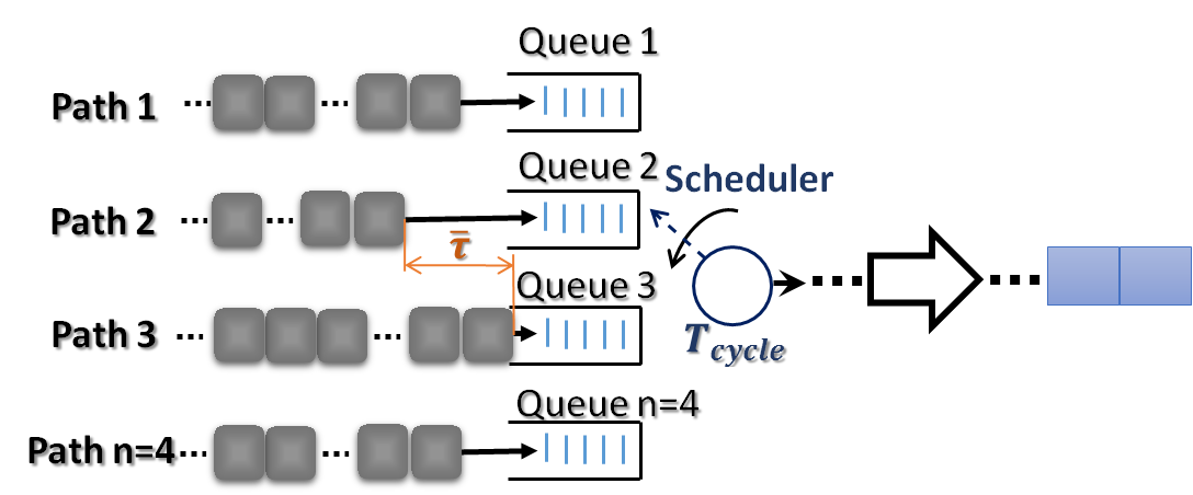
A simplified architecture of the receiver, also according to IEEE802.3ba, is shown in Fig.  2. Here, PCS layer processes the 66b data blocks received to retrieve the original Ethernet frame, which requires multiple processing entities, including lane block synchronization, lane deskew and reorder, alignment removal, etc. (not all shown here). To illustrate this, let us assume that paths $3$ and $4$ are the shortest and the longest path in terms of delay, respectively. For compensation of the resulting inter-lane skew, the data blocks from path $3$ must be buffered in the receiver until data from longer paths arrive, i.e. paths 1, 2, and 4. For compensation, the receiver implements the so-called deskewing and reordering. The deskew function of the PCS is implemented with the input FIFO queues, that store data blocks until the alignment markers of all lanes are received and synchronized. This allows the scheduler to start the lane identification, alignment removal and the reordering to form the original data stream.

Let us now focus on the receiver design with RLNC. A nice feature of RLNC is that it can be implemented without altering the system architecture presented, see dashed box in Fig. 2. The coding process is illustrated in Fig. 3 in more detail. Let us assume an Ethernet frame of $12000$ bits ($1500bytes$) split into $188$ data blocks and then encoded with 64b/66b line code ¹¹ 1 The line code is not to be mistaken for RLNC. The latter is performed over the last 64b after sync header., where we introduce the notation 64b/64b+2b to differentiate between 64 data bits and the 2 bits of the sync header according to [1]. The data blocks are then distributed over $k=4$ virtual PCS lanes so that each sub-flow on defined virtual (parallel) lane contains exactly $47$ data blocks²² 2 In our model of traffic splitting, we assume the bit padding in that case that the data block, or symbol, is incomplete..

Assuming the RLNC coding process is based on symbol size $b=8$ bits, and since blocks contain $64$ data bits excluding the 2 synchronization bits, each coded data block would contain $h=8$ symbols. All $k$ symbols from each parallel lane related to parallel data blocks that are simultaneously encoded with the same set of RLNC coefficients (a generation), while the number of resulting encoded data blocks, i.e., $n$, is defined as generation size. In Fig. 3, each Ethernet frame thus encoded into $47$ generations, while the generation is extended by two redundant blocks resulting in generation size $n=6$. The 2 sync header bits of each data block bypass the RLNC encoder and are added after coding as header in the form 64b/64b+2b+Cb, where C is an additional ID-header.

At the receiver, the reference deskew and reorder model with RLNC is shown in Fig. 4, where transmission is over $n=k=4$ paths similar to traditional Ethernet system (Fig. 2), i.e., without redundancy. Later (Fig. 5), we discuss the system implemented with coding redundancy. The distributed line buffer of the Ethernet system is now organized as a centralized decoding buffer consisting of multiple virtual output queues (VOQ), whereby a new VOQ is created for each generation, each time the first data block of a new generation arrives. The decoder checks the existing VOQ for complete generations, and starts decoding as soon as one generation is complete, whereby all data blocks of a complete generation are decoded in parallel, by running Gaussian elimination. Thus the parallel decoding replaces the line specific deskewing approach of the Ethernet system by taking advantage of the multiplexing gain due to the centralized buffer. After decoding, the data blocks are sent in the correct order, – thus eliminating the need for reordering. That is due to the fact that data blocks are decoded in parallel, while a correct assignment of decoding coefficients to encoded data blocks assures the right order of data blocks. As a result, decoded data blocks are only serialized.

For successful decoding, all data blocks from the same generation $g_{\nu}$ need to be uniquely identified $b_{j_{\nu}},j=1,...,n$. This can be implemented using additional $C=6$ bits in the header to form 72b coded blocks. Each data block of a generation $g_{\nu}$ is identified by the same number $b_{j_{\nu}}=l,j=1,...,n$, whereby we use $L=2^{C}$. At the receiver, the identifier is processed by the scheduler and addresses the correct VOQ $l$. Since ODU2 payload includes 15232 bytes, after $L=64$ sequentially arrived data blocks per lane, the number wrap-round will overwrite the same VOQ with a new generation. This corresponds to the maximium delay difference between lanes to $64tu$, where the time unit (tu) is the transmission time of a data block. For instance, for 10Gbit/s we have $tu=7.2$ns and a maximum delay difference of $446.2$ns, which is far larger than the required $180$ns for Ethernet systems, and thus would be unacceptable. ³³ 3 Note, the 72b=64b/64b+2b+6b block increases the line rate by $12/11$, which requires to develop an efficient GFP method in the OTN layer. A sensible approach to address this is to reuse the Ethernet inherent alignment marker process without adding additional ID-header bits, i.e. $C=0$, also in line with the existing standards. After receiving the first alignment marker, the corresponding lane is marked as reference, the scheduler initialized the VOQ $1$ for the first generation and for each following block of the same line the next VOQ $l$ is generated. In fact this allows to address $M_{L}=16383$ different VOQs, and to compensate delay differences of up to $16383tu$. To limit the buffer space, however, similar to the method with ID-header, we could cyclically overwrite the VOQs after receiving the $L^{th}$ data blocks on the initializing lane, where $L<<M_{L}$. ⁴⁴ 4 The data blocks extracted from an ODU container or its sync header may be erroneous, despite the existence of FEC in the optical layer. In case of a single block errors, the RLNC decoding of one generation will fail. If an alignment marker is erroneous, all data blocks received on the associated lane may be sorted to the wrong VOQ resulting in decoding errors. This error process will be stopped with arrival of the next marker and, thus, re-initialization of VOQs mapping. At the same time, this issue is not different from the erroneous packet handling in the conventional Ethernet system.

The coding coefficients required for encoding and decoding can be selected and distributed by control plane using an out-of-band signaling channel. An in-band signaling method can be used by applying transcoding, as specified in IEEE802.bj. For example with 4 PCS lanes, the 256b/257b transcoding enables us to transmit 35 additional bits after sending 5 blocks of 256b/257b (or after 20 blocks of 64b/66b) per lane (in total, 140 additional bits serially) without increasing the 10GE line rate, which is inline with the Ethernet and OTN standards. Thus, $k=4$ coding vectors each of length 8b can be sent on each lane every 20 64b/66b blocks to the destination, i.e., 20 successive generations are coded with the same coding vector.

In the model that follows, encoding and decoding are applied in the end-systems, i.e., on the Ethernet layer, while optical nodes in the core network simply forward the incoming coded data over reserved outgoing interfaces.

To model the RLNC based end-to-end system, we adopt the network model from [24] representing a network as a directed and acyclic graph $G(V,E)$, where $V$ and $E$ are vertex set and edge set, respectively. The source and destination nodes are denoted as $s\in V$ and $d\in V$, respectively. A distinction is made between incoming and outgoing links of an arbitrary node $v\in V$, which are denoted as a set $\mathcal{E}_{\textrm{in}}(v)$ and $\mathcal{E}_{\textrm{out}}(v)$, respectively. A link $e_{i}$ is an incoming link $e_{i}\in\mathcal{E}_{\textrm{in}}(v)$ of a node $v$, if $head(e_{i})=v$, where $1\leq i\leq|\mathcal{E}_{\textrm{in}}(v)|$, while link $e_{j}$ is an outgoing link $e_{j}\in\mathcal{E}_{\textrm{out}}(v)$ of a node $v$, if $tail(e_{j})=v$, where $1\leq j\leq|\mathcal{E}_{\textrm{out}}(v)|$.

As illustrated in Fig. 3, the traffic sequence, is decomposed into data blocks of the same length, i.e., $h$ symbols each. The linear coding process is performed over a field $F_{2^{b}}$, whereby each symbol has the same length of $b$ bits.

We define time unit (tu) as a discrete time based on the link capacity of the physical link, which can be analyzed as a transmission delay of one data block. Thus, the parallelization, reordering and de-skewing at the end systems can be modeled as a discrete time process. At time $t$, the incoming symbols $\nu$, $\nu=1,2,...,h$, of parallel data blocks $\mathchoice{\vbox{\halign{#\cr\kern-0.7pt\cr$\mkern 2.0mu\displaystyle\mathrel{\mathchoice{{}\hbox{$\displaystyle{\montraitd}$}}{{}\hbox{$\textstyle{\montraitd}$}}{{}\hbox{$\scriptstyle{\montraitd}$}}{{}\hbox{$\scriptscriptstyle{\montraitd}$}}}\mkern-1.5mu\leaders{\hbox{$\displaystyle\mkern 0.0mu\mathrel{\mathchoice{{}\hbox{$\displaystyle{\montraita}$}}{{}\hbox{$\textstyle{\montraita}$}}{{}\hbox{$\scriptstyle{\montraita}$}}{{}\hbox{$\scriptscriptstyle{\montraita}$}}}\mkern 0.0mu$}}{\hfill}\mkern-1.5mu\fldr$\crcr\kern-0.3pt\cr$\hfil\displaystyle x\hfil$\crcr}}}{\vbox{\halign{#\cr\kern-0.7pt\cr$\mkern 2.0mu\textstyle\mathrel{\mathchoice{{}\hbox{$\displaystyle{\montraitd}$}}{{}\hbox{$\textstyle{\montraitd}$}}{{}\hbox{$\scriptstyle{\montraitd}$}}{{}\hbox{$\scriptscriptstyle{\montraitd}$}}}\mkern-1.5mu\leaders{\hbox{$\textstyle\mkern 0.0mu\mathrel{\mathchoice{{}\hbox{$\displaystyle{\montraita}$}}{{}\hbox{$\textstyle{\montraita}$}}{{}\hbox{$\scriptstyle{\montraita}$}}{{}\hbox{$\scriptscriptstyle{\montraita}$}}}\mkern 0.0mu$}}{\hfill}\mkern-1.5mu\fldr$\crcr\kern-0.3pt\cr$\hfil\textstyle x\hfil$\crcr}}}{\vbox{\halign{#\cr\kern-0.7pt\cr$\mkern 2.0mu\scriptstyle\mathrel{\mathchoice{{}\hbox{$\displaystyle{\montraitd}$}}{{}\hbox{$\textstyle{\montraitd}$}}{{}\hbox{$\scriptstyle{\montraitd}$}}{{}\hbox{$\scriptscriptstyle{\montraitd}$}}}\mkern-1.5mu\leaders{\hbox{$\scriptstyle\mkern 0.0mu\mathrel{\mathchoice{{}\hbox{$\displaystyle{\montraita}$}}{{}\hbox{$\textstyle{\montraita}$}}{{}\hbox{$\scriptstyle{\montraita}$}}{{}\hbox{$\scriptscriptstyle{\montraita}$}}}\mkern 0.0mu$}}{\hfill}\mkern-1.5mu\fldr$\crcr\kern-0.3pt\cr$\hfil\scriptstyle x\hfil$\crcr}}}{\vbox{\halign{#\cr\kern-0.7pt\cr$\mkern 2.0mu\scriptscriptstyle\mathrel{\mathchoice{{}\hbox{$\displaystyle{\montraitd}$}}{{}\hbox{$\textstyle{\montraitd}$}}{{}\hbox{$\scriptstyle{\montraitd}$}}{{}\hbox{$\scriptscriptstyle{\montraitd}$}}}\mkern-1.5mu\leaders{\hbox{$\scriptscriptstyle\mkern 0.0mu\mathrel{\mathchoice{{}\hbox{$\displaystyle{\montraita}$}}{{}\hbox{$\textstyle{\montraita}$}}{{}\hbox{$\scriptstyle{\montraita}$}}{{}\hbox{$\scriptscriptstyle{\montraita}$}}}\mkern 0.0mu$}}{\hfill}\mkern-1.5mu\fldr$\crcr\kern-0.3pt\cr$\hfil\scriptscriptstyle x\hfil$\crcr}}}_{i}$ at source node $s\in V$ are generated by the processes $X^{t}(s,i)=x_{i\nu}$, on every virtual lane $i$, denoted as $e_{i}$, $1\leq i\leq k$, $head(e_{i})=s$. The incoming symbols $x_{i\nu}$ are encoded into symbols $y_{j\nu}$, $1\leq j\leq n$, and sent out on each outgoing lane $e_{j}\in E$, $tail(e_{j})=s$. In this model, the RLNC encoder buffers incoming symbols from all $k$ lanes in parallel, and encodes the same with simple linear coding. Thus, the signal carried on an outgoing link $e_{j}$ of source $s$ at time $t+t_{\delta}^{\prime}$ is:

where $t_{\delta}^{\prime}$ is an encoding interval and $a_{ij}$ collected in the matrix $\boldsymbol{A}$ are encoding coefficients from the finite field $F_{2^{b}}$.

At the receiver, the decoded information at time $t+t_{\delta}$ on parallel lane $i$ is modeled as:

where $t_{\delta}$ is decoding interval, $b_{i,j}$ are coding coefficients from the finite field $F_{2^{b}}$ collected in the matrix $\boldsymbol{B}$ [24]. Generally, RLNC can result in linearly dependent combinations, whereby the probability for that combinations is related to the finite field size. The probability of selecting coefficients that do not correspond to a decodable code instance is of the order of $2^{-8}$ [25, 26, 27, 28, 29, 30]. Thus, with high probability, regardless of the number of paths selected, RLNC will lead to a satisfied LNC. The decobability can be verified at the transmitter or receiver. In case an instance of coding coefficent is not decodable, the encoder can readily select another instance, with coefficients selected uniformly at random from the field in which we operate.

The network $G(V,E)$ is modeled as a directed graph with a set of $V$ nodes and $E$ links, whereby each pair of nodes is connected with multiple parallel links. In this topology, it is expected that at least $N\geq n\geq k$ out of $F$ existing parallel links and paths are available between source $s$ and destination $d$, whereby only $n\geq k$ paths are selected for parallel transmission. To derive the likelihood that network can provide $N\geq n$ paths, we use the following model applicable to connection-oriented networks. A network $G(V,E)$ can provide at most $N\leq min\{|\mathcal{E}_{\textrm{out}}(s)|,|\mathcal{E}_{\textrm{in}}(d)|\}$ available parallel paths between nodes $s$ and $d$, while the setup probability of an arbitrary path $\mathcal{P}(s,d)$ over a defined link denoted as $P_{\textrm{setup}}$⁵⁵ 5 Since our motivation is to analyze the differential delay in the network, and the resulting buffer size at the receiver, we do not consider in this paper how various traffic load pattern impact the path setup probability $P_{\textrm{setup}}$.. We approximate the model for blocking probability of the connection request $B(n)$ by assuming that the network load is distributed so that each out of $F$ possible paths can be setup with an equal probability, $P_{\textrm{setup}}$. As a result, the probability, that a path $\mathcal{P}(s,d)$ between $s$ and $d$ cannot be setup, and is blocked, is defined as

Thus, the probability for $N$ available parallel paths out of $F$ existing paths would follow the Binomial distribution, i.e.,

Finally, the transmission request is blocked with probability $B(n)$, when the number of available paths $N$ is lower than the number of outgoing interfaces $n$, i.e., $N<n$.

The mean number of available paths is determined as

On the other hand, the mean number of available for optimization or random selection paths $E\{N|N\geq n\}$, which ensures the successful parallel transmission and is relevant for the buffer analysis in the next Section, can be derived as

As previously mentioned, RLNC can extend the generation size by including $r$ redundant data blocks resulting in $r$ redundant data flows from source. The redundant, i.e., $r$, data blocks are transmitted in parallel with other $k$ data blocks from the same generation. In case of data block loss or network failures, a data block coming from redundant parallel paths can replace any data block from the same generation. We show that this feature is useful not only for fault tolerance but also for reducing the expected value of the differential delay, and thus the buffer size.

The differential delay $\tau$ is typically defined as difference in delays between the longest and the shortest paths $d_{\textrm{max}}$ and $d_{\textrm{min}}$, respectively. We next derive the expected value of differential delay given a number of available paths $N\leq F$ in arbitrary networks, whereby a set of $n$ parallel paths is chosen randomly.

Let’s assume that $n$ parallel paths chosen randomly with the same probability among $N$ available paths form a subset and let’s denote $\mathcal{M}$ as the set of all possible subsets. There are $|\mathcal{M}|=a_{\mathcal{M}}=C_{N,n}$ possible path combinations, where each combination is collected in a subset $\mathcal{M}_{n}(\alpha)\in\mathcal{M}$, $1\leq\alpha\leq a_{\mathcal{M}}$ and appears with same probability $P(\mathcal{M}_{n}(\alpha))=1/a_{\mathcal{M}}$. However, all paths in each subset $\mathcal{M}_{n}(\alpha)$ are sorted so that their corresponding path delays appear in ascended order. This requires to derive an index mapping $l_{m}$, which maps an index $m$, $m=1,2,3,...,n$, used to specify a path $\mathcal{P}_{l_{m}}(\alpha)$ out of the subset $\mathcal{M}_{n}(\alpha)=\{\mathcal{P}_{l_{1}}(\alpha),...,\mathcal{P}_{l_{m}}(\alpha),...,\mathcal{P}_{l_{n}}(\alpha)\}$ to a path $\mathcal{P}_{l}\in G_{\mathcal{P}}$, $l=1,2,...,N$. This also maps the delay $d_{l_{m}}(\alpha)$ of path $\mathcal{P}_{l_{m}}(\alpha)$ to the corresponding component $d_{l}$ of the delay vector $\mkern 2.0mu\textstyle\mathrel{\mathchoice{{}\hbox{$\displaystyle{\montraitd}$}}{{}\hbox{$\textstyle{\montraitd}$}}{{}\hbox{$\scriptstyle{\montraitd}$}}{{}\hbox{$\scriptscriptstyle{\montraitd}$}}}\mkern-1.5mu\leaders{\hbox{$\textstyle\mkern 0.0mu\mathrel{\mathchoice{{}\hbox{$\displaystyle{\montraita}$}}{{}\hbox{$\textstyle{\montraita}$}}{{}\hbox{$\scriptstyle{\montraita}$}}{{}\hbox{$\scriptscriptstyle{\montraita}$}}}\mkern 0.0mu$}}{\hfill}\mkern-1.5mu\fldr$ $\hfil\textstyle d\hfil$ . This ensures, that the increasing index $m$ of each path $\mathcal{P}_{l_{m}}(\alpha)$ corresponds to an increasing path delay $d_{l_{m}}(\alpha)$, $m=1,2,...,n$.

To define such mapping let introduce $\mathcal{N}=\{1,2,...,N\}$ and $\mathcal{N}_{n}=\{\Lambda_{n}\subset\mathcal{N}:|\Lambda_{n}|=n\}$, i.e. the set of all subsets of $\mathcal{N}$ with cardinality $n$. Let us use $\Lambda_{n}(\alpha)$, $\alpha=1,2,...,a_{\mathcal{M}}$, to index each of these subsets. Thus based on paths $P_{l}\in G_{\mathcal{P}}$, the set $\mathcal{M}_{n}(\alpha)$ is given as $\mathcal{M}_{n}(\alpha)=\{\mathcal{P}_{l}:l\in\Lambda_{n}(\alpha)\}$ and the final mapping between path $\mathcal{P}_{l_{m}}(\alpha)\in\mathcal{M}_{n}(\alpha)$ and $\mathcal{P}_{l}\in G_{\mathcal{P}}$ is defined by the index function

where $l\in\mathcal{N}$ and $m=1,2,...,n$. Furthermore, Eq.(8) enables the mapping of paths by the relation $\mathcal{P}_{l_{m}}(\alpha)\equiv\sum_{i}\mathcal{P}_{i}\delta_{\alpha}(i,m)$ and has the property $\sum_{l}\delta_{\alpha}(l,m)=1$. This ensures that each path $\mathcal{P}_{l}\in G_{\mathcal{P}}$ can occur once in the path set $\mathcal{M}_{n}(\alpha)$. For example, assume $n=3$ parallel paths are randomly chosen from the set $G_{\mathcal{P}}$, i.e., $\mathcal{P}_{1},\mathcal{P}_{3}$ and $\mathcal{P}_{4}$. The sorting due to increasing delays defines the mapping to the selected subset shown by the equivalence $\mathcal{M}_{n}(\alpha)=\{\mathcal{P}_{1_{1}}(\alpha),\mathcal{P}_{3_{2}}(\alpha),\mathcal{P}_{4_{3}}(\alpha)\}\equiv\{\mathcal{P}_{1},\mathcal{P}_{3},\mathcal{P}_{4}\}$.

The longest and the shortest paths, $d_{l_{n}}(\alpha)=d_{\textrm{max}}(\alpha)$ and $d_{l_{1}}(\alpha)=d_{\textrm{min}}(\alpha)$, respectively, within chosen set $\mathcal{M}_{n}(\alpha)$ define the differential delay of the path set chosen, i.e.,

As we consider networks with a large number of path sets available, the differential delays depend on the path set chosen, i.e., $\alpha$, $\alpha=1,...,a_{\mathcal{M}}$. The expected value of differential delay $\bar{\tau}=E_{\mathcal{M}}\{\tau(\alpha)\}=E_{\mathcal{M}}\{d_{\textrm{max}}(\alpha)-d_{\textrm{min}}(\alpha)\}$ takes into account all possible paths combinations, as indexed by $\mathcal{M}$, i.e.,

where we use $E_{\mathcal{M}}\{\cdot\}=E\{\cdot\}$ to simplify notation. The expected value $\bar{\tau}$ can be derived knowing the expected delay $E\{d_{m}(\alpha)\}$ of the $m^{th}$ path $\mathcal{P}_{l_{m}}(\alpha)$ over all path sets $\mathcal{M}_{n}(\alpha)$ randomly chosen with probability $P(\mathcal{M}_{n}(\alpha))=1/a_{\mathcal{M}}$. Using the mapping $d_{j_{m}}(\alpha)=\sum_{l}d_{l}\delta_{\alpha}(l,m)$ as specified by Eq. (8), the expected delay of $m^{th}$ path can be derived from

where $p_{l}(m)=1/a_{\mathcal{M}}\sum_{\alpha}\delta_{\alpha}(l,m)$ is the probability, that the $l^{th}$ path $\mathcal{P}_{l}$ with delay $d_{l}$ from $\mkern 2.0mu\textstyle\mathrel{\mathchoice{{}\hbox{$\displaystyle{\montraitd}$}}{{}\hbox{$\textstyle{\montraitd}$}}{{}\hbox{$\scriptstyle{\montraitd}$}}{{}\hbox{$\scriptscriptstyle{\montraitd}$}}}\mkern-1.5mu\leaders{\hbox{$\textstyle\mkern 0.0mu\mathrel{\mathchoice{{}\hbox{$\displaystyle{\montraita}$}}{{}\hbox{$\textstyle{\montraita}$}}{{}\hbox{$\scriptstyle{\montraita}$}}{{}\hbox{$\scriptscriptstyle{\montraita}$}}}\mkern 0.0mu$}}{\hfill}\mkern-1.5mu\fldr$ $\hfil\textstyle d\hfil$ is selected as $m^{th}$ path with delay $d_{l_{m}}(\alpha)$, $m=1,2,...,n$, in a random chosen path set $\mathcal{M}_{n}(\alpha)\in\mathcal{M}$. Using combinatorial theory, in the range $m\leq l\leq N-n+m$ this probability is given by

The detailed derivation of Eq.(12) is in Appendix. Using Eqs. (11)-(12), the expected value of path delay of the $m^{th}$ path of a randomly chosen path set $\mathcal{M}_{n}(\alpha)\in\mathcal{M}$ yields,

where $1\leq m\leq n$. Thus, the expected maximal and minimal path delays over all path combinations are defined as $E\{d_{\textrm{max}}(\alpha)\}=E\{d_{n}(\alpha)\}$ and $E\{d_{\textrm{min}}(\alpha)\}=E\{d_{1}(\alpha)\}$, respectively. Finally, using Eq. (10), the expected value of differential delay can be derived as, i.e.,

To derive further relations, let us define the likelihood that a specific subset $\mathcal{M}_{n}(\alpha)$ is chosen by indicate its dependence on the number $n$ of parallel paths. Since only one out of $a_{\mathcal{M}}$ path combinations is randomly selected for transmission, all path sets and all paths of a set occur with the same probability. Let us denote the probability of an arbitrary paths combination as $P(\mathcal{M}_{n}(\alpha))=\frac{1}{a_{\mathcal{M}}}\equiv P^{\prime}(\alpha,n)$, whereby

where $P_{\mathcal{M}}$ is the probability that an arbitrary path $\mathcal{P}_{l}\in G_{\mathcal{P}}$ is selected for transmission and collected in $\mathcal{M}_{n}(\alpha)$.

Generally, each element $d_{l}$ from $\mkern 2.0mu\textstyle\mathrel{\mathchoice{{}\hbox{$\displaystyle{\montraitd}$}}{{}\hbox{$\textstyle{\montraitd}$}}{{}\hbox{$\scriptstyle{\montraitd}$}}{{}\hbox{$\scriptscriptstyle{\montraitd}$}}}\mkern-1.5mu\leaders{\hbox{$\textstyle\mkern 0.0mu\mathrel{\mathchoice{{}\hbox{$\displaystyle{\montraita}$}}{{}\hbox{$\textstyle{\montraita}$}}{{}\hbox{$\scriptstyle{\montraita}$}}{{}\hbox{$\scriptscriptstyle{\montraita}$}}}\mkern 0.0mu$}}{\hfill}\mkern-1.5mu\fldr$ $\hfil\textstyle d\hfil$ can have value equal to values of their direct neighbors, i.e., $d_{l-1}$ and $d_{l+1}$. Thus, vector $\mkern 2.0mu\textstyle\mathrel{\mathchoice{{}\hbox{$\displaystyle{\montraitd}$}}{{}\hbox{$\textstyle{\montraitd}$}}{{}\hbox{$\scriptstyle{\montraitd}$}}{{}\hbox{$\scriptscriptstyle{\montraitd}$}}}\mkern-1.5mu\leaders{\hbox{$\textstyle\mkern 0.0mu\mathrel{\mathchoice{{}\hbox{$\displaystyle{\montraita}$}}{{}\hbox{$\textstyle{\montraita}$}}{{}\hbox{$\scriptstyle{\montraita}$}}{{}\hbox{$\scriptscriptstyle{\montraita}$}}}\mkern 0.0mu$}}{\hfill}\mkern-1.5mu\fldr$ $\hfil\textstyle d\hfil$ can contain $D_{\textrm{min}}$ and $D_{\textrm{max}}$ elements with minimal and maximal path delays, i.e., $d_{1}=d_{2}=...=d_{D_{\textrm{min}}}$ and $d_{N}=d_{N-1}=...=d_{N-D_{\textrm{max}}+1}$, respectively. Therefore, there maybe many more path combinations $\mathcal{M}_{n}(\alpha)$ yielding a maximal differential delay defined with Eq. (16)

The occurrence probability of $\tau_{\textrm{up}}$ is

where for a path combination $\mathcal{M}_{n}(\alpha)$ we assume, that the $k^{th}$ path $\mathcal{P}_{l_{k}}$ with maximal delay is mapped to one of the $D_{\text{max}}$ paths $\mathcal{P}_{j}\in G_{\mathcal{P}}$, i.e, $d_{l_{k}}(\alpha)=d_{j}$ for $j=N-D_{\text{max}}+1,...,N$. But if $n>N-D_{\text{max}}+1$, the mapping of the path with maximal delay has to be limited to $j\geq max\{n,N-D_{\text{max}}+1\}$. Furthermore, its path with minimal delay, $d_{l_{1}}(\alpha)$, is mapped to one out of $D_{\text{min}}$ paths $\mathcal{P}_{i}\in G_{\mathcal{P}}$ for $i=1,2,...,D_{\text{min}}$. Otherwise for a selected longest path $\mathcal{P}_{j}$, the first path of a set of $n$ path is restricted to paths $\mathcal{P}_{i}\in G_{\mathcal{P}}$ with index $i\leq j-n+1$, thus the mapping of $d_{l_{1}}(\alpha)=d_{i}$ is restricted to the range $i\leq min\{D_{\text{min}},j-n+1\}$. Finally, there are $C_{j-i-1,n-2}$ possible path combinations, whose probability $P^{\prime}(\alpha,n-2)=(P_{\mathcal{M}})^{n-2}$ follows from Eq. (15) and is independent of $\alpha$. Furthermore, the shortest and longest paths in each combination $\mathcal{M}_{n}(\alpha)$, i.e., one or more paths with delays $d_{1}$ and $d_{N}$ from $\mkern 2.0mu\textstyle\mathrel{\mathchoice{{}\hbox{$\displaystyle{\montraitd}$}}{{}\hbox{$\textstyle{\montraitd}$}}{{}\hbox{$\scriptstyle{\montraitd}$}}{{}\hbox{$\scriptscriptstyle{\montraitd}$}}}\mkern-1.5mu\leaders{\hbox{$\textstyle\mkern 0.0mu\mathrel{\mathchoice{{}\hbox{$\displaystyle{\montraita}$}}{{}\hbox{$\textstyle{\montraita}$}}{{}\hbox{$\scriptstyle{\montraita}$}}{{}\hbox{$\scriptscriptstyle{\montraita}$}}}\mkern 0.0mu$}}{\hfill}\mkern-1.5mu\fldr$ $\hfil\textstyle d\hfil$ , respectively, occur with the same probability $P_{i}=P_{j}=P_{\mathcal{M}}$ in all combinations. Thus Eq. (17) can be simplified as follows

When delay vector $\mkern 2.0mu\textstyle\mathrel{\mathchoice{{}\hbox{$\displaystyle{\montraitd}$}}{{}\hbox{$\textstyle{\montraitd}$}}{{}\hbox{$\scriptstyle{\montraitd}$}}{{}\hbox{$\scriptscriptstyle{\montraitd}$}}}\mkern-1.5mu\leaders{\hbox{$\textstyle\mkern 0.0mu\mathrel{\mathchoice{{}\hbox{$\displaystyle{\montraita}$}}{{}\hbox{$\textstyle{\montraita}$}}{{}\hbox{$\scriptstyle{\montraita}$}}{{}\hbox{$\scriptscriptstyle{\montraita}$}}}\mkern 0.0mu$}}{\hfill}\mkern-1.5mu\fldr$ $\hfil\textstyle d\hfil$ contains only two elements with maximal and minimal delay, i.e., $D_{\textrm{min}}=1$ and $D_{\textrm{max}}=1$, the summation is omitted in Eq. (18), which yields

Similar to derivation of Eq. (18), we can additionally derive an occurrence probability of path combinations, where predefined paths $\mathcal{P}_{y}$ and $\mathcal{P}_{x}$ are assumed as longest and shortest paths, respectively, resulting in differential delay $\tau_{x,y}=d_{y}-d_{x}$. That is equivalent to the special case, where $D_{\textrm{min}}$ and $D_{\textrm{max}}$ are irrelevant for probability calculation. Thus, the occurrence probability of the combinations, which contain certain paths $\mathcal{P}_{y}$ and $\mathcal{P}_{x}$ as the longest and the shortest paths, respectively, is

However, when, in a network with $N$ parallel paths, the paths $\mathcal{P}_{y}$ and $\mathcal{P}_{x}$ have delays $d_{y}<d_{N}$ and $d_{x}>d_{1}$, $y<N-D_{\textrm{max}}+1$, $x>D_{\textrm{min}}$, $y-x-1\geq n-2$, the combinations with $\mathcal{P}_{y}$ and $\mathcal{P}_{x}$ as the longest and shortest paths have occurrence probability smaller or equal to the occurrence probability of path combination with maximal differential delay, i.e., $P_{\textrm{up}}\geq P_{{x,y}}$. On the other hand, there can be other path combinations, which do not contain paths $\mathcal{P}_{y}$ and $\mathcal{P}_{x}$ as the longest and shortest paths, but result in the same differential delay value $\tau_{x,y}$. Thus, based on Eq. (18), we can claim that the maximal differential delay $\tau_{\textrm{up}}$ has the larger occurrence probability than any other lower value of differential delay $\tau_{x,y}$ only if $P_{\textrm{up}}>0.5$, which is valid for a large values of $D_{\textrm{min}}$ and $D_{\textrm{max}}$.

As previously mentioned, $k$ parallel lanes can be coded into $n=k+r$ data blocks, and thereafter transmitted over $n$ paths. Thus, network routing redundancy can be directly related to the coding redundancy. Due to the fact, however, that the destination needs to buffer only $k$ out of $n=k+r$ data blocks from the same generation for the decoding start, while any $r$ data blocks arriving later can be ignored, the application of the previous analysis is not straightforward in this case, and needs a few modified expressions of the expected values of the differential delay.

Let us assume that all $n=k+r$ parallel paths are selected randomly with the same probability. For each path set $\mathcal{M}_{n}(\alpha)$ the corresponding delays are sorted as $d_{l_{1}}(\alpha)\leq d_{l_{2}}(\alpha)\leq...\leq d_{l_{k}}(\alpha)\leq d_{l_{k+1}}(\alpha)\leq...\leq d_{l_{m}}(\alpha)\leq...\leq d_{l_{k+r}}(\alpha)$, $d_{l_{m}}(\alpha)=\sum_{i}d_{i}\delta_{\alpha}(i,m)$, $d_{i}$ from $\mkern 2.0mu\textstyle\mathrel{\mathchoice{{}\hbox{$\displaystyle{\montraitd}$}}{{}\hbox{$\textstyle{\montraitd}$}}{{}\hbox{$\scriptstyle{\montraitd}$}}{{}\hbox{$\scriptscriptstyle{\montraitd}$}}}\mkern-1.5mu\leaders{\hbox{$\textstyle\mkern 0.0mu\mathrel{\mathchoice{{}\hbox{$\displaystyle{\montraita}$}}{{}\hbox{$\textstyle{\montraita}$}}{{}\hbox{$\scriptstyle{\montraita}$}}{{}\hbox{$\scriptscriptstyle{\montraita}$}}}\mkern 0.0mu$}}{\hfill}\mkern-1.5mu\fldr$ $\hfil\textstyle d\hfil$ , $1\leq m\leq n$. For successful decoding, the receiver needs to buffer the data blocks arriving from any $k$ paths with least delays, i.e., $d_{l_{m}}(\alpha),m=1,2,...,k$. Thus, in a parallel network system with RLNC, the sender can in fact arbitrarily assign any of the $n$ paths, irrespectively of their related path delays, which eliminates need for routing and complex cross-layer design.

In a parallel network system with linear network coding and $r$ redundant paths, where the path set $\mathcal{M}_{n}(\alpha)$ of $n=k+r$ paths is randomly chosen, a maximal path delay which has to be taken into account at the decoder is bounded as follows

The detailed derivation of Eq. (21) is in Appendix. With Eqs. (21), (12) and (13), an expected maximal path delay follows to be

Similar the expected minimal path delay can be calculated as $E\{d_{\textrm{min}}(\alpha)\}(r)=E\{d_{1}(\alpha)\}$. Finally, with Eq. (22) and using the fact that the number of paths is now given by $n=k+r$ the expected value of differential delay follows to be

where $\bar{\tau}(0)=\bar{\tau}$ simplifies to the result given by Eq. (14).

As a result, the maximal differential delay is

Due to the fact, that the delay vector $\mkern 2.0mu\textstyle\mathrel{\mathchoice{{}\hbox{$\displaystyle{\montraitd}$}}{{}\hbox{$\textstyle{\montraitd}$}}{{}\hbox{$\scriptstyle{\montraitd}$}}{{}\hbox{$\scriptscriptstyle{\montraitd}$}}}\mkern-1.5mu\leaders{\hbox{$\textstyle\mkern 0.0mu\mathrel{\mathchoice{{}\hbox{$\displaystyle{\montraita}$}}{{}\hbox{$\textstyle{\montraita}$}}{{}\hbox{$\scriptstyle{\montraita}$}}{{}\hbox{$\scriptscriptstyle{\montraita}$}}}\mkern 0.0mu$}}{\hfill}\mkern-1.5mu\fldr$ $\hfil\textstyle d\hfil$ can contain $D_{\textrm{max}}$ and $D_{\textrm{min}}$ elements $d_{l}$, which are equal to $d_{N}$ and $d_{1}$, respectively, it is advantageously to consider a special case covered by Eq.(24). If $r<D_{\textrm{max}}$ the maximal relevant delay is given by $d_{N-D_{\textrm{max}}+1}=d_{N-r}=d_{N}$, and $\tau_{\text{up}}(r)=d_{N-D_{\textrm{max}}+1}-d_{1}$ is independent of $r$. Thus, an equivalent form of Eq.(24) is given by $\tau_{\text{up}}(r)=d_{N-max\{r,D_{\textrm{max}}-1\}}-d_{1}$. Using this result and similar to Eq. (17), the occurrence probability of maximal differential delays $\tau_{\textrm{up}}(r)$ is given by Eq. (25).

Due to the $r$ redundant paths, only $k=n-r$ paths are effectively used and the maximal used path delay is determined by $d_{N-max\{r,D_{\textrm{max}}-1\}}$, as discussed above. Thus in contrast to Eq. (17) the $k^{th}$ path $\mathcal{P}_{l_{k}}$ with maximal delay is mapped to one path $\mathcal{P}_{j}\in G_{\mathcal{P}}$ within the range given by $d_{l_{k}}(\alpha)=d_{j}$ for $j=max\{n-r,N-max\{r,D_{\textrm{max}}-1\}\},...,N-r$. Similar, the path with minimal delay, $d_{l_{1}}(\alpha)$, is mapped to one of the paths $\mathcal{P}_{i}\in G_{\mathcal{P}}$ out of the range $i=1,...,min\{D_{\text{min}},j-n+r+1\}$. In accordance with our assumptions, the $r$ redundant paths have a delay larger or equal than the $k^{th}$ path. Now depending on the mapping of the $k^{th}$ path to one path $\mathcal{P}_{j}$, the redundant paths $\mathcal{P}_{l_{k+1}}(\alpha),...,\mathcal{P}_{l_{k+r}}(\alpha)$ will be mapped to paths $\mathcal{P}_{l}\in G_{\mathcal{P}}$ with delays $d_{l}$ out of the range $l=j+1,...,N$. Thus there are $C_{N-j,r}$ path combinations to achieve these mapping, which are combined in subset $\mathcal{M}_{n}(\beta)$. Due to Eq. (15), the probability for the set of $r$ redundant path can be written as $P^{\prime}(\beta,r)=(P_{\mathcal{M}})^{r}$. Similar to Eq. (17), for the remaining $n-r-2$ paths there are $C_{j-i-1,n-r-2}$ combinations whose paths are combined in subset $\mathcal{M}_{n}(\alpha^{\prime})$, where the probability for a set of $n-r-2=k-2$ paths can be written as $P^{\prime}(\alpha^{\prime},n-r-2)=(P_{\mathcal{M}})^{k-2}$. Thus the probability $P_{\textrm{up}}(r)$ simplifies to

For the case, there is only one path with maximal delay, $d_{N-r}$ and only one path with minimal delay, $d_{1}$, i.e $D_{\textrm{max}}=D_{\textrm{min}}=1$, the probability of occurrence of a maximal differential delay can be derived from Eq. (26) as

Compared to the system without redundancy, the receiver experiences a reduction of a maximum differential delay in the network $\boldsymbol{\Delta}^{\text{max}}$, expressed as follows

Additionally, the expected value of differential delay can be reduced by the ratio $\boldsymbol{\Delta}^{\tau}$ determined by Eq. (29).

On the other hand, sending of $r$ redundant data flows over additional $r$ paths presents a capacity and transmission overhead, which we define and later numerically evaluate as

In a parallel network system without RLNC, we refer to the required queue size, as the deskew buffer (Fig. 5). In the system with RLNC, on the other hand, the buffer architecture is based on the virtual output queue (VOQ), referred to as the decoding buffer (Fig. 5). Let us denote the delay difference between the longest and an arbitrary path in a path set $\mathcal{M}_{k}(\alpha)$ as $\tau_{m}(\alpha)\!\!=\!\!d_{l_{k}}(\alpha)-d_{l_{m}}(\alpha)$, $m\!\!=\!\!1,2,...,k$, where $\tau(\alpha)\!\!=\!\!\tau_{1}(\alpha)$ refers to the largest differential delay within the path set and can be determined with Eq. (9).

To analyze the effect of differential delay for $n$ input lanes, in this section we first assume a fixed optimal path pattern $\mathcal{M}_{n}(\alpha_{\textrm{opt}})$ with delays $d_{l_{m}}(\alpha_{\textrm{opt}})$ ordered as $d_{l_{1}}(\alpha_{\textrm{opt}})\leq d_{l_{2}}(\alpha_{\textrm{opt}})\leq...\leq d_{l_{n}}(\alpha_{\textrm{opt}})$. Here, the largest differential delay within the optimal path set is denoted as $\tau(\alpha_{\textrm{opt}})$. Generally, the expected value of the buffer size strongly depends on the paths chosen from vector $\mkern 2.0mu\textstyle\mathrel{\mathchoice{{}\hbox{$\displaystyle{\montraitd}$}}{{}\hbox{$\textstyle{\montraitd}$}}{{}\hbox{$\scriptstyle{\montraitd}$}}{{}\hbox{$\scriptscriptstyle{\montraitd}$}}}\mkern-1.5mu\leaders{\hbox{$\textstyle\mkern 0.0mu\mathrel{\mathchoice{{}\hbox{$\displaystyle{\montraita}$}}{{}\hbox{$\textstyle{\montraita}$}}{{}\hbox{$\scriptstyle{\montraita}$}}{{}\hbox{$\scriptscriptstyle{\montraita}$}}}\mkern 0.0mu$}}{\hfill}\mkern-1.5mu\fldr$ $\hfil\textstyle d\hfil$ .

References

- [1] “Ieee standard for ethernet,” IEEE Std 802.3-2015 (Revision of IEEE Std 802.3-2012), pp. 1–4017, March 2016.
- [2] “IEEE P802.3bs 400 Gb/s Ethernet Task Force,” http://www.ieee802.org/3/bs/index.html.
- [3] “ITU-T Recommendation G.709: Interfaces for the Optical Transport Network (OTN) ,” ITU-T Recommendations.
- [4] “ITU-T Recommendation G.7715/Y.1706 (2002), Architecture and Requirements for Routing in the Automatically Switched Optical Network,” ITU-T Recommendations.
- [5] K. Yang and K. Sivalingam, “Routing in sonet/vcat based optical wdm networks (invited paper),” in BROADNETS, Sept 2009, pp. 1–8.
- [6] Y. Sun, T. Ono, and A. Takada, “Dynamic skew compensation for 40-gb/s/ch multi-wavelength parallel transmission with otn frame,” in OECC/ACOFT, July 2008, pp. 1–2.
- [7] J. Cloud, F. du Pin Calmon, W. Zeng, G. Pau, L. Zeger, and M. Medard, “Multi-path tcp with network coding for mobile devices in heterogeneous networks,” in IEEE VTC, Sept 2013, pp. 1–5.
- [8] R. van der Pol, S. Boele, F. Dijkstra, A. Barczyk, G. van Malenstein, J. H. Chen, and J. Mambretti, “Multipathing with MPTCP and OpenFlow,” in SCC. IEEE, 2012, pp. 1617–1624.
- [9] M. Jinno, H. Takara, Y. Sone, K. Yonenaga, and A. Hirano, “Multiflow optical transponder for efficient multilayer optical networking,” Communications Magazine, IEEE, vol. 50, no. 5, pp. 56–65, 2012.
- [10] T. Tanaka and M. Jinno, “Recent advances in elastic optical networking,” IEICE Transactions on Communications, vol. 97, no. 7, pp. 1252–1258, 2014.
- [11] N. Sambo, G. Meloni, F. Paolucci, F. Cugini, M. Secondini, F. Fresi, L. Potì, and P. Castoldi, “Programmable transponder, code and differentiated filter configuration in elastic optical networks,” Journal of Lightwave Technology, vol. 32, no. 11, pp. 2079–2086, 2014.
- [12] A. Eryilmaz, A. Ozdaglar, and M. Medard, “On delay performance gains from network coding,” in 2006 40th Annual Conference on Information Sciences and Systems, March 2006, pp. 864–870.
- [13] D. E. Lucani, M. Medard, and M. Stojanovic, “On coding for delay - network coding for time-division duplexing,” IEEE Transactions on Information Theory, vol. 58, no. 4, pp. 2330–2348, April 2012.
- [14] S. Sorour and S. Valaee, “On minimizing broadcast completion delay for instantly decodable network coding,” in 2010 IEEE International Conference on Communications, May 2010, pp. 1–5.
- [15] C. C. Wang and M. Chen, “Sending perishable information: Coding improves delay-constrained throughput even for single unicast,” IEEE Transactions on Information Theory, vol. 63, no. 1, pp. 252–279, Jan 2017.
- [16] M. Chen, Y. Tian, and C. C. Wang, “On coding capacity of delay-constrained network information flow: An algebraic approach,” in 2016 IEEE International Symposium on Information Theory (ISIT), July 2016, pp. 2908–2912.
- [17] J. Cloud and M. Medard, “Multi-path low delay network codes,” in 2016 IEEE Global Communications Conference (GLOBECOM), Dec 2016, pp. 1–7.
- [18] N. Maxemchuk, “Dispersity routing: Past and present,” in IEEE Military Communications Conference. IEEE, 2007, pp. 1–7.
- [19] X. Chen, A. Jukan, and M. Medard, “A novel network coded parallel transmission framework for high-speed ethernet,” in Global Communications Conference (GLOBECOM), 2013 IEEE, Dec 2013, pp. 2382–2387.
- [20] X. Chen, A. Engelmann, A. Jukan, and M. Medard, “Linear network coding reduces buffering in high-speed ethernet parallel transmission systems,” IEEE Communications Letters, 2014.
- [21] X. Chen, A. Jukan, and M. Medard, “Linear network coding and parallel transmission increase fault tolerance and optical reach,” in International Conference on Communications, 2015 IEEE, June 2015, pp. 2382–2387.
- [22] A. Engelmann and A. Jukan, “Balancing the demands of reliability and security with linear network coding in optical networks,” in 2016 IEEE International Conference on Communications (ICC), May 2016, pp. 1–7.
- [23] P. Vingelmann and F. H. P. Fitzek, Networks for Grid Applications: Third International ICST Conference, GridNets 2009, Athens, Greece, September 8-9, 2009, Revised Selected Papers. Berlin, Heidelberg: Springer Berlin Heidelberg, 2010, ch. Implementation of Random Linear Network Coding Using NVIDIA’s CUDA Toolkit, pp. 131–138.
- [24] R. Koetter and M. Médard, “An algebraic approach to network coding,” in IEEE/ACM Trans. Networking, vol. 11, 2003, pp. 782–295.
- [25] O. Trullols-Cruces, J. M. Barcelo-Ordinas, and M. Fiore, “Exact decoding probability under random linear network coding,” IEEE Communications Letters, vol. 15, no. 1, pp. 67–69, January 2011.
- [26] T. Ho, M. Médard, R. Koetter, D. Karger, M. Effros, J. Shi, and B. Leong, “A Random Linear Network Coding Approach to Multicast,” IEEE Transactions on Information Theory, vol. 52, no. 10, pp. 4413–4430, October 2006.
- [27] C. F. Chiasserini, E. Viterbo, and C. Casetti, “Decoding probability in random linear network coding with packet losses,” IEEE Communications Letters, vol. 17, no. 11, pp. 1–4, November 2013.
- [28] F. Li, “Exact decoding probability of random linear network coding for combinatorial networks,” Wuhan University Journal of Natural Sciences, vol. 20, no. 5, pp. 391–396, 2015.
- [29] H. Han, D. Peng, and L. Wang, “Iet networks,” Upper bounds for the failure probability of random linear network coding for multicast network, vol. 2, no. 4, pp. 181–187, December 2013.
- [30] K.-H. Lee, J.-H. Kim, and S. Cho, Wireless Algorithms, Systems, and Applications: 9th International Conference, WASA 2014, Harbin, China, June 23-25, 2014. Proceedings. Springer International Publishing, 2014, ch. RLNC in Practical Wireless Networks, pp. 194–204.
VII Appendix
VII-A Derivation of Eq.(12)
The delays of the paths are sorted in the ascending order, i.e., . In the same way, a subset of paths have delay values . Due to this ordering, it is obviously that the delay of the path can only be mapped to delays from in the range . Now let us assume, that the path of an arbitrary subset is mapped to the path with delay . Then there are paths with delays whose delays are smaller or equal to , which can be mapped to a set of paths with delays . Since there are possible combinations for this mapping.
Similarly, there are paths with delays whose delays are larger or equal as , which can be mapped to a set of paths with delays . Since there are possible combinations for this mapping. Overall, we have in total combinations with equal probability, where the path with delay from is selected as path with delay , thus this probability is given by
VII-B Derivation of Eq.(21)
The routing over network is implemented over paths and redundant paths in parallel. Thus, paths from existing paths can be chosen randomly. For decoding to start, the receiver needs only data blocks from any those paths that are shorter than the remaining paths. Since the vector is sorted in ascending order as , a maximal path delay that has an impact on decoding start is , and, thus, the delay from defines a minimal possible value of a maximal path delay. On the other hand, the last delays from vector can be any delay , . Since only paths with delays , , …, provide data blocks relevant for decoding to start, the path delay is a maximum delay, which a receiver experiences.