MUBs and SIC-POVMs of a spin-1 system from the Majorana approach

where $a_{iz}=\vec{z}\cdot\vec{a_{i}}$ $(i=1,2)$. These equations imply that $a_{2z}=-a_{1z}$ and $\vec{a_{1}}\cdot\vec{a_{2}}=-3a_{1z}^{2}$; in other words, they imply that the vectors $\vec{a_{1}}$ and $\vec{a_{2}}$ lie on the upper and lower halves of a double-cone of semi-vertex angle $\theta$ (say) and make an angle of $\cos^{-1}(-3\cos^{2}\theta)$ with each other, where $\cos^{-1}(\frac{1}{\sqrt{3}})\leq\theta\leq\frac{\pi}{2}$ (see Fig.3). We will refer to these states as “double-cone” states. There are actually two different types of double-cone states on any double-cone and they can specified in terms of their angular coordinates as

where $\phi_{\theta}=\cos^{-1}(2\cot^{2}\theta)$ is an acute angle. We will refer to $\phi_{\theta}$ as the “twist angle” because it is the angle by which the lower vector is rotated on its double-cone from its straight line position with the upper vector. This rotation is in the clockwise sense for the state $D^{R}$ and the counter-clockwise sense for $D^{L}$; thus these states have different chiralities, as noted in their superscripts $R$ and $L$. The states $D^{R}(\theta,\phi)$ and the $D^{L}(\theta,\phi)$ both form a continuous family for $0\leq\phi<2\pi$, but no member of one coincides with any member of the other.

The double-cone states are particular examples of D-states, and they are in fact the only types of D-states we ever have to consider in connection with MUBs. The double-cone states have some important properties that we state in the form of a number of propositions:

Proposition 1. Let $\Theta$ be the operation of inverting the M-vectors of a state in the origin⁶⁶ 6 The physical significance of this operation is that it corresponds to time-reversal.. Then $\Theta D^{R}(\theta,\phi)=D^{L}(\theta,\phi-\phi_{\theta})$.

Proof: This is easily seen from (9) on noting that $\theta\rightarrow\pi-\theta$ and $\phi\rightarrow\phi+\pi$ under inversion and that the order of the arguments of a double-cone state is irrelevant.   $\Box$

In words, this relation says that inverting the vectors of $D^{R}(\theta,\phi)$ in the origin produces the same state that would be obtained by rotating the vectors of $D^{L}(\theta,\phi)$ clockwise about the z-axis by the angle $\phi_{\theta}$.

Proposition 2. Double-cone states are chiral for $\cos^{-1}(1/\sqrt{3})<\theta<\pi/2$ but lose their chirality at the two limits of this range.

Proof: The chirality within this range was already pointed out earlier, so we just need to look at the two limits. At the lower limit, $\theta=\cos^{-1}(1/\sqrt{3})=54.74^{\circ}$, the twist angle goes to zero and the state degenerates into an A-state, which is not chiral. And at the upper limit, $\theta=\pi/2$ or $3\pi/2$, and the double-cone flattens out into a plane with the M-vectors becoming orthogonal; the chirality is again lost because the inverse of a state in the origin can be obtained by rotating the vectors of the original state by a half-turn about the z-axis. We will dispense with the superscripts $R$ and $L$ for these two limiting cases of the double-cone states.   $\Box$

Proposition 3. The overlap of the states $D^{R}(\theta,0)$ and $D^{R}(\theta,\phi)$ vanishes only for $\phi=2\pi/3$ or $4\pi/3$. The same is true of the $L$ states.

Proof: On using (5), the orthogonality condition for a pair of $R$ or $L$ states takes the form

from which the result follows immediately.  $\Box$

Remark. Note that the three states $D^{R}(\theta,0)$, $D^{R}(\theta,2\pi/3)$ and $D^{R}(\theta,4\pi/3)$ form a basis, as do the corresponding $L$ states. The double-cone states at the two boundaries of the range, which are not chiral, also have this property.

Proposition 4. The only values of $\phi$ for which the states $D^{R}(\theta,0)$ and $D^{R}(\theta,\phi)$ become unbiased are $\pm\cos^{-1}(\frac{\sqrt{3}-1}{2})=\pm 68.53^{\circ}$. The same is true of the $L$ states.

Proof: On using (6), the unbiasedness condition for either the $R$ or $L$ states takes the form

from which the result follows immediately.   $\Box$

and the quantities $c_{1},c_{2},d_{1},d_{2},c_{3}$ and $c_{4}$ are defined as

The function $F(\phi)$ can be cast into a simpler form by the variable change $\phi^{\prime}=\phi-\phi_{0}$, with $\phi_{0}$ being a suitable constant. Then it takes the form

If one chooses $\phi_{0}$ so that $c^{\prime}_{1}=c^{\prime}_{2}=0$, then (19) reduces to

However for this to happen both the conditions

must be satisfied. These conditions can be satisfied simultaneously only if $d_{1}(c_{2}d_{1}-c_{1}d_{2})=c_{1}(c_{1}c_{2}+d_{1}d_{2})$, but it is easily verified that this is the case and one then sees, with the aid of (15) and (16), that

With $\phi_{0}$ thus fixed, the coefficients in (23) assume the values

Eqs.(23),(26),(27) and (28) are the form of the function $F$ that we will employ in the subsequent analysis. This form is particularly convenient because it reveals $F$ to be an even function of $\phi^{\prime}$ with two unequal maxima and two equal minima (see Fig.4). The two propositions to be proved now can be appreciated better in the context of this figure.

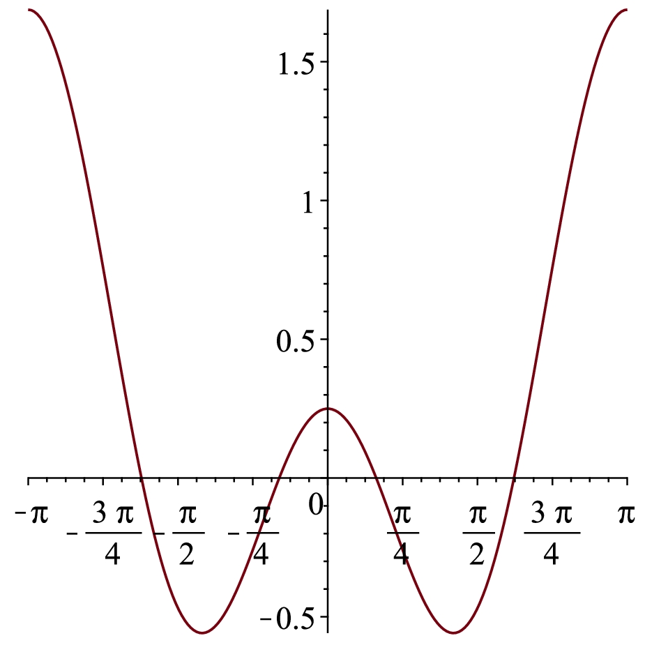
Proposition 5. Two states on different double-cones can never be orthogonal.

Proof: We must show that $F(\phi^{\prime})+c_{3}>0$ for all $\phi^{\prime}$ if $\theta_{1}\neq\theta_{2}$. On putting the derivative of $F$ with respect to $\phi^{\prime}$ equal to zero we find that the maxima of $F$ occur at $\phi^{\prime}=0$ and $\pi$ and the minima at $\phi^{\prime}=\cos^{-1}\Big(-d^{\prime}_{1}/2d^{\prime}_{2}\Big)$. The value of $F(\phi^{\prime})+c_{3}$ at the minimum is $-\frac{{d^{\prime}_{1}}^{2}}{4d^{\prime}_{2}}+c^{\prime}_{3}+c_{3}$, and using (17),(18),(26),(27) and (28) allows the value of the minimum to be written as

We must now show that this expression is positive definite for $\theta_{1}\neq\theta_{2}$. However this follows from the fact that (29) is symmetrical in the parameters of the two states and so achieves its extreme (here minimum) value when $\theta_{1}=\theta_{2}$ and $\phi_{1}=\phi_{2}$; but this minimum value is zero, and so it follows that (29) is positive definite for $\theta_{1}\neq\theta_{2}$, which proves the claim.   $\Box$

Remark 1. The geometrical meaning of this proposition can be understood by looking at Fig.4: essentially, adding the constant $c_{3}$ to the function $F(\phi^{\prime})$ raises it vertically so that both its (equal) minima lie above the $x$-axis.

Remark 2 (a corollary). When $\theta_{1}=\theta_{2}$, the two minima of $F$ just touch the $x$-axis at $\phi^{\prime}=\pm 2\pi/3$ and, in addition, $\phi_{0}=(\phi_{2}-\phi_{1})/2=0$; together these results imply that the states orthogonal to a given state lie on the on the same double-cone as it and are rotated from it by angles of $\pm 2\pi/3$ about the cone axis, which is just the result proved in Proposition 3. However we are now in a position to make the stronger statement that any double-cone state is a member of a unique basis consisting of it and the two other states obtained from it by rotations of $\pm 2\pi/3$ about the cone axis. We will use the notation $\big[D^{R,L}(\theta,\phi)\big]$ for such a basis, identifying it by its first member, with the understanding that the other two members are $D^{R,L}(\theta,\phi+2\pi/3)$ and $D^{R,L}(\theta,\phi+4\pi/3)$.

Remark 3. A much quicker proof of this proposition can be given if we represent the states as rays in Hilbert space. Let $1$ be a state on the double-cone $\theta_{1}$ and $2$ a state on a different double-cone $\theta_{2}$ that is assumed to be orthogonal to 1. We can represent $1$ and $2$ by the rays $(1,0,0)$ and $(0,1,0)$. Now rotate both $1$ and $2$ on their double-cones by the angle $2\pi/3$ so that they go into the states $1^{\prime}$ and $2^{\prime}$. But, from Proposition 3, $1^{\prime}$ is orthogonal to $1$ and $2^{\prime}$ to $2$, so these states can be represented as $1^{\prime}=(0,\alpha_{1},\alpha_{2})$ and $2^{\prime}=(\beta_{1},0,\beta_{2})$. However the M-vectors of $2^{\prime}$ and $1^{\prime}$ bear the same relationship to each other as those of $2$ and $1$, and so $2^{\prime}$ and $1^{\prime}$ must be orthogonal. But the inner product of $1^{\prime}$ and $2^{\prime}$ is ${\beta_{2}}^{*}\alpha_{2}$, which can be zero only if $\alpha_{2}=0$ or $\beta_{2}=0$; however the former choice makes $1^{\prime}=2$ and the latter makes $2^{\prime}=1$, neither of which is permissible, so it follows that $1$ and $2$ cannot be orthogonal, as originally assumed.

Let us pause to take stock of where we are at. We chose the initial basis of the MUB to be a CAC basis and we have now shown, as a corollary of Proposition 5, that all the remaining bases must be double-cone bases of the form $\big[D^{R,L}(\theta,\phi)\big]$. It remains to see how many bases of this kind we can pick that will form a MUB together with the original CAC basis. The answer to this question is given in the next proposition.

Proposition 6. Let $\big[D^{R}(\theta_{1},0)\big]$ be a double-cone basis, for an arbitrary value of $\theta_{1}$. Then it is always possible to find two other bases, lying on the double-cones $\theta_{2}$ and $\theta_{3}$ that, together with $\big[D^{R}(\theta_{1},0)\big]$ and the CAC basis, form a MUB. To fix $\theta_{2}$ and $\theta_{3}$, let $y=\cos^{2}\theta_{1}$ and consider the quartic equation

This equation always has two real roots, $x_{2}=\cos^{2}\theta_{2}$ and $x_{3}=\cos^{2}\theta_{3}$, that fix $\theta_{2}$ and $\theta_{3}$. To determine the bases on these double cones, consider the equation

where $j=2$ or $3$, $\phi_{1},\phi_{2}$ and $\phi_{3}$ are the (acute) twist angles associated with the double-cones $\theta_{1},\theta_{2}$ and $\theta_{3}$ and $\sigma_{1}$ and $\sigma_{2}$ can each take on the values $+1$ and $-1$. For a given $j$, one can use the value of $\theta_{j}$ found from (30) to solve (31) for $\phi_{j}$. However one finds that there is a solution for only one combination of values of $\sigma_{1}$ and $\sigma_{2}$ and that it determines a basis on the double-cone $\theta_{j}$ in the manner indicated in the following table:

The phase offset $\phi_{0}$ in Table 1 is given by (25), which in the present case can be written as $\phi_{0}=\frac{1}{2}\big(\phi_{j}-\phi_{1})$, where $\phi_{j}$ is the twist angle associated with the double-cone $\theta_{j}$.

Admittedly this result is not simple. However it has the virtue of delivering the entire MUB resulting from the choice of an initial double-cone state (on the cone $\theta_{1}$) in a single, easily implemented, package. Deferring the proof of this proposition to Appendix 2, we concentrate here on trying to convey a feeling for it and then unpack some of the special cases contained in it.

The quartic equation (30) that gives rise to the MUB may seem rather complicated at first, but it has an underlying simplicity that allows one to grasp the nature of its solutions. A close inspection shows that it has the form $f(x,y)=0$, where $f(x,y)$ is a symmetrical function of $x$ and $y$. A contour plot of (30) is shown in Fig.5 over the entire region $0\leq x,y\leq\frac{1}{3}$ in which double-cones exist. It is seen to have the shape of a fat boomerang that is symmetrical about the line $y=x$. If we take $y=\cos^{2}\theta_{1}$ and draw a horizontal line corresponding to this value of $y$, it cuts the curve at two points that determine the other two double-cones, $\theta_{2}$ and $\theta_{3}$, of the MUB. However, if $y=0$ or $\frac{1}{3}$, the line is tangent to the curve at a single point that leads to only one additional double-cone.

The MUBs with three double-cones are chiral and have a mix of R and L type bases. Inverting the M-vectors of any such MUB in the origin leads to another MUB of the opposite handedness, and the two together form an enantiomorphic pair. However the special MUBs consisting of just two double-cones are not chiral, as we now demonstrate.

Consider first the MUB defined by the condition $y=1/3$, for which the quartic reduces to

This equation has a pair of double roots, $\frac{2\sqrt{3}}{3}-1$ and $-\frac{2\sqrt{3}}{3}-1$, of which only the former is positive and acceptable. Thus this MUB has two double-cones of angles $\theta_{a}=\cos^{-1}(\sqrt{\frac{2}{\sqrt{3}}-1})$ and $\theta_{b}=\cos^{-1}(1/\sqrt{3})$. We can work out the bases on these double cones from (31) and Table 1, and the results are given in Table 2. We see that the basis on $\theta_{b}$ is its own inverse in the origin (which we already knew from Proposition 2) while the two bases on $\theta_{a}$ are the inverses of each other. Thus the MUB as a whole is inversion symmetric and not chiral. We call this MUB MUB-1 to distinguish it from MUB-2 that we will introduce shortly. In addition to listing the M-vectors of this MUB, we have also listed the corresponding rays in Hilbert space (see Appendix 3 for an explanation of how the rays can be worked out). The last column shows the rays in the simplified form in which they are sometimes quoted; if we denote by $Z$, $X$, $Y=XZ$ and $W=XZ^{2}$ the operators of the qutrit Pauli group, then the bases in the four blocks are the simultaneous eigenstates of the pairs of commuting operators ($Z,Z^{2}$), ($Y,Y^{2}$), ($W,W^{2}$) and ($X,X^{2}$), respectively.

Consider next the MUB defined by $y=0$, for which the quartic reduces to

The solution again consists of a pair of double roots, $2\sqrt{7}-5$ and $-2\sqrt{7}-5$, of which only the former is acceptable and leads to the double-cone $\theta_{d}=\cos^{-1}(\sqrt{2\sqrt{7}-5})$. The other double-cone, corresponding to $y=0$, has angle $\pi/2$ and is actually the x-y plane. We can work out the bases on these double-cones from (31) and Table 1 and the results are given in Table 2. One sees that the double-cone $\theta_{d}$ has two bases that are the reflections of each other in the horizontal plane while the flattened double-cone has a single basis that is its own reflection. Thus the MUB as a whole has reflection symmetry is not chiral. The rays of this MUB are also listed and, again, a simple unitary transformation can be used to turn them into the simple form shown in the last column.

Finally we address an important point. We have shown how to construct an infinite number of MUBs by starting from an arbitrary state on the double-cone $\theta=\cos^{-1}\sqrt{y}$, for any $0\leq y\leq\frac{1}{3}$. One can ask if these MUBs are independent or related to each other. The answer is that they are all unitarily equivalent to each other under a “phasing” transformation that we now describe. Consider the rays of MUB-1, shown in last column of Table 1. Applying the unitary transformation $U=\text{diag}(1,1,e^{i\psi})$ to these rays, with $0\leq\psi<2\pi$, allows us to generate all the MUBs yielded by our construction. For $\psi=0,\frac{2\pi}{3}$ or $\frac{4\pi}{3}$ we get MUB-1, which has inversion symmetry; for $\psi=\pi$ we get MUB-2, which has reflection symmetry; and for all other $\psi$ we get MUBs that are chiral. The MUBs for $\psi=\pi-\psi_{0}$ and $\psi=\pi+\psi_{0}$ are the inverses of each other in the origin (up to a rotation about the z-axis) for all $\psi_{0}$ in the open interval $0<\psi_{0}<\pi$, with the exception of the point $\frac{2\pi}{3}$. In conclusion a spin-1 system has a unique MUB, although it can assume an infinite number of guises when viewed in the Majorana representation.

References

- (1) I.D.Ivanovic: Geometrical description of quantal state determination. Journal of Physics A 14 3241 (1981).
- (2) W.K.Wootters and B.Fields: Optimal state-determination by mutually unbiased measurements. Annals of Physics 191 363 (1989).
- (3) W.K.Wootters: Picturing qubits in phase space. ArXiv: quant-ph/0306135v4 (2003).
- (4) W.K.Wootters: Quantum measurements and finite geometry. ArXiv: quant-ph/0406032v3 (2004).
- (5) K.S.Gibbons,M.J.Hoffman and W.K.Wootters: Discrete phase space based on finite fields. Phys. Rev. A70 062101 (2004).
- (6) S.Bandyopadhyay, P.Boykin, V.Roychowdhury and F.Vatan: A new proof for the existence of mutually unbiased bases. Algorithmica 34 512 (2002).
- (7) J.Lawrence, C.Brukner and A.Zeilinger: Mutually unbiased binary observable sets on N qubits. Phys. Rev. A65 032320 (2002).
- (8) T.Durt, B.G.Englert, I.Bengtsson and K.Zyczkowski: On mutually unbiased bases. International Journal of Quantum Information 12 535 (2010).
- (9) P.Mandayam, S.Bandyopadhyay, M.Grassl and W.K.Wootters: Unextendible mutually unbaised bases from Pauli classes. Quant. Inf. Comput. 14 0823-0844 (2014).
- (10) S.Brierley, S.Weigert and I.Bengtsson: All Mutually Unbiased Bases in Dimensions Two to Five. Quantum Information and Computation 10 0803 (2010).
- (11) M.Weiner: A gap for the maximum number of mutually unbiased bases. Proceedings of the American Mathematical Society 141 1963-1969 (2013).
- (12) G.Zauner: Quantum Designs - Foundations of a Non-commutative Theory of Designs. International Journal of Quantum Information 09 445-507 (2011).
- (13) P. W. H. Lemmens and J. J. Seidel: Equiangular lines, J. Algebra 24, 494 (1973).
- (14) J.M.Renes, A.Blume-Kohout, A.J.Scott and C.M.Caves: Symmetric informationally complete quantum measurements. Journal of Mathematical Physics 45 2171 (2004).
- (15) D.M.Appleby: Symmetric informationally complete-positive operator valued measures and the extended Clifford group. J. Math. Phys. 46 052107 (29pp.) (2005).
- (16) G.N.M.Tabia and D.M.Appleby: Exploring the geometry of qutrit state space using symmetric informationally complete probabilities. Phys. Rev. 88 012131 (2013).
- (17) D.M.Appleby, C.A.Fuchs and H.Zhu: Group theoretic, Lie algebraic and Jordan algebraic formulations of the SIC existence problem. Quantum Information and Computation 15 No.1-2, 61-94 (2015).
- (18) D.M.Appleby, I.Bengtsson, S.Brierley, M.Grassl, D.Gross and J-A.Larsson: The monomial representations of the Clifford group. Quantum Information and Computation 12 No.5-6, 0404-0431 (2012).
- (19) H.Zhu, Y.S.Teo and B-G. Englert: Structure of Two-qubit Symmetric Informationally Complete POVMs. Phys. Rev. A82 042308 (2010).
- (20) H.Zhu: SIC POVMs and Clifford groups in prime dimensions. J. Phys. A: Math. Theor. 43 305305 (2010).
- (21) C.A.Fuchs: Quantum Mechanics as Quantum Information (and only a little more). ArXiv: 0205039v1 (2002).
- (22) L.Hughston and S.Salamon: Surveying points in the complex projective plane. ArXiv: 1410.5862v2[math.DG] (2015).
- (23) S.G.Hoggar: t-Designs in Projective Spaces. Europ. J. Combinatorics 3 233-254 (1982).
- (24) J.Jedwab and A.Wiebe: A simple construction of complex equiangular lines. In Algebraic Design Theory and Hadamard Matrices 159-169 Springer International Publishing (2015).
- (25) I.Bengtsson, K.Blanchfield and A.Cabello: A Kochen-Specker inequality from a SIC. Phys. Lett. A376 374 (2012).
- (26) G.Gour and A.Kalev: Construction of all general symmetric informationally complete measurements. J. Phys. A: Math. Theor 47 335302 (14pp) (2014).
- (27) B.C.Stacey: Geometric and Information-Theoretic Properties of the Hoggar Lines. ArXiv: 1609.03075v1 (2016).
- (28) D.M.Appleby, T-Y.Chien, S.Flammia and S.Waldron: Constructing exact symmetric informationally complete measurements from numerical solutions. ArXiv: 1703.05981 (2017).
- (29) C.A.Fuchs, M.C.Hoang and B.C.Stacey: The SIC Question: History and State of Play. ArXiv: 1703.07901v3 (2017).
- (30) A.J.Scott: SICs: Extending the list of solutions. ArXiv:1703.03993v1 (2017).
- (31) M.Grassl and A.J.Scott: Fibonacci-Lucas SIC-POVMs. ArXiv:1707.02944 (2017).
- (32) C.H.Bennett and G.Brassard: Quantum cryptography: Public key distribution and coin tossing. Proceedings of the IEEE International Conference on Computers, Systems and Signal Processing (1984), pp.175–179.
- (33) R.Konig, S.Wehner, and J.Wullschleger: Unconditional security from noisy quantum storage. IEEE Transactions on Information Theory 58 1962 (2012).
- (34) N.Cerf, M.Bourennane, A.Karlsson and N.Gisin: Security of quantum key distribution using d-level systems. Physical Review Letters 88 127902 (2002).
- (35) P.Mandayam and S.Wehner: Achieving the physical limits of the bounded-storage model. Physical Review A83 022329 (2011).
- (36) E.Majorana: Atomi Orientati in Campo Magnetico Variabile. Nuovo Cimento 9, 43-50 (1932).
- (37) R.Penrose: Shadows of the Mind (Oxford University Press, New York 1994), Ch.5.
- (38) V.Veitch, S.A.H.Mousavian, D.Gottesman and J.Emerson: The Resource Theory of Stabilizer Computation. ArXiv:1307.7171v1 (2013).
- (39) B.C.Stacey: SIC-POVMs and Compatibility among Quantum States. ArXiv:1404.3774v4 (2016).
- (40) I.Bengtsson and K.Zyczkowski: Geometry of Quantum States (Cambridge University Press, New York 2008), Ch.7.
- (41) R.Penrose: On Bell Non-locality without Probability: some Curious Geometry. Published in J.Ellis and D.Amati (Eds.), Quantum Reflections (Cambridge University Press 2000).
- (42) J.Zimba and R.Penrose: On Bell Non-locality without Probabilities: more Curious Geometry. Stud. Hist. Phil. Sci. 24(5) 697-720 (1993).
- (43) J.H.Hannay: The Berry phase for spin in the Majorana representation. J. Phys. A: Math. Gen. 31 L53-L59 (1998).
- (44) O.Hesse: Uber die Wendepuncte der Curven dritter Ordnung. J. Reine Angew. Math. 28 97 (1844).
- (45) E.Gould and P.K.Aravind: Isomorphism between the Peres and Penrose Proofs of the BKS Theorem in Three Dimensions. Found Phys 40 1096–1101 (2010).