Accelerated cosmological expansion without tension in the Hubble parameter
Abstract
The -tension problem poses a confrontation of dark energy driving late-time cosmological expansion measured by the Hubble parameter over an extended range of redshifts . Distinct values km s-1Mpc-1 and km s-1Mpc-1 obtain from surveys of the Local Universe and, respectively, CBM analysis of the CMB. These are representative of accelerated expansion with by and, respectively, in CDM, where is a fundamental frequency of the cosmological horizon in a Friedmann-Robertson-Walker universe with deceleration parameter . Explicit solutions and, respectively, are here compared with recent data on over . The first is found to be free of tension with from local surveys, while the latter is disfavored at . A further confrontation obtains in galaxy dynamics by a finite sensitivity of inertia to background cosmology in weak gravity, putting an upper bound of eV on the mass of dark matter. A onset to weak gravity at the de Sitter scale of acceleration , where denotes the velocity of light, can be seen in galaxy rotation curves covering . Weak gravity in galaxy dynamics hereby provides a proxy for cosmological evolution.
1 Introduction
Estimates of the Hubble constant , where denotes the Hubble parameter as a function of redshift , primarily derive from surveys of the Local Universe and fits of power spectra of the Cosmic Microwave Background (CMB) in the framework of CDM. The results km s-1Mpc-1 and, respectively, km s-1Mpc-1 are distinct at a level of confidence better than (3). This -tension problem is interesting for its potential implications for dark energy density , beyond merely inferred from a deceleration parameter satisfying
| (1) |
in CDM based on a classical vacuum in three-flat Friedmann-Robsertson-Walker (FRW) universe with line-element
| (2) |
described by a scale factor , , evolved by general relativity with constant. Here, and refer to baryonic and dark matter density and, respectively dark energy density normalization to closure density ), where denotes Newton’s constant.
While appears relatively secure from surveys of the Local Universe, the relationship (1) derives from classical general relativity, i.e., a covariant embedding of Newton’s gravitational potential energy in geodesic motion in a metric of four-dimensional spacetime based on Einstein’s principle of equivalence.11 1 Equivalence of gravitational fields locally around non-inertial observers, whether arising from a massive object or arising from acceleration as seen by Rindler observers (Feynman, 2003, e.g). Applied to galaxy dynamics, we commonly preserve equivalence of geodesic motion to Newton’s picture of force balance between gravitational and inertial forces with inertial mass equal to gravitating mass , given by rest-mass energy , where denotes the velocity of light. In particular, the latter is assumed to be scale-free, i.e., is assumed to hold true at arbitrarily small accelerations conform Newton’s second law (a proportional relation between force and acceleration). It has been suggested that perhaps the latter should be relaxed to account for anomalous galactic dynamics (Milgrom, 1999; Smolin, 2017).
Our background cosmology introduces a de Sitter scale of acceleration , whose present value on the order of s-2 is small but non-zero. If breaks equivalence between and , galaxy dynamics is expected to be anomalous at distances in weak gravity, where
| (3) |
Astronomical evidence for general relativity at low accelerations is limited to verification of gravitational accelerations m s-2 (with ), which leaves a window for anomalies in galactic dynamics in weak gravity (3). Recently, we derived inertia in unitary holography (13, 14, 15) with the property that at accelerations supported by high resolution data on galaxy rotation curves (Fig. 1).

With invariant kinetic energy and in orbital motion (14), this theory leaves the total energy and in particular the classical Lagrangian
| (4) |
unchanged. By volume, weak gravity makes up most of the Universe. If inertia falls below its Newtonian value in weak gravity, then possibly the Hubble expansion is faster than what is expected in CDM. For this reason, anomalous galactic dynamics is a potential proxy of novel cosmological evolution.
In (2), we have a cosmological horizon at the Hubble radius
| (5) |
Defined as an apparent horizon in Cauchy surfaces of constant time , these horizons are spheres with area . As a compact surface, these horizons carry a finite fundamental frequency of an ordinary differential equation describing geodesic separation of associated null-geodesics,
| (6) |
In cosmological holography, is picked up by the induced wave equation of massless fields, notably electromagnetic and gravitational fields, with dispersion relation
| (7) |
for a frequency with associated wave number . Thus, the cosmological horizon induces a dynamical dark energy
| (8) |
which, in late time cosmology, is inherently positive and small. By (6), is dynamical and includes second time derivatives of . As such, including (8) in the FRW equation describing the Hamiltonian energy constraint,
| (9) |
obtains an ordinary differential equations which is second order in time. It defines a singular perturbation of (9) which, after all, is first order in time in CMD.
Here, we elaborate on accelerated cosmological expansion by (8) and in CDM, confronted with recent Hubble data (Solá et al., 2017; Farooq et al., 2017) over an extended range of redshifts. This development is facilitated by analytic solutions for both in late time cosmology, parameterized by and of the Hubble parameter and density of (baryonic and dark) matter at the present redshift (§2). Our model for cosmological evolution has a Hubble parameter free of tension with estimates from surveys of the Local Universe A further confrontation with galaxy rotation curve data obtains in weak gravity at accelerations modeled by inertia of holographic origin (§3). Our model identifies a holographic origin of dark energy and inertia, bringing together theory and data on cosmological evolution and anomalous galaxy dynamics (§4).
2 Accelerated expansion in cosmological holography
Evolution of the FRW scale factor derives from (9) with either (8) or constant in CDM. Parameterized by and , the resulting Hubble parameter satisfies (15)
| (10) |
and, respectively,
| (11) |
where we used . According to (8), the Universe is presently at close to a minimum value of , whereas is decreasing to of a de Sitter Universe in the distant future. This distinct behavior shows that, in late time cosmology, will be larger for (8) than in CDM, the latter with a relatively stiff evolution by maintaining well into the future.
Table 1 lists estimates of obtained by nonlinear model regression of (10-11) (Fig. 1) applied to recent data compilations of . Fig. 1 includes distinct behavior (10-11)) in the -diagram, where . Table 1 includes estimates of and with uncertainties and fits to a cubic and quartic Taylor series expansion (with no priors on and ) of .
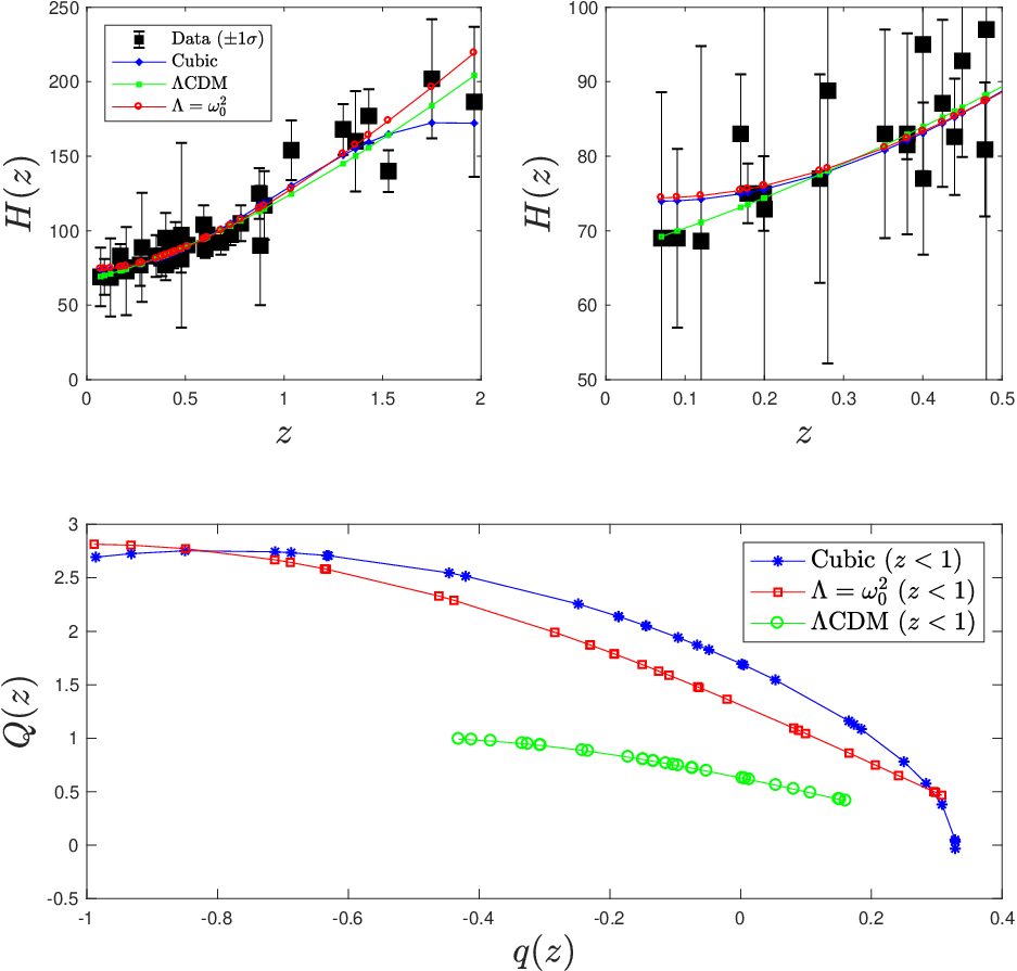
Table 1. Estimates of with uncertainties by nonlinear model regression applied
to the coefficients of the truncated Taylor series of cubic and quartic order, and to in
(10) with and (11) for CDM. is expressed in units of .
(Reprinted from [15].)
model
Cubic
-
-0.17
Quartic
-0.18
-0.18
CDM
0.5
Fig. 1 and Table 1 show a three-fold consistency among model-independent cubic and quartic fits and the model fit to (10). By cubic fit, CDM is inconsistent with data at .
Here, (12) is representative a near-extremal value of today. The associated relatively high estimate of from the cosmological data is free of tension with km s-1Mpc-1 obtained from surveys of the Local Universe, providing quantitative support for a dynamic dark energy (8). Combining results on , we estimate (15)
| (12) |
3 Asymptotic behavior in weak gravity
Applying (8) to (9) yields a second order differential equation, we have
| (13) |
associated with and and , defined by between dark pressure and dark energy. In the matter dominated era holds true in both (1) and (13), (8). In late time cosmology , however, is twice the value (1) of CDM, signifying fast evolution of the Hubble parameter .
The asymptotic regime of weak gravity satisfies the baryonic Tully-Fisher relation (Tully & Fisher, 1977) or, equivalently, Milgrom’s law (Milgrom, 1983),
| (14) |
In a background cosmology with dark energy (8), we have (15)
| (15) |
By (6), (15) introduces a sensitivity of galaxy dynamics in the regime (14) to the cosmological parameters , in addition to sensitivity to at the onset to weak gravity (). A recent sample of galaxy rotation curves at intermediate redshifts clusters close to the onset but is in the weak gravity regime (3). The transition to (14) is described by holographic inertia, sensitive to background parameters . By (10), this theory accounts for rotation curves from (Fig. 1) up to (15).
In this process, we encounter a deceleration parameter m s-2 (Table 1) with implied value m s-2. In what follows, we consider the rate of decay to (14) in
| (16) |
by specific values of , where .
Canonical estimates m s-2 derive from fitting an interpolating function to rotation curve data such as Fig. 1 (McGaugh, 2012, e.g.). Commonly used is , satisfying , gives
| (17) |
showing in (16).
Our value m s-2 is defined by the asymptotic value of in (18) in the notation of (15),
| (18) |
defined as a thermal average of the ratio of dispersion relations on the cosmological horizon and 3+1 spacetime within over momentum space as a function of , , whereby in terms of above. With , , , we have
| (19) |
where
| (20) |
In a confrontation with data as shown in Fig. 1, we face the fact that remains finite. In comparing from a fit using an interpolation function with associated with (15), discrepancies are expected by distinct decays and in (16). A fit to a tail of data of Fig. 1 involves the first two terms of (17), whereas (14) is attained to order in the latter. Writing , and satisfy
| (21) |
With , we conclude that under-estimates by
| (22) |
Indeed, a canonical value m s-2 obtains by fitting the full expression (17) to the data of Fig. 1, whereas a fit of the asymptotic relation (14) restricted to the tail gives
| (23) |
larger than by about 19%, as expected based on (22).
Our value m s-2, obtained from (15) based on estimating the cosmological parameters in Table 1, agrees with (23) to within about 17%, which is within the (statistical and systematic) uncertainties of about 20% in rotation curve data (Lelli et al., 2016, e.g.).
4 Conclusions and outlook
The tension problem points to a discrepancy between accelerated expansion and relatively stiff evolution in CDM. We here present a dynamical dark energy based on a fundamental frequency of the cosmological horizon, that is inherently positive and small. It introduces relatively fast evolution in the Hubble parameter today, satisfying with larger than that expected in CDM. A detailed confrontation with Hubble data covering an extended range in redshifts obtains an estimate of (Table 1) in full agreement with obtained from surveys of the Local Universe. Since (10-11) share the same parameters characterizing late time cosmology, dynamical dark energy and static dark energy can, for the first time, be simultaneously compared with data. The results of Table 1 favor the first and disfavor the second by .
Fast evolution (10) arises from novel behavior in the deceleration parameter , that changes the Hamiltonian energy constraint (9) to an ordinary differential equation which is second order in time, rather than first order in time in CDM. As such, (10) is a singular perturbation, disconnected from CDM. On this background, inertia of holographic origin is coevolving in the regime of weak gravity (3) with a specific predictions for anomalous behavior in galaxy dynamics, whose asymptotic behavior parameterized by (15) explicitly expresses sensitivity to background cosmology.
Results on (15) derived from fitting (10) to cosmological data on the Hubble parameter and derived from a direct fit to rotation curve data (Fig. 1) are consistent with rotation curve data within uncertainties. Our estimates of are slightly higher than canonical estimates, that we identify with a relatively fast decay of (18) in our theory of weak gravity to the asymptotic behavior (14).
Conceivably, conditions of weak gravity might be reproduced in laboratory (or satellite) experiments. While we cannot escape the presence of the gravitational field of the Earth (or the Sun), perhaps measurements on acceleration along equipotential surfaces in the gravitational field of the Earth (or the Sun) can be realized to test for anomalies , by observing geodesic separation between particles in free fall, as an extension of Galileo’s experiment. Suitable accelerations below may be imparted by gravitational or electrostatic forces.
Acknowledgements. This research is supported in part by the National Research Foundation of Korea (No. 2015R1D1A1A01059793 and 2016R1A5A1013277).
References
- Farooq et al. (2017) Farooq, O., Madiyar, F.R., Crandall, S., & Ratra, B., ApJ, 835, 26 (2017)
- Feynman (2003) Feynman, R.P., Morimigo, F.B., & Wagner, W.G., Feynman Lectures on Gravitation (Westview Press, Colorado, 2003), §7.1-2
- (3) Freedman, W.L., Nature Astronomy, 1, 0121 (2017)
- Lelli et al. (2016) Lelli, F., McGaugh, S.S., & Schombert, J.M., 2016, Astron. J., 152, 157
- Lelli et al. (2017) Lelli, F., McGaugh, S.S., Schombert, J.M., & Pawlowski, M.S., 2017, ApJ, 836, 152
- McGaugh (2012) McGaugh, S.S., 2012, ApJ, 143, 40
- Milgrom (1983) Milgrom, M., 1983, ApJ 270, 365
- Milgrom (1999) Milgrom, 1999, M., Phys. Lett. A 253, 273
- Smolin (2017) Smolin, L., 2017, arXiv:1704.00780
- Solá et al. (2017) Solà, J., Gómez-Valent, A., & de Cruz Pérez, J., 2017, ApJ, 836, 43
- Tully & Fisher (1977) Tully, R.B., & Fisher, J.R., 1977, Astron. Astrophys. 54, 661
- (12) van Putten, M.H.P.M., MNRAS 405, L48 (2015)
- (13) van Putten, M.H.P.M., ApJ 837, 22 (2017a)
- (14) van Putten, M.H.P.M., MPLA 32, 1730019 (2017b)
- (15) van Putten, M.H.P.M., ApJ, to appear (2017c)