Designing Quantum Information Processing via Structural Physical Approximation

We first recall that separable states are those quantum states that can be prepared by LOCC. They can be written in general as follows,

Separable states can be obtained by locally preparing $\rho_{i}^{(A)}$ and $\rho_{i}^{(B)}$ and communicating the probabilities $\{p_{i}\}$. An important property is the convexity. Separable states form a convex set: a probabilistic mixture of separable states is also separable. In mathematical terms, separable states are the dual to positive maps in a operator space. That is, those positive operators that remain positive under all positive maps are characterized as separable states. We write separable states as, denoted by $\mathrm{SEP}$

for all positive maps $\Lambda$.

Entangled states are those quantum states that cannot be prepared by LOCC, not possible to be written in the form of Eq. (7). They do not form a convex set: a mixture of entangled states can be a separable state. Note also that the set of bipartite quantum states is the dual to the CP maps $\mathrm{id}\otimes\Lambda\geq 0$, i.e.

Then, entangled states denoted by $\mathrm{ENT}$ corresponds to the complement to separable states, $\mathrm{ENT}=Q\setminus\mathrm{SEP}$. This shows that positive but not CP maps give the characterization as the dual to entangled states. In fact, all entangled states can be detected by positive but non-CP maps [28].

When it is found given systems are in an entangled states, the next is quantification of entanglement. We recall that LOCC is the operational task that can prepare only separable states but entangled ones, i.e., LOCC does not generate entanglement. An entanglement measure $E$ therefore has to fulfull the following constraints

Since LOCC does not increase entanglement, for states $\rho$ and $\sigma$ the measure $E$ satisfies the following property,

where $\rightarrow_{\mathrm{LOCC}}$ denotes an LOCC protocol transforming state $\rho$ to $\sigma$. It is clear that $\sigma$ is not more entangled than $\rho$. Then, it follows that

meaning that $\rho$ and $\sigma$ are equally entangled, or that they are equivalent up to local unitaries: there exist local unitaries $U=U^{(A)}\otimes U^{(B)}$ such that $U\rho U^{\dagger}=\sigma$.

The relation in Eq. (9) immediately shows that LOCC gives an order relation among quantum states. In fact, the set of bipartite states is totally ordered under LOCC, i.e. for any pair of states $\rho$ and $\sigma$, either $\rho\rightarrow_{\mathrm{LOCC}}\sigma$ or $\sigma\rightarrow_{\mathrm{LOCC}}\rho$ holds true. For states $\rho$, $\sigma$, and $\gamma$, we also have

Moreover, there is a unique root state in the order structure up to local unitaries such that all other states can be prepared by LOCC. The root state must be more entangled than any other states, for which it is called maximally entangled, and is given by in $S(\mathcal{H}_{d}\otimes\mathcal{H}_{d})$

We remark that the maximally entangled state can be identified only with the order relation with LOCC. A function of multipartite quantum states is called an entanglement monotone [50] if it satisfies the conditions in Eqs. (8) and (9), see also computable entanglement measures in Refs. [51, 52, 52, 53, 54, 55, 56, 57, 58]

Entangled states can be characterized by positive maps or, equivalently, entanglement witnesses (EWs). Both can detect entangled states. Entanglement detection is of both theoretical and practical importance as the characterization of entangled or separable states is highly non-trivial and entanglement is generally a useful resource for quantum information processing. When positive maps are attempted to apply to decide if given states are entangled or separable, one has to first completely identify given quantum states beforehand, with quantum state tomography. On the other hand, by applying EWs, entanglement can be detected even before learning given states with tomography.

In what follows, we show details of two aforementioned approaches of entanglement detection. We here restrict the consideration to single-copy level measurement, that is feasible with current technologies. Note that there are more efficient approaches that applies collective measurement on milti-copies, e.g. [59, 60]. Collective measurement is in general experimentally challenging as quantum memory is required to store quantum states for a while.

We first recall that positive but non-CP maps give the characterization of entangled states, vice versa. The condition that a map $\Lambda$ is positive but not CP can be rephrased by the followings,

Equivalently, a state $\rho$ is entangled if and only if there exists a positive but non-CP map $\Lambda$,

Entangled states can be identified by positive but not-CP maps. Note that, however, it has been a longstanding open problem in the context of operator algebra to have a complete characterization of positive but non-CP maps. Alternatively, it is also one of major challenging problems in quantum information theory to characterize separable states. This is referred to as the separability problem, which turns out to be in the NP-hard class [61].

Despite the fact that the decision problem itself is intractable, there have been fruitful directions with known examples of positive but non-CP maps. The first instance is the transpose operation, denoted by $T$,

The operation $\mathrm{id}\otimes T$ is called partial transpose and written as $\Gamma$. For state $\rho\in S(\mathcal{H}^{(A)}\otimes\mathcal{H}^{(B)})$, if it is found that $(\mathrm{id}\otimes T)[\rho]\ngeq 0$, one can conclude that the state is entangled [62]. The converse does not hold true in general: that is, there exist entangled states that remain positive under the partial transpose [63].

In fact, the partial transpose gives a simple criteria of identifying useful quantum states. Let us write those quantum states remaining (non-)positive after the partial transpose by (N)PPT, as follows,

It is clear that $\mathrm{SEP}\subset\mathrm{PPT}$. Note also that for $\mathrm{dim}(\mathcal{H}^{(A)})=2~\mathrm{and}~\mathrm{dim}(\mathcal{H}^{(B)})\in\{2,3\}$ we have that $\mathrm{SEP}=\mathrm{PPT}$ [62, 28]. There are entangled states which remain positive under the partial transpose, which are called PPT entangled states (PPTES). No entanglement can be distilled from PPTES. Note that for $\mathrm{dim}(\mathcal{H}^{(A)})=2~\mathrm{and}~\mathrm{dim}(\mathcal{H}^{(B)})\in\{2,3\}$, a positive map $\Lambda$ has a canonical form that

for some CP maps $\Lambda_{1}$ and $\Lambda_{2}$. In general, a positive map that can be written as the form in Eq. (12) is called decomposable.

An instance of decomposable maps is the reduction map, $\Lambda_{R}:S(\mathcal{H})\rightarrow S(\mathcal{H})$,

Then, the map $\mathrm{id}\otimes\Lambda_{R}$ is particularly useful as a distillability criteria [64]. If a state is detected by the reduction map, i.e., $[\mathrm{id}\otimes\Lambda_{R}](\rho)\ngeq 0$, then it is not only entangled but also distillable. Note that decomposable maps can detect only NPPT states.

Positive maps that are not in the form in Eq. (12) are called indecomposble, and can detect PPTES. A well-known example is Choi’s map, $\Lambda_{C}:S(\mathcal{H}_{3})\rightarrow S(\mathcal{H}_{3})$,

where the $|i-1\rangle=|i-1~\mathrm{mod}~3~\rangle$. That is, the map $\mathrm{id}\otimes\Lambda_{C}$ is not positive for some PPTES.

EWs that can detect entanglement of unknown states, i.e., even before verification of quantum states, can be constructed as follows. Let us restate the condition in Eq. (11): a state $\rho$ is entangled if and only if there exists a positive but non-CP map $\Lambda$ such that $[\mathrm{id}\otimes\Lambda](\rho)\ngeq 0$. This means that there exists a projector $Q\geq 0$ such that

that is, $Q$ is one of the projectors onto the subspace in which $(\mathrm{id}\otimes\Lambda)[\rho]$ contain negative eigenvalues. Note that there exists a dual map $\Lambda^{\dagger}$ such that the following holds true

Let us write by $W=(\mathrm{id}\otimes\Lambda^{\dagger})[Q]$ so that the right-hand-side can be written as $\mathrm{tr}[\rho W]$. Note also that the operator $W$ is Hermitian, $W=W^{\dagger}$.

In Eq. (14), suppose that $\rho$ is separable,. Then, the left-hand-side is positive since $\Lambda$ is positive and $Q\geq 0$. Thus, we have $\mathrm{tr}[\rho W]\geq 0$ for all separable states $\rho$. When $\rho$ is entangled, then there exists a map $\Lambda$ and $Q\geq 0$ such that the left-hand-side is negative. Then, we have $\mathrm{tr}[\rho W]<0$ for some entangled states $\rho$. To summarize, we have

These Hermitian operators are called EWs since they distinguish some entangled states from all separable states [65, 66, 67].

Let $\Lambda:\mathcal{B}(\mathcal{H}^{(A)})\rightarrow\mathcal{B}(\mathcal{H}^{(B)})$ denote a positive but non-CP map which does not correspond to a physical process. SPA to the map is given by,

where $p^{*}$ denotes the minimum $p$ that $\widetilde{\Lambda}$ is CP, and $d_{B}$ the dimension of Hilbert space $\mathcal{H}^{(B)}$. Note also that the depolarization map is denoted by $D_{A\rightarrow B}(\cdot)=\mathrm{I}/d_{B}$ with identity operator $\mathrm{I}$. The SPAed map $\widetilde{\Lambda}$ corresponds to a physical operation which can be implemented in experiment. Since the identity operator $\mathrm{I}$ is of full rank, there exists non-trivial $p^{*}\in(0,1)$ such that $\widetilde{\Lambda}$ is CP. The term, ”structural”, comes from the fact that the depolarization map $D_{A\rightarrow B}$ is admixed, which does not modify the structure of original map $\Lambda$ [29].

The construction of SPA can be generalized by considering more possibilities of CP maps in the place of depolarization map in Eq. (16) [68]. With a full-rank and normalized operator $K$, a generalization of SPA is given by

where $\mathcal{E}_{K}(\cdot)=K$. It is noteworthy that, to have a non-trivial $p_{K}^{*}\in(0,1)$, the operator $K$ should be of full-rank.

In general, SPA can be applied to non-positive maps $\mathrm{id}\otimes\Lambda$ which can detect entangled states as follows,

such that $\widetilde{\mathrm{id}\otimes\Lambda}\geq 0$ is CP, where $D_{i}(\cdot)=\mathrm{I}_{i}/d_{i}$ for $i=A,B$ denote the complete depolarization channel [30]. Note that $p^{*}$ is found as a minimal $p$ that the resulting map is CP.

The SPAed map in Eq. (17) can be applied to detecting entangled states as follows. Since $\rho\in S(\mathcal{H}^{(A)}\otimes\mathcal{H}^{(B)})$ is entangled if $(\mathrm{id}\otimes\Lambda)[\rho]\ngeq 0$ for some positive map $\Lambda\geq 0$, we have that $\rho$ is entangled if

The difference is that, whereas the map $\mathrm{id}\otimes\Lambda$ is not a physical process, SPAed map $\widetilde{\mathrm{id}\otimes\Lambda}$ corresponds to a quantum channel that can be experimentally realized. Therefore, the condition in Eq. (18) can be applied to entanglement detection in practice by incorporating to estimation of minimum eigenvalues. The scheme for entanglement detection has been proposed in Ref. [69] together with the spectrum estimation in Ref. [70]. The proposal is remarkable in that it directly applies positive maps to entanglement detection and also it provides an alternative approach to EWs.

Moreover, the SPAed map in Eq. (17) can be implemented by an LOCC protocol [71]. For the purpose, the inversion map has been introduced, $\Theta=-\mathrm{id}:S(\mathcal{H}^{(A)})\rightarrow S(\mathcal{H}^{(A)})$ and its SPA can be constructed as follows,

which is CP. Note that the inversion map is not even positive. Then, for a positive map $\Lambda:\mathcal{B}(\mathcal{H}^{(A)})\rightarrow\mathcal{B}(\mathcal{H}^{(B)})$, the LOCC scheme to realize SPA to the map $\mathrm{id}\otimes\Lambda$, see Eq. (17), can be found by the decomposition in the following,

where $P_{d_{A}}^{+}$ denotes the projection onto the $d_{A}$-dimensional maximally entangled state, see Eq. (10). The obtained decomposition shows that the map $\widetilde{\mathrm{id}\otimes\Lambda}$ can be implemented by performing local operations $\mathrm{id}\otimes\widetilde{\Lambda}$ and $\widetilde{\Theta}\otimes D_{A\rightarrow B}$ with probabilities $(1-q)$ and $q$, respectively. The LOCC scheme is useful when two parties far in distance implement the SPAed map and apply it to detecting entangled states.

Recall that positive maps and quantum states are closely related. One may observe how the relation between entanglement and positive maps evolves by SPA, by which positive maps are no longer non-CP and thus cannot detect entangled states. This has been elaborated and addressed as a conjecture that SPAed maps of optimal positive maps would characterize separable states [30]. For cases where the conjecture holds true, there is a huge simplification in implementation, namely that SPAed maps can be implemented via a measure-and-prepare protocol without entangled resources. This can also be applied to local operations in the SPAed map in Eq. (20).

In this subsection, we collect machineries to discuss relations between SPA and entanglement. The characterizations to positive maps, EWs, entangled states, separable states, and quantum channels, that have been discussed so far, can be viewed in a coherent way with the so-called Choi-Jamiołkowksi (CJ) isomorphisim [23, 24, 25]. It shows the one-to-one correspondence between the set of linear maps $\mathcal{B}(\mathcal{H}^{(A)})\rightarrow\mathcal{B}(\mathcal{H}^{(B)})$ and bipartite operators in $\mathcal{B}(\mathcal{H}^{(A)}\otimes\mathcal{H}^{(B)})$. By the isomorphism, a map $\Lambda:\mathcal{B}(\mathcal{H}^{(A)})\rightarrow\mathcal{B}(\mathcal{H}^{(A)})$ and a bipartite operator $\chi\in\mathcal{B}(\mathcal{H}^{(A)}\otimes\mathcal{H}^{(B)})$ are related as

where $P_{d_{A}}^{+}=|\phi_{d_{A}}^{+}\rangle\langle\phi_{d_{A}}^{+}|$ and $|\phi_{d_{A}}^{+}\rangle$ is the maximally entangled state in $S(\mathcal{H}_{A}\otimes\mathcal{H}_{A})$ in Eq. (10). We note that Eq. (21) shows that the linear map $\Lambda$ can be constructed from a given bipartite operator $\chi$ and conversely, Eq. (22) that the bipartite operator $\chi$ can be obtained from a linear map $\Lambda$. Throughout, let $\chi_{\Lambda}$ denote the CJ operator for a map $\Lambda$.

The CJ isomorphism is a useful tool in quantum information theory. It offers a unified view to the structure of positive maps and bipartite operators. Let us summarize the main results along the line, in the following.

1. 1.

   A linear map $\Lambda:S(\mathcal{H}^{(A)})\rightarrow S(\mathcal{H}^{(B)})$ is a quantum channel, i.e., CP and trace-preserving map, if and only if its CJ operator $\chi_{\Lambda}$ is a quantum state in $S(\mathcal{H}_{A}\otimes\mathcal{H}_{B})$, i.e., positive and of unit-trace. This means that all quantum states in $S(\mathcal{H}^{(A)}\otimes\mathcal{H}^{(B)})$ are obtained by sending the maximally entangled state $|\phi_{d_{A}}^{+}\rangle$ via a quantum channel $\mathrm{id}\otimes\Lambda$. Conversely, any quantum channel $\Lambda$ can be characterized by a quantum state $\chi$ as it is shown in Eq. (21).

   To see this explicitly, one can rewrite Eq. (21) as follows [72]

   $\displaystyle\Lambda[(\cdot)]=d_{A}^{2}~\mathrm{tr}_{A^{\prime}A}[(\cdot)_{A^{\prime}}^{T}\otimes\chi^{(AB)}~(|\phi_{d_{A}}^{+}\rangle_{A^{\prime}A}\langle\phi_{d_{A}}^{+}|)]$

   (23)

   where we have assumed that $d_{A^{\prime}}=d_{A}$. This can be interpreted as quantum teleportation of quantum state at location $A^{\prime}$ via shared entangled state $\chi^{(AB)}$ between $A$ and $B$, see also Fig. 3. Note that the factor $d_{A}^{2}$ amounts to the success probability of measurement on the basis $P_{d_{A}}^{+}$ ¹¹ 1 Bell-states used in two-qubit quantum teleportation can be generalized to high-dimensions with Weyl operators, $\mathcal{W}_{m,n}=\sum_{k}e^{\frac{2\pi i}{d}kn}|k\rangle\langle k+m|$ for $m,n=0,\cdots,d-1$, so that $|\Phi_{m,n}\rangle=(\mathrm{id}\otimes\mathcal{W}_{m,n})|\Phi_{d_{A}}^{+}\rangle$. .

2. 2.

   A linear map $\Lambda$ is positive but non-CP if and only if its CJ operator $\chi_{\Lambda}$ is an EW. That is, an EW can be obtained from a positive but non-CP map in general, as

   $\displaystyle W_{\Lambda}=(\mathrm{id}\otimes\Lambda)[P_{d_{A}}^{+}].$

   (24)

   EWs are called (in-)decomposable if positive maps $\Lambda$ are (in-)decomposable. PPTES are detected by indecomposable EWs [73].

The isomorphism between quantum channels and CJ operators shown in Eq. (23) is useful to characterize properties of quantum states and channels. Suppose that, for a quantum channel $\Lambda$, the corresponding quantum state $\chi_{\Lambda}=(\mathrm{id}\otimes\Lambda)[{P_{d_{A}}^{+}}]$ is separable and also that it has the following separable decomposition,

Note that if $[\mathrm{id}\otimes\Lambda]({P_{d_{A}}^{+}})$ is separable, states $[\mathrm{id}\otimes\Lambda](\rho)$ are also separable for any state $\rho$ [74]. A quantum channel $\Lambda$ is called entanglement-breaking if for all states $\rho\in S(\mathcal{H}^{(A)}\otimes\mathcal{H}^{(B)})$ the resulting states $(\mathrm{id}\otimes\Lambda)[\rho]$ are separable [74]. From the isomorphism in Eqs. (22) and (23), one can find the corresponding map in the following form

This shows that, for a given state, the channel works as preparation of quantum state $\{|f_{i}\rangle\langle f_{i}|\}_{i}$ followed by measurement outcomes with POVMs $\{p_{i}|e_{i}^{*}\rangle\langle e_{i}^{*}|\}_{i}$. That is, entanglement-breaking channels can be implemented by a measure-and-prepare scheme. Conversely, a measure-and-prepare channel with rank-one POVMs is entanglement-breaking.

It can happen that for a quantum channel $\Lambda$, its CJ operator is a bound entangled state [63]. The channel is called entanglement-binding. For instance, a channel $\Lambda$ is entanglement-binding if the CJ operator $\chi_{\Lambda}$ is PPTES. A quantum channel $\Lambda$ is called PPT-preserving if its CJ operator $\chi_{\Lambda}=(\mathrm{id}\otimes\Lambda){P_{d_{A}}^{+}}$ is PPT, i.e., $\chi_{\Lambda}^{T}\geq 0$.

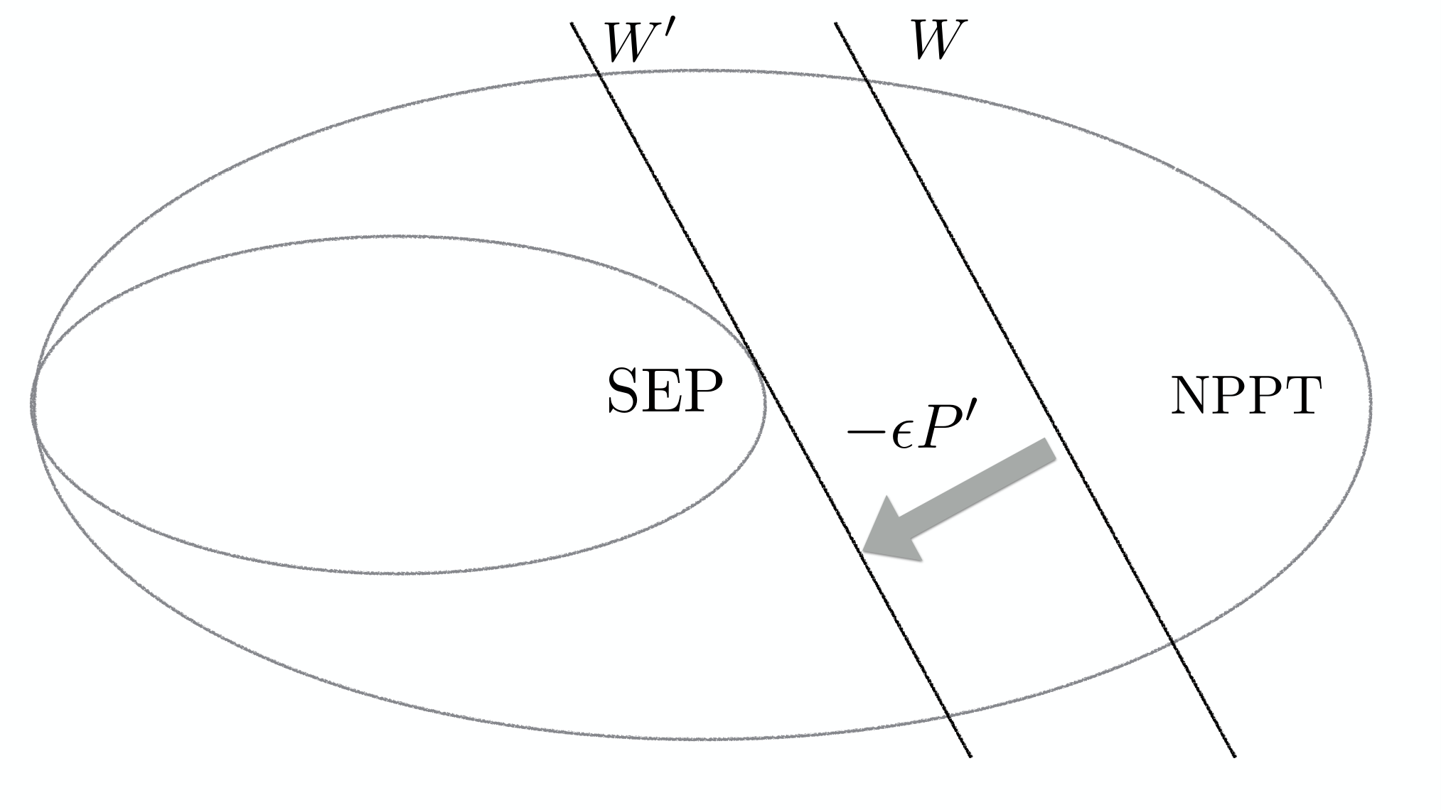
The isomorphism establishes the connection between positive but non-CP maps and EWs. In Eq. (24), a positive but non-CP map can be either decomposable or indecomposable, by which one can find a canonical form of EWs as follows,

If $P\geq 0$, the EW can detect NPPT states and is called a decomposable EW. For some NPPT state $\rho$, we have $\mathrm{tr}[\rho W]=\mathrm{tr}[\rho P]+\mathrm{tr}[\rho^{\Gamma}Q]$, which is negative if $-\mathrm{tr}[\rho^{\Gamma}Q]>\mathrm{tr}[\rho P]\geq 0$.

Two EWs $W_{i}=P_{i}+Q^{\Gamma}$ for $i=1,2$ with $P_{1}\geq P_{2}$ can be compared in terms of the detection capability [73]. Denoted the set of detected states by $W$ as

one can find that $D_{W_{1}}\subset D_{W_{2}}$. That is, all states detected by $W_{1}$ are also detected by $W_{2}$. Then, $W_{2}$ is called finer than $W_{1}$. When an EW is finer than any other EWs, it is called optimal [73]. When an EW is not optimal, optimization can be performed by subtracting positive operators: $W_{1}\rightarrow W^{\prime}=W_{1}-\epsilon P^{\prime}$ for some $P^{\prime}\geq 0$ and $\epsilon\geq 0$. Then, EW $W$ is optimal if for any $P^{\prime}\geq 0$ and arbitrary $\epsilon>0$, $W-\epsilon P^{\prime}$ is no longer an EW. Collecting optimal EWs, all entangled states can be detected.

It is not immediate to find optimality of EWs. A useful method is the so-called spanning property, that is only sufficient condition for optimal EWs. Let $P_{W}$ denote the set of product states on which a witness $W$ vanishes,

We call $W$ contains the spanning property if $P_{W}$ can span the whole space, i.e., $\mathrm{span}~{P_{W}}=\mathcal{H}^{(A)}\otimes\mathcal{H}^{(B)}$. If an EW contains the spanning property, it is optimal. The converse, however, does not hold true in general.

In Eq. (26), EWs are called indecomposable if they are obtained from indecomposable positive maps. In this case, we have $P\ngeq 0$ in Eq. (26) and EWs can detect PPTES. Similarly, the optimization process works by subtracting decomposable operators, that are in the following form in general $D=P^{\prime}+Q^{\prime\Gamma}$ with $P^{{}^{\prime}},Q^{{}^{\prime}}\geq 0$. When there is no decomposable operator that can be subtracted, the resulting EWs are called non-decomposable-optimal. I.e., $W$ is non-decomposable optimal if $\forall\epsilon>0$ and for all decomposable operators $D$, it holds that $W-\epsilon D$ is no longer an EW [73].

Then, from Eq. (21) positive maps can be obtained from EWs, i.e. given $W$, the positive map can be derived as $\Lambda(\cdot)=d_{A}\mathrm{tr}[W((\cdot)^{T}\otimes\mathrm{I})]$. Positive maps are called (indecomposable) optimal if they are derived from (indecomposable) optimal EWs. EWs have been a useful tool to investigate various structures and properties of entangled states. More properties and structures of EWs, such as optimality, extremality, atomicity, etc. have been explained in a recent review [67].

In this subsection, we discuss the relation between SPA and quantum channels, namely the conjecture addressed in Ref. [30] that SPAed maps to optimal positive maps correspond to entanglement-breaking channels. While there have been a number of supporting examples [30, 31, 32, 33, 34, 35, 36], counterexamples have been finally found, firstly in indecomposable cases [37, 38] and then decomposable cases [39], see also numerical evidences [75] and a recent review [46]. In the following, we address the conjecture with an observation on no-go theorems in quantum theory and overview the progress. Positive maps that satisfy the conjecture are considered in detail and their practical applications are shown in the next section.

An observation on no-go theorems. The conjecture has been motivated by an attempt to understanding disallowed dynamics in quantum theory. For instance, the no-cloning theorem states that unkonwn quantum states cannot be perfectly copied [17, 76], which is closely related to the other, the impossibility of perfect state discrimination [77, 78, 79, 80, 81, 82, 83, 84]. Note that the no-go theorems are the key elements in some of quantum information applications, e.g. quantum cryptographic protocols [85, 22].

We now observe quantum operations that make approximations to disallowed dynamics, as follows. One can firstly consider optimal quantum cloning, for instance, the symmetric and universal $1\rightarrow 2$ cloning operation [86]. It is clear that the $1\rightarrow 2$ quantum cloning is not an entangling-breaking channel. However, asymptotic quantum cloning where output clones tend to be sufficiently large, i.e., $N\rightarrow\infty$ quantum cloning, converges to entanglement-breaking [20, 21]. Application of asymptotic quantum cloning to bipartite quantum states gets rid of entangled states.

One can also consider another impossible operational task having different origin of the impossibility in quantum theory. Arbitrary manipulation of unknown quantum states is generally disallowed [87], among which the universal-NOT (UNOT) operation is an extreme case [88, 89, 90] and not possible either. The ideal UNOT operation works as

i.e., converting a state to its orthogonal complement. This is, however, an anti-unitary transformation that does not preserve a physical symmetry and consequently cannot be a legitimate quantum operation [91]. In Ref. [88], a quantum channel that optimally approximates the UNOT operation has been shown. It turns out that the resulting quantum operation can be implemented by a measure-and-prepare protocol, that corresponds to an entanglement-breaking channel. We emphasize that the best approximate quantum operation turns out to be entanglement-breaking.

It is worth noting that the ideal UNOT operation is a positive but non-CP map since it can be rewritten as, from Eq. (27),

with the transpose map $T$ and Pauli matrix $Y$. This shows that the UNOT is equivalent to the transpose map up to a local unitary transformation. This immediately implies that for qubit states, SPA to the transpose is a measure-and-prepare scheme, that is, entanglement-breaking. This holds true in continuous-variable systems [92].

The result in Ref. [90] is particularly interesting. It shows that the optimal approximate UNOT coincides to what appears in the ancilla of the $1\rightarrow 2$ quantum cloning [86]. To be precise, we note that the $1\rightarrow 2$ quantum cloning produces three qubits, in which two are approximate clones and the other is ancilla. The process happened in the ancila is named quantum anti-cloning, that coincides to an optimal approximate UNOT. In Ref. [93], the approximate UNOT has been experimentally realized via the aforementioned anti-cloning process by implementing the $1\rightarrow 2$ quantum cloning. Technically, the approximating UNOT corresponds to the complementary channel of the $1\rightarrow 2$ quantum cloning. Recall that the approximate UNOT operation is entanglement-breaking and can be equivalently implemented by a measure-and-prepare scheme [41].

The conjecture. It has been observed that the approximate UNOT corresponds to an entanglement-breaking channel, by which all quantum states are mapped to separable states. From the fact that entanglement is closely connected to disallowed dynamics, UNOT, quantum cloning, the transpose map, etc., one may understand that approximations to the impossible tasks would be necessarily entanglement-breaking which gets rid of entangled states.

In fact, from Eq. (16) the SPAed transpose can be written as $\widetilde{T}=T\circ D_{p^{*}}$ where $D_{p}(\rho)=(1-p^{*})\rho+(p^{*}/d)\mathrm{I}$ is an entanglement-breaking channel. The decomposition may elucidate the mathematical structure that the CP map $\widetilde{T}$ works by applying the transpose $T$ to separable states after the entanglement-breaking channel $D_{p^{*}}$, see Fig. 5. See also that the decomposition is referred to as $\mathrm{Positive}$-divisible map after properly including a parameter indicating time-evolution [94, 95]. In the range of the depolarization $D_{p^{*}}$, there are only separable states for which positive but non-CP maps have no reason to be regarded as non-physical ones. It can also be interpreted that, therefore, SPA to optimal positive maps should necessarily get rid of entangled states, hence, entanglement-breaking. The SPA conjecture generalizes the observation and has been addressed as follows [30].

SPAs to optimal positive maps correspond to entanglement-breaking channels. Equivalently, SPAed optimal EWs are separable states.

The conjecture can be tested in the following way. For a optimal positive map $\Lambda$, one has to firstly find the SPAed map $\widetilde{\Lambda}$ with $p^{*}$, see Eq. (16). This can be obtained by finding minimal $p^{*}$ such that $(\rm{id}\otimes\Lambda)[P_{d}^{+}]\geq 0$ [74, 30]. The non-trivial part is to check if the map $\widetilde{\Lambda}$ is entanglement-breaking or not. To do this, one has to determine if its CJ state $(\rm{id}\otimes\Lambda)[P_{d}^{+}]$ is separable, or not. If it is separable, it implies that the SPAed map is entanglement-breaking. Otherwise, the conjecture is disproven.

Note that by admixing sufficient noise a non-CP map can always transformed to a CP map [68]. Let $p_{s}$ denote the noise parameter in Eq. (16) instead of $p^{*}$ such that the resulting CP map is entanglement-breaking. It holds that $p_{s}\geq p^{*}$ in general, and the conjecture addresses the question if the equality holds for all optimal positive maps.

Interestingly, there have been numerous examples of positive maps that support the conjecture [30, 31, 32, 33, 34, 35, 36]. Recall that once a quantum channel is entanglement-breaking, there is a huge simplification in implementation that it can be performed by a measure-and-prepare scheme. Then, a quantum channel is designed as measurement of an input state and preparation of a quantum state according to measurement outcomes. In the next section 5, structures of SPAed maps for positive maps satisfying the conjecture are shown and the detailed derivations are presented.

Among the examples, a general property has been shown in Refs. [32, 68]. Note that the class of isotropic states is given by $\rho_{\mathrm{iso}}=(1-p)P_{d}^{+}+(p/d^{2})\mathrm{I}$, which is NPPT entangled when $p\in[0,d/(d+1))$ and otherwise separable.

Theorem. If a positive map $\Lambda:\mathcal{B}(\mathcal{H}_{d})\rightarrow\mathcal{B}(\mathcal{H}_{d})$ detects all entangled isotropic states in the dimension, then its SPAed map $\widetilde{\Lambda}$ is entanglement-breaking.

This is useful when testing if a positive map satisfies the conjecture. In fact, it can be applied to the transpose, Reduction map, and some of Breuer-Hall maps [30]. Note that Choi’s map in Eq. (13) also satisfies the conjecture. We also remark that, interestingly, in the theorem above the optimality of positive maps is not necessary to fulfill the conjecture.

The conjecture has been extended to continuous-variable systems, and specially considered for Gaussian states [96]. In this case, the transpose map is particularly interesting since almost all entangled Gaussian states are NPPT, i.e., by the partial transpose significant fractions of entangled Gaussian states can be detected. The transpose map, denoted by $T_{G}$, works on the level of displacement operators [97, 98]. In Ref. [68], it has been shown that the SPAed Gaussian channel $\widetilde{T}_{G}$ is entanglement-breaking, namely measurement in and preparation of coherent states, i.e.,

where $|x,y\rangle$ denotes a coherent state having displacements in $x$ and $y$.

Finally, the conjecture is disproven for both indecomposable [37, 38] and decomposable cases [39], see also numerical evidences [75]. We also refer to the excellent reviews on the mathematical structure of the conjecture and the counterexamples [46] and on the detailed terms of optimality, extremality, atomicity, and facial structures of EWs [73, 67]. The counterexample for indecomposable cases is given in Ref. [99] that has been obtained by further generalizations of Choi maps in Ref. [100]. The map is given in $3$-dimensional Hilbert space: for non-negative real numbers $a$, $b$, and $c$ and $\theta\in[-\pi,\pi]$ and $X=(x_{i,j})\in M_{3}$,

With this example, the conjecture is tested and disproven in Ref. [37] where the conic properties of EWs have been completely analyzed. Namely, the SPAed map is not entanglement-breaking for $b>0$ and $\theta\in(-\pi/3,0)\cup(0,\pi/3)$.

Qubit states. We begin with the SPA to the transpose for qubit states and provide the derivation in detail. For qubit states, the transpose can be defined without dependence on the choice of basis. For convenience, let us take the transpose with respect to computational basis as follows,

Note that the transpose itself is a linear and positive map. The SPA to the transpose is then obtained from the construction in Eq. (16),

for which it holds that $\widetilde{T}$ is completely positive, i.e. $(\mathrm{id}\otimes\widetilde{T})(|\phi_{2}^{+}\rangle\langle\phi_{2}^{+}|)\geq 0$. Note that it is found $p^{*}=2/3$.

To realize the SPAed transpose $\widetilde{T}$ in a prepare-and-measure scheme, one can exploit the isomorphism between channels and states. Given the map $\widetilde{T}$, the CJ operator can be found as,

where $|\phi^{\pm}\rangle=(|00\rangle\pm|11\rangle)/\sqrt{2}$ and $|\psi^{\pm}\rangle=(|01\rangle\pm|10\rangle)/\sqrt{2}$. Note that the state in the above is separable [6].Then, from the isomorphism between states and channels, one can find the channel performing the SPA to the transpose as follows, see Eq. (23)

References

- [2] Shor P 1999 SIAM Review 41 303–332 URL http://dx.doi.org/10.1137/S0036144598347011
- [3] Grover L K 1996 A fast quantum mechanical algorithm for database search Proceedings of the Twenty-eighth Annual ACM Symposium on Theory of Computing STOC ’96 (New York, NY, USA: ACM) pp 212–219 ISBN 0-89791-785-5 URL http://doi.acm.org/10.1145/237814.237866
- [4] Zalka C 1999 Physical Review A 60 2746–2751 URL http://link.aps.org/doi/10.1103/PhysRevA.60.2746
- [5] Schrödinger E 1935 Mathematical Proceedings of the Cambridge Philosophical Society 31 555–563 URL https://www.cambridge.org/core/article/div-class-title-discussion-of-probability-relations-between-separated-systems-div/C1C71E1AA5BA56EBE6588AAACB9A222D
- [6] Werner R F 1989 Physical Review A 40 4277–4281 URL http://link.aps.org/doi/10.1103/PhysRevA.40.4277
- [7] Horodecki R, Horodecki P, Horodecki M and Horodecki K 2009 Rev. Mod. Phys. 81(2) 865–942 URL http://link.aps.org/doi/10.1103/RevModPhys.81.865
- [8] Raussendorf R and Briegel H J 2001 Physical Review Letters 86 5188–5191 URL http://link.aps.org/doi/10.1103/PhysRevLett.86.5188
- [9] Bennett C H, DiVincenzo D P, Smolin J A and Wootters W K 1996 Physical Review A 54 3824–3851 URL http://link.aps.org/doi/10.1103/PhysRevA.54.3824
- [10] Żukowski M, Zeilinger A, Horne M A and Ekert A K 1993 Physical Review Letters 71 4287–4290 URL http://link.aps.org/doi/10.1103/PhysRevLett.71.4287
- [11] Briegel H J, Dür W, Cirac J I and Zoller P 1998 Physical Review Letters 81 5932–5935 URL http://link.aps.org/doi/10.1103/PhysRevLett.81.5932
- [12] Curty M, Lewenstein M and Lütkenhaus N 2004 Physical Review Letters 92 217903– URL http://link.aps.org/doi/10.1103/PhysRevLett.92.217903
- [13] Acin A and Gisin N 2005 Physical Review Letters 94 020501– URL http://link.aps.org/doi/10.1103/PhysRevLett.94.020501
- [14] Gisin N and Wolf S 1999 Phys. Rev. Lett. 83(20) 4200–4203 URL http://link.aps.org/doi/10.1103/PhysRevLett.83.4200
- [15] Smith G and Yard J 2008 Science 321 1812 URL http://science.sciencemag.org/content/321/5897/1812.abstract
- [16] Palazuelos C 2012 Physical Review Letters 109 190401– URL http://link.aps.org/doi/10.1103/PhysRevLett.109.190401
- [17] Wootters W K and Zurek W H 1982 Nature 299 802–803 URL http://dx.doi.org/10.1038/299802a0
- [18] Gisin N 1998 Physics Letters A 242 1–3 URL http://www.sciencedirect.com/science/article/pii/S0375960198001704
- [19] Bruss D, Ekert A and Macchiavello C 1998 Physical Review Letters 81 2598–2601 URL http://link.aps.org/doi/10.1103/PhysRevLett.81.2598
- [20] Bae J and Acin A 2006 Physical Review Letters 97 030402– URL http://link.aps.org/doi/10.1103/PhysRevLett.97.030402
- [21] Chiribella G and D’Ariano G M 2006 Physical Review Letters 97 250503– URL http://link.aps.org/doi/10.1103/PhysRevLett.97.250503
- [22] Bennett C H 1992 Physical Review Letters 68 3121–3124 URL http://link.aps.org/doi/10.1103/PhysRevLett.68.3121
- [23] Pillis J d 1967 PACIFIC JOURNAL OF MATHEMATICS 23 129
- [24] Jamiołkowski A 1972 Reports on Mathematical Physics 3 275–278 URL http://www.sciencedirect.com/science/article/pii/0034487772900110
- [25] Choi M D 1975 Linear Algebra and its Applications 10 285–290 URL http://www.sciencedirect.com/science/article/pii/0024379575900750
- [26] Breuer H P 2007 Oxford Press
- [27] Woronowicz S L 1976 Reports on Mathematical Physics 10 165–183 URL http://www.sciencedirect.com/science/article/pii/0034487776900380
- [28] Horodecki M, Horodecki P and Horodecki R 1996 Physics Letters A 223 1–8 URL http://www.sciencedirect.com/science/article/pii/S0375960196007062
- [29] Horodecki P 2003 Physical Review A 68 052101– URL http://link.aps.org/doi/10.1103/PhysRevA.68.052101
- [30] Korbicz J K, Almeida M L, Bae J, Lewenstein M and Acin A 2008 Physical Review A 78 062105– URL http://link.aps.org/doi/10.1103/PhysRevA.78.062105
- [31] Chruściński D, Pytel J and Sarbicki G 2009 Physical Review A 80 062314– URL http://link.aps.org/doi/10.1103/PhysRevA.80.062314
- [32] Chruściński D and Pytel J 2010 Physical Review A 82 052310– URL http://link.aps.org/doi/10.1103/PhysRevA.82.052310
- [33] Chruściński D and Pytel J 2011 Journal of Physics A: Mathematical and Theoretical 44 165304 URL http://stacks.iop.org/1751-8121/44/i=16/a=165304
- [34] Zwolak J P and Chruściński D 2013 Reports on Mathematical Physics 71 163–175 URL http://www.sciencedirect.com/science/article/pii/S0034487713600270
- [35] Zwolak J P and Chruściński D 2014 Physical Review A 89 052314– URL http://link.aps.org/doi/10.1103/PhysRevA.89.052314
- [36] Augusiak R, Bae J, Tura J and Lewenstein M 2014 Journal of Physics A: Mathematical and Theoretical 47 065301 URL http://stacks.iop.org/1751-8121/47/i=6/a=065301
- [37] Ha K C and Kye S H 2012 Journal of Mathematical Physics 53 102204 URL http://scitation.aip.org/content/aip/journal/jmp/53/10/10.1063/1.4754279
- [38] Størmer E 2013 Journal of Functional Analysis 264 2197–2205 URL http://www.sciencedirect.com/science/article/pii/S0022123613000682
- [39] Chruściński D and Sarbicki G 2014 Journal of Physics A: Mathematical and Theoretical 47 195301 URL http://stacks.iop.org/1751-8121/47/i=19/a=195301
- [40] Hansen L O and Myrheim J 2015 Physical Review A 92 042306– URL http://link.aps.org/doi/10.1103/PhysRevA.92.042306
- [41] Lim H T, Ra Y S, Kim Y S, Bae J and Kim Y H 2011 Physical Review A 83 020301– URL http://link.aps.org/doi/10.1103/PhysRevA.83.020301
- [42] Lim H T, Kim Y S, Ra Y S, Bae J and Kim Y H 2011 Phys. Rev. Lett. 107(16) 160401 URL http://link.aps.org/doi/10.1103/PhysRevLett.107.160401
- [43] Lim H T, Kim Y S, Ra Y S, Bae J and Kim Y H 2012 Physical Review A 86 042334– URL http://link.aps.org/doi/10.1103/PhysRevA.86.042334
- [44] Kalev A and Bae J 2013 Physical Review A 87 062314– URL http://link.aps.org/doi/10.1103/PhysRevA.87.062314
- [45] Graydon M A and Appleby D M 2016 Journal of Physics A: Mathematical and Theoretical 49 33LT02 URL http://stacks.iop.org/1751-8121/49/i=33/a=33LT02
- [46] Shultz F 2016 Journal of Mathematical Physics 57 015218 URL http://scitation.aip.org/content/aip/journal/jmp/57/1/10.1063/1.4938226;jsessionid=XkLDevjM9fvkF1kO3FB1TlMe.x-aip-live-03
- [47] Gleason A 1957 Indiana Univ. Math. J. 6 885
- [48] Stinespring W F 1955 6 211–216 URL http://www.jstor.org/stable/2032342
- [49] Kraus K 1983 States, Effects, and Operations Fundamental Notions of Quantum Theory (Springer)
- [50] Vidal G 2000 Journal of Modern Optics 47 355–376 URL http://www.tandfonline.com/doi/abs/10.1080/09500340008244048
- [51] Wootters W K 1998 Physical Review Letters 80 2245–2248 URL http://link.aps.org/doi/10.1103/PhysRevLett.80.2245
- [52] Vollbrecht K G H and Werner R F 2001 Physical Review A 64 062307– URL http://link.aps.org/doi/10.1103/PhysRevA.64.062307
- [53] Terhal B M and Vollbrecht K G H 2000 Physical Review Letters 85 2625–2628 URL http://link.aps.org/doi/10.1103/PhysRevLett.85.2625
- [54] Mintert F, Kuś M and Buchleitner A 2004 Physical Review Letters 92 167902– URL http://link.aps.org/doi/10.1103/PhysRevLett.92.167902
- [55] Mintert F, Carvalho A R, Kuś M and Buchleitner A 2005 Physics Reports 415 207–259 URL http://www.sciencedirect.com/science/article/pii/S0370157305002334
- [56] Mintert F and Buchleitner A 2005 Physical Review A 72 012336– URL http://link.aps.org/doi/10.1103/PhysRevA.72.012336
- [57] Mintert F 2007 Applied Physics B 89 493–497 URL http://dx.doi.org/10.1007/s00340-007-2864-7
- [58] Bae J, Tiersch M, Sauer S, de Melo F, Mintert F, Hiesmayr B and Buchleitner A 2009 Physical Review A 80 022317– URL http://link.aps.org/doi/10.1103/PhysRevA.80.022317
- [59] Augusiak R, Demianowicz M and Horodecki P 2008 Physical Review A 77 030301– URL http://link.aps.org/doi/10.1103/PhysRevA.77.030301
- [60] Mintert F and Buchleitner A 2007 Physical Review Letters 98 140505– URL http://link.aps.org/doi/10.1103/PhysRevLett.98.140505
- [61] Gurvits L 2004 J. Comput. Syst. Sci. 69 448–484 ISSN 0022-0000 URL http://dx.doi.org/10.1016/j.jcss.2004.06.003
- [62] Peres A 1996 Physical Review Letters 77 1413–1415 URL http://link.aps.org/doi/10.1103/PhysRevLett.77.1413
- [63] Horodecki P, Horodecki M and Horodecki R 1999 Physical Review Letters 82 1056–1059 URL http://link.aps.org/doi/10.1103/PhysRevLett.82.1056
- [64] Horodecki M and Horodecki P 1999 Physical Review A 59 4206–4216 URL http://link.aps.org/doi/10.1103/PhysRevA.59.4206
- [65] Terhal B M 2000 Physics Letters A 271 319–326 URL //www.sciencedirect.com/science/article/pii/S0375960100004011
- [66] Gühne O and Tóth G 2009 Physics Reports 474 1–75 URL //www.sciencedirect.com/science/article/pii/S0370157309000623
- [67] Chruściński D and Sarbicki G 2014 Journal of Physics A: Mathematical and Theoretical 47 483001 URL http://stacks.iop.org/1751-8121/47/i=48/a=483001
- [68] Augusiak R, Bae J, ŁCzekaj and Lewenstein M 2011 Journal of Physics A: Mathematical and Theoretical 44 185308 URL http://stacks.iop.org/1751-8121/44/i=18/a=185308
- [69] Horodecki P and Ekert A 2002 Physical Review Letters 89 127902– URL http://link.aps.org/doi/10.1103/PhysRevLett.89.127902
- [70] Keyl M and Werner R F 2001 Physical Review A 64 052311– URL http://link.aps.org/doi/10.1103/PhysRevA.64.052311
- [71] Alves C M, Horodecki P, Oi D K L, Kwek L C and Ekert A K 2003 Physical Review A 68 032306– URL http://link.aps.org/doi/10.1103/PhysRevA.68.032306
- [72] Cirac J I, Dür W, Kraus B and Lewenstein M 2001 Physical Review Letters 86 544–547 URL http://link.aps.org/doi/10.1103/PhysRevLett.86.544
- [73] Lewenstein M, Kraus B, Cirac J I and Horodecki P 2000 Physical Review A 62 052310– URL http://link.aps.org/doi/10.1103/PhysRevA.62.052310
- [74] Horodecki M, Shor P W and Ruskai M B 2003 Reviews in Mathematical Physics 15 629–641 URL http://dx.doi.org/10.1142/S0129055X03001709
- [75] Hansen L O, Hauge A, Myrheim J and Sollid P Ø 2015 International Journal of Quantum Information 13 1550060 URL http://dx.doi.org/10.1142/S0219749915500604
- [76] Scarani V, Iblisdir S, Gisin N and Acin A 2005 Reviews of Modern Physics 77 1225–1256 URL http://link.aps.org/doi/10.1103/RevModPhys.77.1225
- [77] Helstrom C W 1976 Quantum detection and estimation theory (Academic Press)
- [78] Holevo A S 1974 Remarks on optimal quantum measurements vol 10 (Problemy Peredachi Informacii)
- [79] Yuen H, Kennedy R and Lax M 1975 IEEE Transactions on Information Theory 21 125–134
- [80] Chefles A 2000 Contemporary Physics 41 401–424 URL http://dx.doi.org/10.1080/00107510010002599
- [81] Bergou J A, Herzog U and Hillery M 2004 11 Discrimination of Quantum States (Berlin, Heidelberg: Springer Berlin Heidelberg) pp 417–465 ISBN 978-3-540-44481-7
- [82] Bergou J A 2007 Quantum state discrimination and selected applications vol 84 (Journal of Physics: Conference Series)
- [83] Barnett S M and Croke S 2009 Advances in Optics and Photonics 1 238–278 URL http://aop.osa.org/abstract.cfm?URI=aop-1-2-238
- [84] Bae J and Kwek L C 2015 Journal of Physics A: Mathematical and Theoretical 48 083001 URL http://stacks.iop.org/1751-8121/48/i=8/a=083001
- [85] Bennett C H and Brassard G IEEE, New York, 1984 Proceedings of IEEE International Conference on Computers, Systems, and Signal Processing, Bangalore, India 175 8
- [86] Buzek V and Hillery M 1996 Physical Review A 54 1844–1852 URL http://link.aps.org/doi/10.1103/PhysRevA.54.1844
- [87] Hardy L and Song D D 2001 Physical Review A 63 032304– URL http://link.aps.org/doi/10.1103/PhysRevA.63.032304
- [88] Buzek V, Hillery M and Werner R F 1999 Physical Review A 60 R2626–R2629 URL http://link.aps.org/doi/10.1103/PhysRevA.60.R2626
- [89] Gisin N and Popescu S 1999 Physical Review Letters 83 432–435 URL http://link.aps.org/doi/10.1103/PhysRevLett.83.432
- [90] Bechmann-Pasquinucci H and Gisin N 1999 Physical Review A 59 4238–4248 URL http://link.aps.org/doi/10.1103/PhysRevA.59.4238
- [91] Wigner E P 1960 Journal of Mathematical Physics 1 409–413 URL http://scitation.aip.org/content/aip/journal/jmp/1/5/10.1063/1.1703672
- [92] Buscemi F, D’Ariano G M, Perinotti P and Sacchi M F 2003 Physics Letters A 314 374–379 URL http://www.sciencedirect.com/science/article/pii/S037596010300954X
- [93] De Martini F, Buzek V, Sciarrino F and Sias C 2002 Nature 419 815–818 URL http://dx.doi.org/10.1038/nature01093
- [94] Chruściński D and Maniscalco S 2014 Physical Review Letters 112 120404– URL http://link.aps.org/doi/10.1103/PhysRevLett.112.120404
- [95] Breuer H P, Laine E M and Piilo J 2009 Physical Review Letters 103 210401– URL http://link.aps.org/doi/10.1103/PhysRevLett.103.210401
- [96] Horodecki P and Lewenstein M 2000 Physical Review Letters 85 2657–2660 URL http://link.aps.org/doi/10.1103/PhysRevLett.85.2657
- [97] Simon R 2000 Phys. Rev. Lett. 84(12) 2726–2729 URL http://link.aps.org/doi/10.1103/PhysRevLett.84.2726
- [98] Duan L M, Giedke G, Cirac J I and Zoller P 2000 Physical Review Letters 84 2722–2725 URL http://link.aps.org/doi/10.1103/PhysRevLett.84.2722
- [99] Ha K C and Kye S H 2012 Journal of Physics A: Mathematical and Theoretical 45 415305 URL http://stacks.iop.org/1751-8121/45/i=41/a=415305
- [100] Cho S J, Kye S H and Lee S G 1992 Linear Algebra and its Applications 171 213–224 URL http://www.sciencedirect.com/science/article/pii/002437959290260H
- [101] De Martini F 1998 Physical Review Letters 81 2842–2845 URL http://link.aps.org/doi/10.1103/PhysRevLett.81.2842
- [102] Simon C, Weihs G and Zeilinger A 2000 Physical Review Letters 84 2993–2996 URL http://link.aps.org/doi/10.1103/PhysRevLett.84.2993
- [103] De Martini F, Mussi V and Bovino F 2000 Optics Communications 179 581–589 URL http://www.sciencedirect.com/science/article/pii/S0030401800006118
- [104] Lamas-Linares A, Simon C, Howell J C and Bouwmeester D 2002 Science 296 712 URL http://science.sciencemag.org/content/296/5568/712.abstract
- [105] Dür W, Cirac J I, Lewenstein M and Bruß D 2000 Physical Review A 61 062313– URL http://link.aps.org/doi/10.1103/PhysRevA.61.062313
- [106] Ivonovic I D 1981 Journal of Physics A: Mathematical and General 14 3241 URL http://stacks.iop.org/0305-4470/14/i=12/a=019
- [107] Wootters W K and Fields B D 1989 Annals of Physics 191 363–381 URL http://www.sciencedirect.com/science/article/pii/0003491689903229
- [108] Renes J M, Blume-Kohout R, Scott A J and Caves C M 2004 Journal of Mathematical Physics 45 2171–2180 URL http://scitation.aip.org/content/aip/journal/jmp/45/6/10.1063/1.1737053
- [109] Zauner G 2011 International Journal of Quantum Information 09 445–507 URL http://dx.doi.org/10.1142/S0219749911006776
- [110] Englert B G and Aharonov Y 2001 Physics Letters A 284 1–5 URL //www.sciencedirect.com/science/article/pii/S0375960101002717
- [111] Fiurasek J 2002 Physical Review A 66 052315– URL http://link.aps.org/doi/10.1103/PhysRevA.66.052315
- [112] Lim H T, Ra Y S, Kim Y S, Kim Y H and Bae J arXiv:1106.5873
- [113] Uhlmann A 1976 Reports on Mathematical Physics 9 273–279 URL http://www.sciencedirect.com/science/article/pii/0034487776900604
- [114] Breuer H P 2006 Physical Review Letters 97 080501– URL http://link.aps.org/doi/10.1103/PhysRevLett.97.080501
- [115] Hall W 2006 Journal of Physics A: Mathematical and General 39 14119 URL http://stacks.iop.org/0305-4470/39/i=45/a=020
- [116] Werner R F 1989 Letters in Mathematical Physics 17 359–363 URL http://dx.doi.org/10.1007/BF00399761
- [117] Terhal B M, Doherty A C and Schwab D 2003 Phys. Rev. Lett. 90(15) 157903 URL http://link.aps.org/doi/10.1103/PhysRevLett.90.157903
- [118] Navascués M, Owari M and Plenio M B 2009 Phys. Rev. Lett. 103(16) 160404 URL http://link.aps.org/doi/10.1103/PhysRevLett.103.160404
- [119] Brandão F G S L and Christandl M 2012 Phys. Rev. Lett. 109(16) 160502 URL http://link.aps.org/doi/10.1103/PhysRevLett.109.160502
- [120] Gühne O, Hyllus P, Bruss D, Ekert A, Lewenstein M, Macchiavello C and Sanpera A 2003 Journal of Modern Optics 50 1079–1102 URL http://dx.doi.org/10.1080/09500340308234554
- [121] Kwong C J, Felicetti S, Kwek L C and Bae J 2016 arXiv:1606.00427
- [122] Vitelli C, Spagnolo N, Aparo L, Sciarrino F, Santamato E and Marrucci L 2013 Nat Photon 7 521–526 URL http://dx.doi.org/10.1038/nphoton.2013.107
- [123] Passaro E, Vitelli C, Spagnolo N, Sciarrino F, Santamato E and Marrucci L 2013 Physical Review A 88 062321– URL http://link.aps.org/doi/10.1103/PhysRevA.88.062321
- [124] Lopes R, Imanaliev A, Aspect A, Cheneau M, Boiron D and Westbrook C I 2015 Nature 520 66–68 URL http://dx.doi.org/10.1038/nature14331
- [125] Shor P W and Preskill J 2000 Physical Review Letters 85 441–444 URL http://link.aps.org/doi/10.1103/PhysRevLett.85.441
- [126] Kraus B, Gisin N and Renner R 2005 Physical Review Letters 95 080501– URL http://link.aps.org/doi/10.1103/PhysRevLett.95.080501
- [127] Chau H F 2002 Physical Review A 66 060302– URL http://link.aps.org/doi/10.1103/PhysRevA.66.060302
- [128] Gottesman D and Lo H K 2003 IEEE Transactions on Information Theory 49 457–475
- [129] Bae J and Acin A 2007 Physical Review A 75 012334– URL http://link.aps.org/doi/10.1103/PhysRevA.75.012334
- [130] Myhr G O, Renes J M, Doherty A C and Lütkenhaus N 2009 Physical Review A 79 042329– URL http://link.aps.org/doi/10.1103/PhysRevA.79.042329
- [131] Hwang W Y 2003 Physical Review Letters 91 057901– URL http://link.aps.org/doi/10.1103/PhysRevLett.91.057901
- [132] Scarani V, Acin A, Ribordy G and Gisin N 2004 Physical Review Letters 92 057901– URL http://link.aps.org/doi/10.1103/PhysRevLett.92.057901
- [133] Lo H K, Curty M and Qi B 2012 Physical Review Letters 108 130503– URL http://link.aps.org/doi/10.1103/PhysRevLett.108.130503
- [134] Branciard C, Rosset D, Liang Y C and Gisin N 2013 Physical Review Letters 110 060405– URL http://link.aps.org/doi/10.1103/PhysRevLett.110.060405
- [135] Buscemi F 2012 Physical Review Letters 108 200401– URL http://link.aps.org/doi/10.1103/PhysRevLett.108.200401