Heavy sterile neutrino in dark matter searches
Abstract
Sterile neutrinos are possible dark matter candidates. We examine here possible detection mechanisms, assuming that the neutrino has a mass of about 50 keV and couples to the ordinary neutrino. Even though this neutrino is quite heavy, it is non relativistic with a maximum kinetic energy of 0.1 eV. Thus new experimental techniques are required for its detection. We estimate the expected event rate in the following cases: i) Measure electron recoils in the case of materials with very low electron binding. ii) Low temperature crystal bolometers. iii) Spin induced atomic excitations at very low temperatures, leading to a characteristic photon spectrum. iv) Observation of resonances in antineutrino absorption by a nucleus undergoing electron capture. v) Neutrino induced electron events beyond the end point energy of beta decaying systems, e.g. in the tritium decay studied by KATRIN.
Keywords:
Sterile neutrino, light DM detection, electron recoils, low temperature bolometers, atomic excitations, antineutrino absorption, end point energypacs
93.35.+d 98.35.Gi 21.60.CsI Introduction
There exist evidence for existence of dark matter in almost all scales, from the dwarf galaxies, galaxies and cluster of galaxies, the most important being the observed rotational curves in the galactic halos, see e.g. the review [1]. Furthermore cosmological observations have provided plenty of additional evidence , especially the recent WMAP [2] and Planck [3] data.
In spite of this plethora of evidence, it is clearly essential to directly detect such matter in the laboratory in order to unravel its nature. At present there exist many such candidates, called Weakly Interacting Massive Particles (WIMPs). Some examples are the LSP (Lightest Supersymmetric Particle) [4, 5, 6, 7, 8, 9], technibaryon [10, 11], mirror matter[12, 13] and Kaluza-Klein models with universal extra dimensions[14, 15]. Among other things these models predict an interaction of dark matter with ordinary matter via the exchange of a scalar particle, which leads to a spin independent interaction (SI), or vector boson interaction, and therefore to a spin dependent (SD) nucleon cross section.
Since the WIMP’s are expected to be extremely non-relativistic, with average kinetic energy , they are not likely to excite the nucleus, even if they are quite massive GeV. Therefore they can be directly detected mainly via the recoiling of a nucleus, first proposed more than 30 years ago [16]. There exists a plethora of direct dark matter experiments with the task of detecting WIMP event rates for a variety of targets such as those employed in XENON10 [17], XENON100 [18], XMASS [19], ZEPLIN [20], PANDA-X [21], LUX [22], CDMS [23], CoGENT [24], EDELWEISS [25], DAMA [26, 27], KIMS [28] and PICASSO [29, 30]. These consider dark matter candidates in the multi GeV region.
Recently, however, an important dark matter particle candidate of the Fermion variety in the mass range of 10-100 keV, obtained from galactic observables, has arisen [31, 32, 33]. This scenario produces basically the same behavior in the power spectrum (down to Mpc scales) with that of standard CDM cosmologies, by providing the expected large-scale structure [34]. In addition, it is not too warm, i.e. the masses involved are larger than keV to be in conflict with the current Ly forest constraints [35] and the number of Milky Way satellites [36] , as in standard WDM cosmologies. In fact an interesting viable candidate has been suggested, namely a sterile neutrino in the mass region of 48 -300 keV [31, 32, 33, 37, 38, 39, 40, 41], but most likely around 50 keV. For a recent review, involving a wider range of masses, see the white paper [42].
The existence of light sterile neutrinos had already been introduced to explain some experimental anomalies like those claimed in the short baseline LSND and MiniBooNE experiments [43, 44, 45], the reactor neutrino deficit [46] and the Gallium anomaly [47, 48], with possible interpretations discussed, e.g., in Refs [49, 50] as well as in [51, 52] for sterile neutrinos in the keV region. The existence of light neutrinos can be expected in an extended see-saw mechanism involving a suitable neutrino mass matrix containing a number of neutrino singlets not all of which being very heavy. In such models is not difficult to generate more than one sterile neutrino, which can couple to the standard neutrinos [53]. As it has already mention, however, the explanation of cosmological observations require sterile neutrinos in the 50 keV region, which can be achieved in various models [31, 54].
In the present paper we will examine possible direct detection possibilities for the direct detection of these sterile neutrinos. Even though these neutrinos are quite heavy, their detection is not easy. Since like all dark matters candidates move in our galaxies with not relativistic velocities, with average value about c and with energies about 0.05 eV, not all of which can be deposited in the detectors. Therefore the standard detection techniques employed in the standard dark matter experiments like those mentioned above are not applicable in this case. Furthermore, the size of the mixing parameter of sterile neutrinos with ordinary neutrinos is crucial for detecting sterile neutrinos. Thus our results concerning the expected event rates will be given in terms of this parameter.
The paper is organized as follows. In section II we study the option on neutrino electron scattering. In section III we consider the case of low temperature bolometers. In section IV the possibility of neutrino induced atomic excitations is explored. In section V we will consider the antineutrino absorption on nuclei, which normally undergo electron capture, and finally in section VI the modification of the end point electron energy in beta decay, e.g. in the KATRIN experiment [55] is discussed. In section VII, we summarize our conclusions.
II The neutrino-electron scattering
The sterile neutrino as dark matter candidate can be treated in the framework of the usual dark matter searches for light WIMPs except that its mass is very small. Its velocity follows a Maxwell-Boltzmann (MB) distribution with a characteristic velocity about c. Since the sterile neutrino couples to the ordinary electron neutrino it can be detected in neutrino electron scattering experiments with the advantage that the neutrino-electron cross section is very well known. Both the neutrino and the electron can be treated as non relativistic particles. Furthermore we will assume that the electrons are free, since the WIMP energy is not adequate to ionize an the atom. Thus the differential cross section is given by:
| (1) |
where is the square of the mixing of the sterile neutrino with the standard electron neutrino and where denotes the Fermi weak coupling constant and is the Cabibbo angle [56]. The integration over the outgoing neutrino momentum is trivial due to the momentum function yielding:
| (2) |
where , , the WIMP velocity and is the WIMP-electron reduced mass, . The electron energy is given by:
| (3) |
where is the maximum WIMP velocity (escape velocity). Integrating Eq. (2) over the angles, using the function for the integration we obtain:
| (4) |
We are now in a position to fold it the velocity distribution assuming it to be MB with respect to the galactic center
| (5) |
In the local frame, assuming that the sun moves around the center of the galaxy with velocity , , we obtain:
| (6) |
where is now the cosine of the angle between the WIMP velocity and the direction of the sun’s motion. Eventually we will need the flux so we multiply with the velocity before we integrate over the velocity. The limits of integration are between and . The velocity is given via Eq. (3), namely:
| (7) |
We find it convenient to express the kinetic energy in units of . Then
Thus
These integrals can be done analytically to yield
| (8) | |||
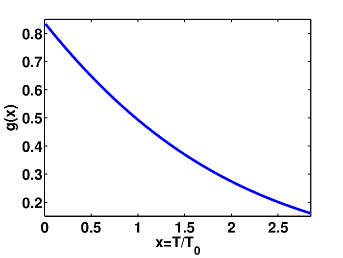
where erf is the error function and is its complement. The function characterizes the spectrum of the emitted electrons and is exhibited in Fig. 1 and it is without any particular structure, which is the case in most WIMP searches.
For a 50 keV sterile neutrino we find that:
Now . Thus
| (9) |
where
It is clear that with this amount of energy transferred to the electron it is not possible to eject an electron out of the atom. One therefore must use special materials such that the electrons are loosely bound. It has recently been suggested that it is possible to detect even very light WIMPS, much lighter than the electron, utilizing Fermi-degenerate materials like superconductors[57]. In this case the energy required is essentially the gap energy of about , which is in the meV region, i.e the electrons are essentially free. In what follows, we assume the values
| (10) |
while is taken as a parameter and will be discussed in section VII. Thus we obtain:
| (11) |
The neutrino particle density is
while the neutrino flux
where being the dark matter density. Assuming that the number of electron pairs in the target is we find that the number of events per year is
| (12) |
The authors of [57] are perhaps aware of the fact that the average energy for very light WIMPS is small and, as we have seen above, a small portion of it is transferred to their system . With their bolometer detector these authors probably have a way to circumvent the fact that a small amount of energy will be deposited, about 0.4 eV in a year for . Perhaps they may manage to accumulate a larger number of loosely bound electrons in their target.
III Sterile neutrino detection via low temperature bolometers
Another possibility is to use bolometers, like the CUORE detector exploiting Low Temperature Specific Heat of Crystalline 130TeO2 at low temperatures. The energy of the WIMP will now be deposited in the crystal, after its interaction with the nuclei via Z-exchange. In this case the Fermi component of interaction with neutrons is coherent, while that of the protons is negligible. Thus the matrix element becomes:
| (13) |
A detailed analysis of the frequencies the 130TeO2 can be found [58]. The analysis involved crystalline phases of tellurium dioxide: paratellurite -TeO2, tellurite -TeO2 and the new phase γ-TeO2, recently identified experimentally. Calculated Raman and IR spectra are in good agreement with available experimental data. The vibrational spectra of and -TeO2 can be interpreted in terms of vibrations of TeO2 molecular units. The -TeO2 modes are associated with the symmetry or 422, which has 5 irreducible representations, two 1-dimensional of the antisymmetric type indicated by and , two 1-dimensional of the symmetric type and and one 2-dimensional, usually indicated by . They all have been tabulated in Ref. [58]. Those that can be excited must be below the Debye frequency which has been determined [59] and found to be quite low:
This frequency is smaller than the maximum sterile neutrino energy estimated to be eV. Those frequency modes of interest to us are given in Table 1. The differential cross section is, therefore given by
| (14) |
where will be specified below and the momentum transferred to the nucleus. The momentum transfer is small and the form factor can be neglected.
In deriving this formula we tacitly assumed a coherent interaction between the WIMP and several nuclei, thus creating a collective excitation of the crystal, i.e. a phonon or few phonons. This of course is a good approximation provided that the energy transferred is small, of a few tens of meV. We see from table 1 that the maximum allowed energy is small, around 100 meV. We find that, if we restrict the maximum allowed energy by a factor of 2, the obtained results are reduced only by a factor of about . We may thus assume that this approximation is good.
Integrating over the nuclear momentum we get
| (15) |
| (16) |
performing the integration using the function we get
| (17) |
| (18) |
where
Folding
with the velocity distribution we obtain
| (19) | |||||
We see that we have the constraint imposed by the available energy, namely:
where integer part of . We thus find the listed in table 1. The functions are exhibited in fig. 2.


The relevant integrals are for , , for , , for and for . Thus we obtain a total of 17.8. The event rate takes with a target of mass takes the the form:
If we restrict the maximum allowed energy to half of that shown in
Table 1 by
a factor of two, we obtain 15.7 instead of 17.8.
For a 130TeO2 target (N=78) of 1 kg of mass get
This is much larger than that obtained in the previous section, mainly due to the neutron coherence arising from the Z-interaction with the target (the number of scattering centers is approximately the same . In the present case, however, targets can be larger than 1 kg. Next we are going to examine other mechanisms, which promise a better signature.
IV Sterile neutrino detection via atomic excitations
We are going to examine the interesting possibility of excitation of an atom from a level to a nearby level at energy , which has the same orbital structure. The excitation energy has to be quite low, i.e:
| (20) |
The target is selected so that the two levels and are closer han 0.11 eV. This can arise result from the splitting of an atomic level by the magnetic field so that they can be connected by the spin operator. The lower one is occupied by electrons but the higher one is completely empty at sufficiently low temperature. It can be populated only by exciting an electron to it from the lower one by the oncoming sterile neutrino. The presence of such an excitation is monitor by a tuned laser which excites such an electron from to a higher state , which cannot be reached in any other way, by observing its subsequent decay by emitting photons.
Since this is an one body transition the relevant matrix element takes the form:
| (21) |
(in the case of the axial current we have and we need evaluate the matrix element of and then square it and sum as well as average over the neutrino polarizations).
| (22) |
expressed in terms of the Glebsch-Gordan coefficient and the nine- j symbol. It is clear that in the energy transfer of interest only the axial current can contribute to excitation
The cross section takes the form:
| (23) |
Integrating over the atom recoil momentum, which has negligible effect on the energy, and over the direction of the final neutrino momentum and energy via the function we obtain
| (24) | |||||
| (25) |
where we have set .
Folding the cross section with the velocity distribution from a minimum to we obtain
| (26) |
Clearly the maximum excitation energy that can be reached is eV. The function is exhibited in Fig. 3

Proceeding as in section II and noting that for small excitation energy we find :
The expected rate will be smaller after the angular momentum factor is included (see appendix A). Anyway leaving aside this factor, which can only be determined after a specific set of levels is selected, we see that the obtained rate is comparable to that expected from electron recoil (see Eq. (12)). In fact for a target with we obtain:
This rate, however, decreases as the excitation energy increases (see Fig. 3). In the present case, however, we have two advantages.
- •
The characteristic signature of photons spectrum following the de-excitation of of the level mentioned above. The photon energy can be changed if the target is put in a magnetic field by a judicious choice of
- •
The target now can be much larger, since one can employ a solid at very low temperatures. The ions of the crystal still exhibit atomic structure. The electronic states probably won’t carry all the important quantum numbers as their corresponding neutral atoms. One may have to consider exotic atoms (see appendix B) or targets which contain appropriate impurity atoms in a host crystal, e.g Chromium in sapphire.
In spite of this it seems very hard to detect such a process, since the expected counting rate is very low.
V Sterile neutrino capture by a nucleus undergoing electron capture
This is essentially the process:
| (27) |
involving the absorption of a neutrino with the simultaneous capture of a bound electron. It has already been studied [60] in connection with the detection of the standard relic neutrinos. It involves modern technological innovations like the Penning Trap Mass Spectrometry (PT-MS) and the Micro-Calorimetry (MC). The former should provide an answer to the question of accurately measuring the nuclear binding energies and how strong the resonance enhancement is expected, whereas the latter should analyze the bolometric spectrum in the tail of the peak corresponding to L-capture to the excited state in order to observe the relic anti-neutrino events. They also examined the suitability of 157Tb for relic antineutrino detection via the resonant enhancement to be considered by the PT-MS and MC teams. In the present case the experimental constraints are expected to be less stringent since the sterile neutrino is much heavier.
Let us measure all energies from the ground state of the final nucleus and assume that is the mass difference of the two neutral atoms. Let us consider a transition to the final state with energy . The cross section for a neutrino11 1 Here as well as in the following we may write neutrino, but it is understood that we mean antineutrino of given velocity and kinetic energy is given by:
| (28) |
where is the recoiling nucleus momentum. Integrating over the recoil momentum using the function we obtain
| (29) |
We note that, since the oncoming neutrino has a mass, the excited state must be higher than the highest excited state at . Indicating by the above equation can be written as
| (30) |
Folding it with the velocity distribution as above we obtain:
| (31) |
or using the delta function
| (32) | |||||
| (33) |
As expected the cross section exhibits resonance behavior though the normalized function F(X) as shown in Fig. 4.

It is, of course, more practical to exhibit the function as a function of the the energy . This is exhibited in Fig.5. From this figure we see that the cross section resonance is quite narrow. We find that the maximum occurs at and has a width eV. So for all practical purposes it is a line centered at the neutrino mass. The width may be of some relevance in the special case whereby the excited state can be determined by atomic de-excitations at the sub eV level, but it will not show up in the nuclear de-excitations.

If there is a resonance in the final nucleus at the energy with a width then perhaps it can be reached even if is a bit larger than , e.g. . The population of this resonance can be determined by measuring the energy of the de-excitation -ray, which should exceed by the maximum observed in ordinary electron capture.
For antineutrinos having zero kinetic energy the atom in the final state has to have an excess energy and this can only happen if this energy can be radiated out via photon or phonon emission. The photon emission takes place either as atomic electron or nuclear level transitions. In the first case photon energies falling in the eV-keV energy region and this implies that only nuclei with a very small -value could be suitable for this detection. In the second case, there should exist a nuclear level that matches the energy difference and therefore the incoming antineutrino has no energy threshold. Moreover, spontaneous electron capture decay is energetically forbidden, since this is allowed for .
As an example we consider the capture of a very low energy by the Tb nucleus
| (34) |
taking the allowed transitions from the ground state () of parent nucleus, Tb, to the first excited state of the daughter nucleus Gd. The spin and parity of the nuclei involved obey the relations , , and the transition is dubbed as allowed. The nuclear matrix element can be written as can be written as
| (35) |
where and being the axial and vector coupling constants respectively. The nuclear matrix element is calculated using the microscopic quasi-particle-phonon (MQPM) model [61, 62] and it is found to be . The experimental value of first excited is at 64 keV [63] while the predicted by the model at 65 keV. The -value is ranging from 60 to 63 keV [63].
For K-shell electron capture where (1s capture) with binding energy keV, the velocity averaged cross section takes the value
and the event rate we expect for mass kg is
| (36) |
The life time of the source should be suitable for the experiment to be performed. If it is too short, the time available will not be adequate for the execution of the experiment. If it is too long, the number of counts during the data taking will be too small. Then one will face formidable backgrounds and/or large experimental uncertainties.
The source should be cheaply available in large quantities. Clearly a compromise has to be made in the selection of the source. One can be optimistic that adequate such quantities can be produced in Russian reactors. The nuclide parameters relevant to our work can be found in [64] (see also [65]), summarized in table 2.
| Nuclide | EC transition | (keV) | (keV) | (keV) | (keV) | |
|---|---|---|---|---|---|---|
| 157Tb | 71 y | 3/2 | 60.04(30) | K: 50.2391(5) | LI: 8.3756(5) | 9.76 |
| 163Ho | 4570 y | 7/2 | 2.555(16) | MI: 2.0468(5) | NI: 0.4163(5) | 0.51 |
| 179Ta | 1.82 y | 7/2 | 105.6(4) | K: 65.3508(6) | LI: 11.2707(4) | 40.2 |
| 193Pt | 50 y | 1/2 | 56.63(30) | LI: 13.4185(3) | MI: 3.1737(17) | 43.2 |
| 202Pb | 52 ky | 0 | 46(14) | LI: 15.3467(4) | MI: 3.7041(4) | 30.7 |
| 205Pb | 13 My | 5/2 | 50.6(5) | LI: 15.3467(4) | MI: 3.7041(4) | 35.3 |
| 235Np | 396 d | 5/2 | 124.2(9) | K: 115.6061(16) | LI: 21.7574(3) | 8.6 |
VI Modification of the end point spectra of decaying nuclei
The end point spectra of decaying nuclei can be modified by the reaction involving sterile (anti)neutrinos
| (37) |
or
| (38) |
This can be exploited in on ongoing experiments, e.g. in the Tritium decay
| (39) |
The relevant cross section is:
| (40) |
where is the atomic mass difference. Integrating over the nuclear recoil momentum and the direction of the electron momentum we get:
| (41) |
where
| (42) |
and
| (43) |

Folding the cross section with the velocity distribution we find
| (44) |
where
| (45) |
with
The Fermi function, encapsulates the effects of the Coulomb interaction for a given lepton energy and final state proton number . The function is exhibited in Fig. 6.
In transitions happening inside the same isospin multiplet () both the vector and axial form factors contribute and in this case the nuclear matrix element can be written as can be written as
| (46) |
where and being the axial and vector coupling constants respectively. In case of target we adopt and from [67]. Thus .
Thus the velocity averaged cross section takes the value
and the expected event rate becomes
| (47) |
For a mass of the current KATRIN target, i.e. about 1 gr, we get
| (48) |
It is interesting to compare the neutrino capture rate
| (49) |
with that of beta decay process , whose rate is given by
| (50) |
where is the maximal electron energy or else beta decay endpoint
| (51) |
with
| (52) |
the electron kinetic energy at the endpoint, and
| (53) | |||
| (54) | |||
| (55) |
Masses and are nuclear masses [66, 68, 56]. The calculation of (50) gives . The ratio of to corresponding beta decay is very small.
| (56) |
The situation is more optimistic in a narrow interval near the endpoint. As an example, we consider an energy resolution eV close to the expected sensitivity of the KATRIN experiment [55]. Then the ratio of the event rate to that of neutrino capture gives

In fig. 7 we present the ratio of the event rate decay rate of for the beta decay compared with the neutrino capture rate as a function of the energy resolution in the energy region
Moreover, the electron kinetic energy due to neutrino capture process (39) is
| (57) |
this means that the electron in the final state has a kinetic energy of at least above the corresponding beta decay endpoint energy. There is no reaction induced background there, but, unfortunately, the ratio obtained above is much lower than the expected KATRIN sensitivity.
VII Discussion
In the present paper we examined the possibility of direct detection of sterile neutrinos of a mass 50 keV, in dark matter searches. This depends on finding solutions to two problems. The first is the amount of energy expected to be deposited in the detector and the second one is the expected event rate. In connection with the energy we have seen that, even though these neutrinos are quite heavy, their detection is not easy, since like all dark matters candidates move in our galaxies with not relativistic velocities, c on the average and with energies about 0.05 eV, not all of which can be deposited in the detectors. Thus the detection techniques employed in the standard dark matter experiments, like those looking for heavy WIMP candidates, are not applicable in this case.
We started our investigation by considering neutrino electron scattering. Since the energy of the sterile neutrino is very small one may have to consider systems with very small electron binding, e.g. electron pairs in superconductors, which are limited to rather small number of electron pairs. Alternatively one may use low temperature bolometers, which can be larger in size resulting in a higher expected event rate. These experiments must be able to detect very small amount of energy.
Then we examined more exotic options by exploiting atomic and nuclear physics. In atomic physics we examined the possibility of spin induced excitations. Again to avoid background problems the detector has to a crystal operating at low temperatures. Then what matters is the atomic structure of the ions of the crystal or of suitably implanted impurities. The rate in this case is less than that obtained in the case of bolometers, but one may be able to exploit the characteristic feature of the spectrum of the emitted photons.
From the nuclear physics point of view, we consider the antineutrino absorption on an electron capturing nuclear system leading to a fine resonance in the (N+1,Z-1) system, centered 50 keV above the highest excited state reached by the ordinary electron capture. The de-excitation of this resonance will lead to a very characteristic ray. Finally the sterile neutrino will lead to A(N,Z)+A(N-1,Z+1) reaction. The produced electrons will have a maximum energy which goes beyond the end point energy of the corresponding decay by essentially the neutrino mass. The signature is less profound than in the case of antineutrino absorption.
Regarding the event rate, as we have mentioned before, it is proportional to the coupling of the sterile neutrino to the usual electron neutrino indicated above as . This parameter is not known. In neutrino oscillation experiments a value of has been employed. With such a value our results show that the 50 keV neutrino is detectable in the experiments discussed above. This large value of is not consistent, however, with a sterile 50 kev neutrino. In fact such a neutrino would have a life time [69] of y, much shorter than the age of the universe. A cosmologically viable sterile 50 keV neutrino is allowed to couple to the electron neutrino with coupling . Our calculations indicate that such a neutrino is not directly detectable with experiments considered in this work. The results, however, obtained for the various physical processes considered in this work, can be very useful in the analysis of the possible experimental searches of lighter sterile neutrinos in the mass range of 1-10 keV.
Acknowledgements: The authors are indebted to professor Marco Bernasconi for useful suggestions in connection with the phonon excitations of low temperature bolometers.
References
- [1] P. Ullio and M. Kamioknowski, JHEP 0103, 049 (2001).
- [2] D. Spergel et al., Astrophys. J. Suppl. 170, 377 (2007), [arXiv:astro-ph/0603449v2].
- [3] P. A. R. Ade et al., Astronomy and Astrophysics 571, A31 (2014), the Planck Collaboration, arXiv:1508.03375 (astro-ph.CO).
- [4] A. Bottino et al., Phys. Lett B 402, 113 (1997).
- [5] R. Arnowitt and P. Nath, Phys. Rev. Lett. 74, 4592 (1995).
- [6] R. Arnowitt and P. Nath, Phys. Rev. D 54, 2374 (1996), hep-ph/9902237.
- [7] V. A. Bednyakov, H. Klapdor-Kleingrothaus, and S. Kovalenko, Phys. Lett. B 329, 5 (1994).
- [8] J. Ellis and L. Roszkowski, Phys. Lett. B 283, 252 (1992).
- [9] J. Ellis, and R. A. Flores, Phys. Lett. B 263, 259 (1991); Phys. Lett. B 300, 175 (1993); Nucl. Phys. B 400, 25 (1993).
- [10] S. Nussinov, Phys. Lett. B 279, 111 (1992).
- [11] S. B. Gudnason, C. Kouvaris, and F. Sannino, Phys. Rev. D 74, 095008 (2006), arXiv:hep-ph/0608055.
- [12] R. Foot, H. Lew, and R. R. Volkas, Phys. Lett. B 272, 676 (1991).
- [13] R. Foot, Phys. Lett. B 703, 7 (2011), [arXiv:1106.2688].
- [14] G. Servant and T. M. P. Tait, Nuc. Phys. B 650, 391 (2003).
- [15] V. Oikonomou, J. Vergados, and C. C. Moustakidis, Nuc. Phys. B 773, 19 (2007).
- [16] M. W. Goodman and E. Witten, Phys. Rev. D 31, 3059 (1985).
- [17] J. Angle et al, arXiv:1104.3088 [hep-ph].
- [18] E. Aprile et al., Phys. Rev. Lett. 107, 131302 (2011), arXiv:1104.2549v3 [astro-ph.CO].
- [19] K. Abe et al., Astropart. Phys. 31, 290 (2009), arXiv:v3 [physics.ins-det]0809.4413v3 [physics.ins-det].
- [20] C. Ghag et al., Astropar. Phys. 35, 76 (2011), arXiv:1103.0393 [astro-ph.CO].
- [21] See, e.g., Kaixuan Ni, Proceedings of the Dark Side of the Universe, DSU2011, Beijing, 9/27/2011.
- [22] D.C. Malling it et al, arXiv:1110.0103((astro-ph.IM)).
- [23] D. Akerib et al., Phys. Rev. Lett. 96, 011302 (2006), arXiv:astro-ph/0509259 and arXiv:astro-ph/0509269.
- [24] C. Aalseth et al., Phys. Rev. Lett. 106, 131301 (2011), coGeNT collaboration arXiv:10002.4703 [astro-ph.CO].
- [25] E. Armengaud et al., Phys. Lett. B 702, 329 (2011), arXiv:1103.4070v3 [astro-ph.CO].
- [26] R. Bernabei and Others, Eur. Phys. J. C 56, 333 (2008), [DAMA Collaboration]; [arXiv:0804.2741 [astro-ph]].
- [27] P. Belli et al, arXiv:1106.4667 [astro-ph.GA].
- [28] H. S. Lee et al., Phys.Rev.Lett. 99, 091301 (2007), arXiv:0704.0423[astro-ph].
- [29] S. Archambault et al., Phys. Lett. B 682, 185 (2009), the PICASSO collaboration, arXiv:0907.0307 [astro-ex].
- [30] S. Archambault et al., New J. Phys. 13, 043006 (2011), arXiv:1011.4553 (physics.ins-det).
- [31] C. R. Arguelles, N. E. Mavromatos, J. A. Rueda, and R. Ruffini, JCAP 1604, 038 (2016), arXiv:1502.00136.
- [32] R. Ruffini, C. R. Arguelles, and J. A. Rueda, MNRAS 451, 622 (2016).
- [33] C. R Arguelles and R. Ruffini and J. A. Rueda, arXiv:1606.07040.
- [34] A. Boyarsky, O. Ruchayskiy, and M. Shaposhnikov, Review of Nuclear and Particle Science 59, 191 (2009a).
- [35] A. Boyarsky, J. Lesgourgues, O. Ruchayskiy, and M. Viel, PRL 102, 201304 (2009b).
- [36] E. J. Tollerud, J. S. Bullock, L. E. Strigari, and B. Willman, ApJ 688, 277 (2008).
- [37] M. D. Campos and W. Rodejohann, Phys. Rev. D 94, 095010 (2016).
- [38] Y. Li and Z. zhong Xing, Phys. Lett. B 695, 205 (2011a).
- [39] Y. Li and Z. zhong Xing, JCAP 1108, 006 (2011b).
- [40] Giorgio Arcadia et al., arXiv:1703.07364v1.
- [41] W. Liao, Phys. Rev. D 82, 073001 (2010).
- [42] R. Adhikari al , A White Paper on keV Sterile Neutrino Dark Matter, arXiv:1602.04816 [hep-ph].
- [43] A. Aguilar-Arevalo et al., Phys. Rev D 64, 112007 (2001), lSND Collaboration.
- [44] A. Aguilar-Arevalo et al., Phys. Rev Lett. 110, 161801 (2013), miniBooNE Collaboration.
- [45] T. Katori and J. M. Conrad, Adv. High Energy Phys. 2015, 362971 (2015), miniBooNE Collaboration.
- [46] T. A. Mueller et al., Phys. Rev. C 83, 054615 (2011).
- [47] J. N. Abdurashitov et al., Phys. Rev. C 73, 045805 (2006).
- [48] J. Kopp, P. A. N. Machado, M. Maltoni, and T. Schwetz, J. High Energy Phys. 1305, 050 (2013).
- [49] C. Giunti, M. Laveder, Y. F. Li, and H. W. Long, Phys. Rev. D 88, 073008 (2013).
- [50] G. Mention et al., Phys. Rev. D 83, 073006 (2011).
- [51] T. Asaka and S. B. M. Shaposhnikov, Phys. Lett. B 631, 151 (2005), [hep-ph/0503065].
- [52] S. Kusenko, Phys. Rep. 481, 1 (2009), [arXiv:0906.2968].
- [53] L. Heurtier and D. Teresi, Phys. Rev. D 94, 125022 (2016), [arXiv:1607.01798].
- [54] N. M. Mvromatos and A. Pilaftsis, Phys. Rev. D 86, 124028 (2012), arXiv:1209.6387.
- [55] A. Osipowitcz et al,[KATRIN Collaboration], 2001 arxiv:hep-ex/0109033.
- [56] J. Beringer et al., Phys. Rev. D 86, 010001 (2012).
- [57] Y. Hocberg,M. Pyle, Y. Zhao and M, Zurek, Detecting superlight Dark Matter with Fermi Degenerate Materials, arXiv:1512,04533 [hep-ph].
- [58] M. Ceriotti, F. Pietrucci, and M. Bernasconi, Physical Review B 73, 104304 (2006), arXiv:0803.4056 [cond-mat.mtrl-sci].
- [59] M. Barucci, C. Brofferio, A. Giuliani, E. Gottardi, I. Peroni, and G. Ventura, Journal of Low Temperature Physics 123(5), 303 (2001).
- [60] J. Vergados and Y. N. Novikov, J. Phys. G: Nucl. and Part. Phys. 41, 125001 (2014), arXiv:1312.0879 [hep-ph].
- [61] J. Toivanen and J. Suhonen, J. Phys. G 21, 1491 (1995).
- [62] J. Toivanen and J. Suhonen, Phys. Rev. C 57, 1237 (1998).
- [63] R. G. Helmer, Nucl. Data Sheets 103, 565 (2004).
- [64] P. E. Filianin, K. Blaum, S. A. Eliseev, L. Gastaldo, Y. N. Novikov, V. M. Shabaev, I. I. Tupitsyn, and J. D. Vergados, J. Phys. G, Nuc. Par. Phys. 41 (9), 095004 (2014), [arXiv:1402.4400].
- [65] J. Vergados and Y. N. Novikov, Nuc. Phys.B 831, 1 (2010), arXiv:1006.3862 [pdf, ps, other] [hep-ph].
- [66] G. Audi, A. Wapstra, and C. Thibault, Nuc. Phys. A 729, 337 (2002).
- [67] R. Schiavilla et al., Phys. Rev C 58, 1263 (i998), [arXiv:nucl-th/9808010].
- [68] J. A. Bearden and A. F. Burr, Rev. Mod. Phys 39, 125 (1967).
- [69] A.Dolgov and S.Hansen, Astropart. Phys. 16, 339 (2002), [hep-ph/0009083].
- [70] M. W. Doherty, N. B. Manson, P. Delaney, F. Jelezko, J. Wrachtrup, and L. C. L. Hollenberg, Phys. Rep. 528, 1 (2013), arXiv:1302.3288.
VIII Appendix A: Angular momentum coefficients entering atomic excitations.
IX Appendix B: Exotic atomic experiments
As we have mentioned the atomic experiment has to be done at low temperatures. It may be difficult to find materials exhibiting atomic structure at low temperatures, It amusing to note that one may be able to employ at low temperatures some exotic materials used in quantum technologies (for a recent review see [70]) like nitrogen-vacancy (NV), i.e. materials characterized by spin , which in a magnetic field allow transitions between and . These states are spin symmetric. Antisymmetry requires the space part to be antisymmetric, i.e. a wave function of the form
Of special interest are:
Then the spin matrix element takes the form:
The reduced matrix elements are given in table 5, as well as the full matrix element of the most important component.