The clustering of galaxies: Predictions from the BLUETIDES simulation
Abstract
We study the clustering of the highest- galaxies (from to a few tens Mpc scales) using the BLUETIDES simulation and compare it to current observational constraints from Hubble legacy and Hyper Suprime Cam (HSC) fields (at ). With a box length of 400 Mpc/ on each side and 0.7 trillion particles, BLUETIDES is the largest volume high resolution cosmological hydrodynamic simulation to date ideally suited for studies of high galaxies. We find that galaxies with magnitude have a bias () of at , and typical halo masses . Given the redshift evolution between to (), our inferred values of the bias and halo masses are consistent with measured angular clustering at from these brighter samples. The bias of fainter galaxies (in the Hubble legacy field at ) is at corresponding to halo masses . We investigate directly the 1-halo term in the clustering and show that it dominates on scales Mpc/ () with non-linear effect at transition scales between the 1-halo and 2-halo term affecting scales 0.1 20 Mpc/ (). Current clustering measurements probe down to the scales in the transition between 1-halo to 2-halo regime where non-linear effects are important. The amplitude of the 1-halo term implies that occupation numbers for satellites in BLUETIDES are somewhat higher than standard HODs adopted in these analyses (which predict amplitudes in the 1-halo regime suppressed by a factor 2-3). That possibly implies a higher number of galaxies detected by JWST (at small scales and even fainter magnitudes) observing these fields.
Keywords:
galaxies: high-redshift – galaxies: evolution – galaxies: formation – galaxies: haloes – galaxies: statistics – cosmology: theory – large-scale structure of Universe1 Introduction
Advancement of observational techniques and the emergence of more powerful telescopes have pushed the observational frontiers to increasingly higher redshifts. Detecting the earliest galaxies holds the key to understanding the role of the first galaxies in triggering the epoch of reionization. The study of Lyman Break Galaxies (LBGs) is one such probe with a number of candidate objects detected by the HST fields to redshifts as far as (Oesch et al., 2016; Bouwens et al., 2016; McLeod et al., 2016). Upcoming satellites such as the James Web Space Telescope (JWST) and the Wide Field Infrared Survey Telescope (WFIRST-AFTA) are expected to detect a large number of objects at redshifts 8-15 (Waters et al., 2016b).
Performing clustering analysis for these distant galaxies () poses a major challenge due to 1) not having enough objects to obtain reliable statistics 2) presence of cosmic variance for narrow fields of survey (Trenti & Stiavelli, 2008; Robertson et al., 2014; Somerville et al., 2004). For instance, HST WFC 3 has a 2 arcmin IR field of view, and is therefore subjected to substantial amount of cosmic variance. JWST will observe at greater depths and hence detect more objects, but will likely have a similar degree of cosmic variance. WFIRST will have a survey area of which is comparable to that of ground based survey, and will have a depth comparable to that of HST-Ultra Deep Field. Spergel et al. (2013) predicts a limiting magnitude of and respectively for the WFIRST. WFIRST observations will be amongst the first to reliably capture the clustering of the brightest galaxies at , some of the predictions of which have been made by Waters et al. (2016b).
Despite the foregoing difficulties, clustering studies have been performed for medium to high galaxies within the later half of the reionization epoch and after. Ishikawa et al. (2015) analyzed the clustering properties at using the data taken at the United Kingdom Infrared telescope and Canada-France-Hawaii Telescope (CFHT). Hildebrandt et al. (2009) obtained the angular correlation functions of Lyman Break Galaxies (LBGs) at using the observations of Canada-France-Hawaii Telescope Legacy Survey (CFHTLS). Ouchi et al. (2001) performed clustering studies at using the data taken at the Subaru deep survey. Munshi et al. (2004) took a compilation of a number of surveys and studied the evolution of galaxy clustering from to . Similarly, Adelberger et al. (2005) compiled star forming galaxies from multiple surveys and studied their spatial clustering at redshifts . Owing to the data collected by the Hubble Space Telescope Wide field camera 3 (HST-WFC3), the observation frontier for large scale clustering has been pushed to . Barone-Nugent et al. (2014) estimated the angular clustering of LBG galaxies at redshifts upto using a combined sample of LBGs from HST-WFC3, Hubble eXtreme Deep Field (XDF) and CANDELS surveys; and thereafter for the first time estimates the large scale linear bias at by fitting the angular correlation function to a power-law model. Harikane et al. (2016) and Harikane et al. (2017) further expanded the compilation by including the Hubble Frontier Field (HFF) and the HSC SSP(Subaru) data and made improved estimates of the angular clustering and the large scale bias.
The clustering measurements of observed galaxy samples enable us to simultaneously constrain cosmology, as well as physics of galaxy formation; this is typically done using Halo Occupation Distribution (HOD) modelling (Berlind & Weinberg, 2002). Incorporating the HODs into the framework of the halo model (Cooray & Sheth, 2002), one can study galaxy clustering and fit model parameters to observational measurements, thereby determining the average halo masses and biases of the observed galaxy subsamples i.e. the galaxy-dark matter halo connection. This has been extensively applied to low () to medium () redshift measurements (Zehavi et al., 2005; Zheng et al., 2007; van den Bosch et al., 2013; Bullock et al., 2002; Hamana et al., 2004; Bian et al., 2013; Hildebrandt et al., 2007)). Recent studies have started focusing on the application of HOD modelling to galaxies within the reionization epoch (Harikane et al., 2016; Harikane et al., 2017; Hatfield et al., 2017).
Semi-analytical (SA) models (Benson, 2012; Cousin et al., 2015; Cattaneo et al., 2017; Hou et al., 2017, and references therein) have also been extensively used to predict the clustering as well as other intrinsic properties of galaxies. Several studies using SA models have been performed to predict galaxy clustering at high redshifts. Baugh et al. (1998) constructs mock galaxy catalogs and reports broad agreement with observations existing at that time. Park et al. (2016) studies clustering of LBGs at using semi analytical models and finds good agreement with the measurements of Hubble eXtreme Depp Field (XDF) and CANDELS fields. Kashikawa et al. (2006) also analyzes clustering of LBG galaxies from the Subaru deep field at and achieves good agreement with the results obtained from a mock galaxy catalog constructed using semi-analytical modelling. Jose et al. (2013) builds SA models to predict clustering of high redshift galaxies and achieves excellent agreement with observations from . Jose et al. (2016), Jose et al. (2017) use N-body simulations to study clustering of dark matter halos at high redshifts () and reveal the existence of non-linear bias in the two-halo regime at these redshifts. More recently, Park et al. (2017) used N-body + semianalytic models to make predictions of clustering of LBGs upto , and shows that they agree well with current measurements upto . As we shall show later, their predictions at agree well with BLUETIDES.
Recently there has been tremendous progress in cosmological hydrodynamic simulations of galaxy formation. Capturing (as much of) the relevant physics at small scales while simulating statistical populations of galaxies demands a combination of having a large volume, as well as having large enough number of resolution elements. Several large scale simulations have been performed in the recent years in order to study the formation of the first galaxies and their roles in the epoch of reionization. MASSIVE BLACK I (Di Matteo et al., 2012) has a box length of and was run to . Its successor, MASSIVE BLACK II had a smaller box length of and therefore had a higher resolution (Khandai et al., 2015); it was run to . MASSIVE BLACK II illustrated that the inclusion of baryons have strong effects on the abundances of dark matter halos, which motivated more simulations of such kind. ILLUSTRIS (Nelson et al., 2015) was similar to MASSIVE BLACK II in terms of simulation volume as well as resolution, but with improved modelling for SN II feedback (Okamoto et al., 2010). EAGLE simulation (Schaye et al., 2015) is also comparable to that of ILLUSTRIS and MASSIVE BLACK II, but with improved modelling of sub-grid physics which lead to better agreement with observations.
In order to study clustering at high redshifts, large volume simulations are required (the high-z galaxy populations are rare-bright objects). Here we use the BLUETIDES simulation (Feng et al., 2016) with a box side qlength of 400 Mpc/ and has a particle load 10 times that of MASSIVE BLACK I. Due to high particle load, the resolution is comparable to that of MASSIVE BLACK II or ILLUSTRIS, which makes it the largest high resolution cosmological simulation performed to date. The flipside to this is that the simulation is so computationally demanding that it has currently been run only down to . While attempts are being made to push the simulation further down to lower redshifts here we wish to first further validate BLUETIDES by examining the predictions for galaxy clustering and compare to current constraints. The photometric properties of the BLUETIDES galaxies have been calculated in Wilkins et al. (2016) using five different stellar population synthesis models. The predicted luminosity functions and star formation rates show good consistency with the currently available observations at (Feng et al., 2016); the resolution is high enough to obtain the slope of the faint end of the luminosity function which is consistent with Bouwens et al. (2014). BLUETIDES also consistently predicted the properties of GN-z11 (Oesch et al., 2016) which is the farthest galaxy observed to date (Waters et al., 2016a). BLUETIDES forecasts for the upcoming WFIRST satellite have been made by Waters et al. (2016b) and results look promising with about predicted galaxies from upto . In the large volume of BLUETIDES it has also been possible to study the formation of the first quasars, supermassive black holes (Di Matteo et al., 2017).
In this work, we perform a detailed analysis of the clustering of BLUETIDES galaxies at redshifts . We predict clustering properties of observed galaxy samples at (Bouwens et al., 2015, hereafter B15), and estimate their typical biases and threshold halo masses. We investigate the redshift evolution of the clustering and compare to current clustering measurements at lower redshifts (Harikane et al., 2016, hereafter H16). We compare our clustering results, particularly the one-halo term, to the predictions of an HOD model, and highlight some differences between them at various length scales.
2 The Bluetides simulation
| Description | Parameter | Value |
|---|---|---|
| Dark energy density | 0.7186 | |
| Matter density(Dark matter+Baryons) | 0.2814 | |
| Baryon density | 0.0464 | |
| Dimensionless Hubble parameter | h | 0.697 |
| Linear mass dispersion at | 0.82 | |
| Mass of dark matter particle | ||
| Mass of a gas particle | ||
| Seed mass of Black hole | ||
| Gravitational soothening length |
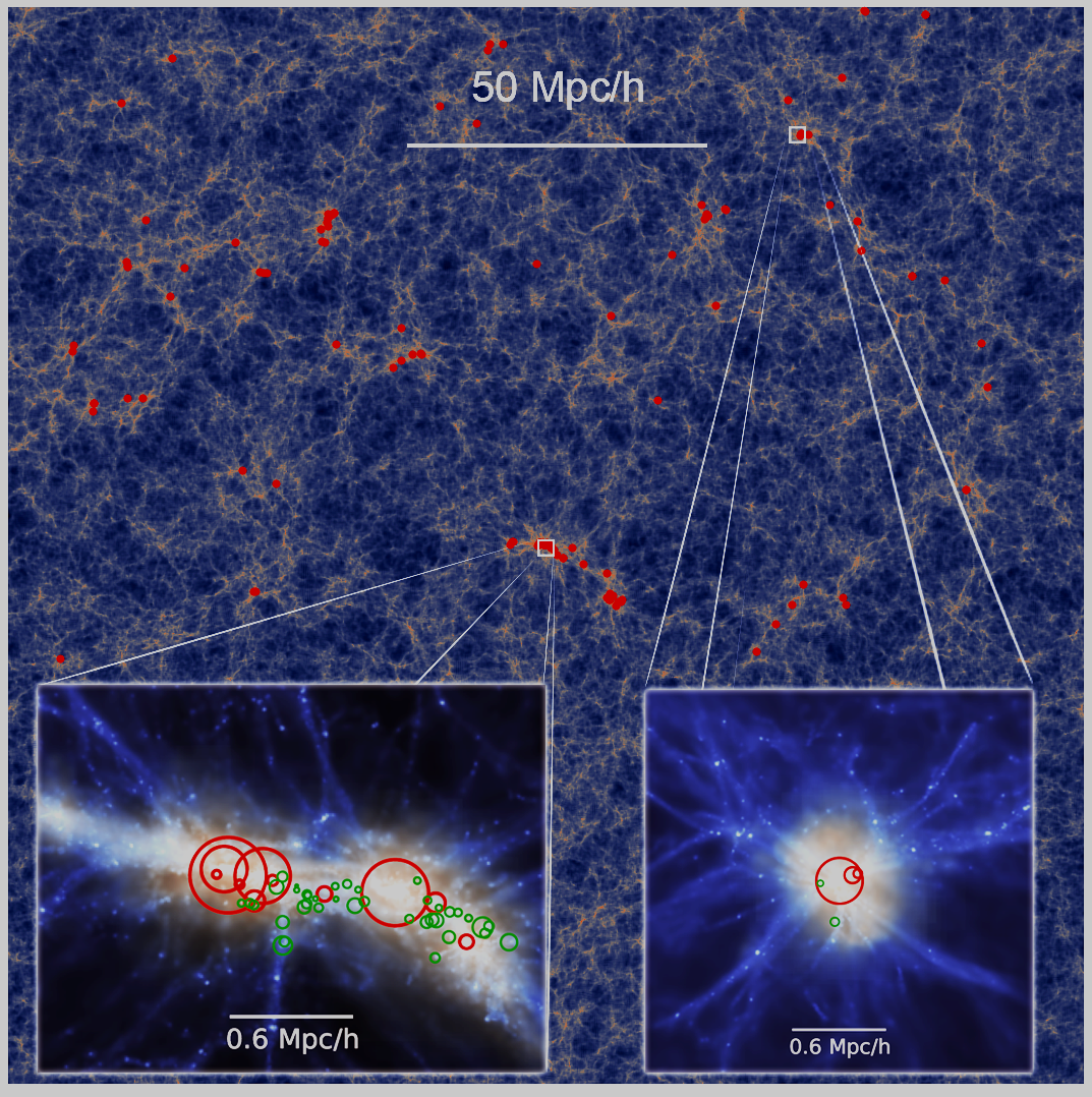
BLUETIDES was run on the Bluewaters super-computer at the National center for Computing applications. It essentially required the entire infrastructure of Bluewaters which comprises of 20250 nodes (648000 core equivalents). BLUETIDES is built upon on the precursor code MP-GADGET, to which substantial improvements were made to the parallel infrastructure in order to run at Petascale and exploit the full computing power of Bluewaters. Table 1 summarizes the important parameters used in BLUETIDES; a full discussion on the specific features is published in Feng et al. (2016). The Bluetides simulation employs the pressure-entropy formulation of Smooth Particle Hydrodynamics. The simulation is performed inside a comoving rectangular volume having a length of on each side. The total number of particles is about 0.7 trillion. The ensuing high resolution enables us to perform an extensive study of the formation of the first galaxies which may have driven reionisation, via detailed modelling of sub-grid physics described in 2.1. In addition to the high resolution, the extraordinarily high volume further allows us to study the large scale clustering of galaxies and dark matter halos. Overdensities were mapped using the Friend-of-Friends (FOF) groups identifier (Davis et al., 1985) with a linking length of 0.2 times the average spacing between the particles. The first FOF groups are identified at and their evolution is traced to . The simulation is about 300 times larger than the largest observational survey at (Trenti et al., 2010; Trenti et al., 2011). The substructure within the primary FOF groups were identified using ROCKSTAR-GALAXIES (Behroozi et al., 2013). While there are ongoing efforts to push the simulation further down to low redshifts (), the focus of our present work is on galaxies at redshifts 8,9 and 10. A visualization of the large-scale structure at is shown in Figure 1. The base panel is a slice of thickness 2 Mpc/, which shows the positions of the subhalos hosting galaxies with within the large scale density profile of dark matter. We also zoom in to reveal the gas temperature profiles of the substructures (shown as insets) of two FOFgroups of masses (left) and (right). The red circles show the positions and virial radii of galaxies with . As we shall see later, this threshold absolute magnitude corresponds to one of the observed samples obtained from HSC and Hubble legacy fields at , and in the following sections we are going to present a detailed clustering analysis of the entire sample of these galaxies residing within the BLUETIDES volume. We have also shown in green circles, an additional set of subhalos hosting fainter galaxies which are expected to be observed by the future deep field surveys of JWST. The galaxies in these FOFGroups have stellar masses ranging from to and star formation rates ranging from to .
In order to calculate the UV_luminosities, we use the PEGASE-v2 (Fioc & Rocca-Volmerange, 1997) stellar population synthesis (SPS) model along with the Chabrier (2003) initial mass function. The cumulative spectral energy distributions (SEDs) for each galaxy is calculated from SEDs for each star particle (as a function of stellar age and metallicity). The choice of the SPS model or the initial mass function makes a difference of at most 0.2 dex in the predicted luminosities (Wilkins et al., 2016), which is not large enough to significantly impact our final results. For a complete discussion of the photometric properties of BLUETIDES we urge the readers to refer to Wilkins et al. (2016).
2.1 Sub grid physics modelling
A number of sub grid physics models were invoked in order to study their influence on galaxy properties. To incorporate star formation, a multi star formation model as prescribed in Springel & Hernquist (2003) has been implemented. Gas cooling through radiative transfer and metal cooling are implemented using models of Katz et al. (1996) and Vogelsberger et al. (2014) respectively. We account for the effects of molecular hydrogen in the estimation of the star formation rate at low metallicities. Formation of molecular hydrogen is modelled by the prescription of Krumholz & Gnedin (2011). The modelling of type II Supernovae (SNII) feedback is performed according to Okamoto et al. (2010). The modelling of Active Galactic Nuclei (AGN) is the same as that performed in the MASSIVE BLACK I and II simulations (Di Matteo et al., 2012; Khandai et al., 2015). Black holes of masses are seeded at the local potential minima of halos with masses exceeding . The resulting feedback energy is deposited within a spherical volume of radius twice that of the SPH smoothing kernel of the black hole. The large volume of the simulation also enables us to estimate the effects of ”patchy” reionization, wherein the semianalytical modelling is applied to identify spatial regions which would be ionized at a given redshift; for further details we urge the readers to refer Feng et al. (2016) and Battaglia et al. (2013).
2.2 Clustering
The large volume and high resolution of the simulation enables us to study clustering of galaxies and dark matter halos at large scales as well as small scales. The clustering may be quantified by the spatial correlation function (in configuration space), or the 3D power spectrum (in Fourier space). The spatial correlation measures an excess in the pair-wise distribution of particles compared to the random uniform distribution and may be defined as
| (1) |
where is the total number of particles at a distance paired with a particle sitting at the origin, is the volume density for a uniform distribution and is the volume of the spherical shell at radius . For the bluetides data, we compute the galaxy and dark matter correlation functions ( and via brute force massively parallel pair counting using the KDCOUNT package (https://github.com/rainwoodman/kdcount).
The linear and non-linear regimes can be identified by computing the scale-dependent galaxy bias defined as,
| (2) |
At large scales we expect the bias to be constant (Mo & White, 1996; Sheth & Tormen, 1999; Tinker et al., 2010) whereas at small scales there is an onset of scale dependence in the bias due to non-linear effects (Jose et al., 2016). We also expect a steep increase in the bias as we go down to scales smaller than the typical halo radii due to a rise in the one halo contribution.
The angular correlation function can be obtained by projecting using the Limber projection formula,
| (3) |
where , is the comoving distance and is the normalized redshift distribution.
3 Halo Occupation Distribution (HOD) modelling
The main results in this work are based on analysing the clustering of high-z galaxies in the BLUETIDES simulation. We will however also attempt to reproduce the HOD models used by H16 as well. This allows us to compare directly simulations and HODs for these high-z galaxies.
For completeness, here we review briefly the standard assumptions used when building HODs and in particular those used in H16. HOD modelling is a commonly used technique to obtain the galaxy halo connection from clustering measurements. The key assumption is that the HOD i.e. the probability distribution of the number of galaxies for a given halo of mass , is dependent only on the halo mass. The occupation is therefore given by
| (4) |
where and are the mean number of central and satellite galaxies respectively. The mean occupations of central and satellite galaxies are given by,
| (5) |
| (6) |
is effectively a smoothened step function with being the width of transition between 0 to 1. The non-zero width of the transition is supposed to quantify the scatter in the Halo mass-luminosity relation. is the mass of the host halo at which 50 percent of the host halos contain a central galaxy. is assumed to be power law for halos above a cutoff mass of ; is the power law exponent and is referred as the slope of the power law.
Assuming that both and are independent of each other and is a Poisson distribution, the first moment of is given by
| (7) |
One can similarly obtain higher order moments but in the current context, we focus on the two point correlation function which is completely determined by the zeroth and first order moments of the HOD.
The mean density of galaxies at redshift is given by
| (8) |
where is the halo mass function. The factor DC is referred to as the Star formation duty cycle, defined as the probability of observing an existing star forming galaxy. DC is often less than unity because of the episodic nature of star formation activity (Stark et al., 2009). While DC is an important parameter in an HOD model, it does not affect galaxy clustering as along as it is independent of Halo mass. Thus, in our work we assume DC=1 as is done in Harikane et al. (2017).
The power spectrum is written as
| (9) |
where 1h and 2h represents the one-halo and two-halo contributions respectively. The one-halo term is further divided into central-satellite (cs) and satellite-satellite (ss) components,
| (10) |
| (11) |
| (12) |
The two-halo term is given by
| (13) |
where is the dark matter power spectrum, is the large scale/linear bias of halos of mass , is the mass function, is the fourier transform of the satellite galaxy density profile normalized by the halo mass. We keep our considerations identical to that of H16. We use the mass function from Behroozi et al. (2013) which essentially applies a correction factor to Tinker et al. (2008) for high redshifts, is obtained from Tinker et al. (2010). presumably traces the darkmatter distribution which is assumed to be NFW (Navarro et al., 1996) with a mass-concentration relation taken from Shimizu et al. (2003).
The angular correlation function can be obtained from using the Limber projection for the power spectrum,
| (14) |
where is the order Bessel function of the first kind, is the normalized redshift distribution and is the comoving distance as a function of redshift.
4 Results
In this section, we show some of the main properties of the galaxies in BLUETIDES as a function of their halo mass. We then move to the results on the clustering and compare to current observational measurements.
4.1 Galaxy-Halo connection in BLUETIDES

Figure 2 shows three relationships between the the halo mass , UV absolute magnitude (), Star formation rate (SFR) and stellar to halo mass ratio (SHMR) for the full galaxy population in BLUETIDES. The 2D histograms show the galaxies at while the solid lines are the mean relations at (blue, red and green respectively). The observational data points are from H16 at . The halo masses in the observed data are inferred using HOD modelling of the clustering. The BLUETIDES simulation clearly reproduced the overall properties of the observed galaxies. From the vs relation, we see that at fixed the host halos have higher masses at lower redshifts. vs SHMR also indicates larger halo mass for a fixed SHMR with decreasing redshifts. This indicates that at these redshifts, the halo mass assembly proceeds more efficiently than stellar mass. The foregoing trends are in broad agreement with the H16 observations for at , (which continues to be so till but for , H16 measurements show a reversal in this trend). Updated measurements in Harikane et al. (2017) at show the same trends; however no evidence of evolution was found in . This is also consistent with BLUETIDES where we can see on the vs. SHMR plane of Figure 2 that the redshift evolution gradually becomes smaller at higher halo masses. All of these can provide significant insights into the interplay between the relevant processes at low and high redshifts; we defer this discussion to Section 5.
Since the observed galaxy samples are magnitude-limited it is important to investigate whether the relations shown in Figure 2 change as function of magnitude limit. In Figure 3, we consider galaxy samples selected for different absolute magnitude cuts and plot the same set of relations as in Figure 2. We find that relations such as the vs. and the Star Formation Rate (SFR) vs. do not change much across samples of different absolute magnitude cuts. The vs. SHMR relations follow a common trend at high SHMRs, but do start to change significantly as we approach the lower end of SHMR values allowed by the magnitude cuts. This is primarily because as we go closer to the threshold, the high mass halos are much more likely to occupy galaxies with a given SHMR compared to low mass halos, which then results in a turnover in the mean trends at low SHMR (see Figure 3: Panel 3); as we increase the threshold , the turnover will occur at larger values of SHMR (or ). The effect is more apparent in the vs. SHMR relation compared to other relations because of 1) larger scatter (see Figure 2: Panel 3) and 2) Greater deviation from power-law in the vs. SHMR relation. This could potentially affect the estimations of the vs. SHMR relation from observational data; in the case of H16 the errorbars are large enough that this may not be a serious issue, but it may deserve a more careful consideration while making higher precision estimates in the future.
We further note that while the trends in the mass-luminosity relations (leftmost panel in Figure 2) in H16 are consistent with BLUETIDES, the estimated halo masses at appear to be slightly higher than what we might expect from an extrapolation of the mean relations at . We will discuss this further after the next section after we move to the clustering of the galaxy population.
4.2 Clustering
In this section, we investigate the clustering predictions of BLUETIDES. We select galaxies in BLUETIDES for galaxy samples with different limiting apparent magnitudes pertinent to the current detection limits. We consider a flux limit from the deepest field (XDF) compiled in B15 (), for which B15 investigated the UV luminosity functions. This flux limit roughly corresponds the faint end in the observed UV luminsoity functions in B15. We shall refer to this sample as SAMPLE-B15. Additionally, note that Harikane et al. (2016) (hereafter H16) extracted two considerably bright galaxy subsamples () and performed clustering measurements at ; Barone-Nugent et al. (2014) hereafter B14, does the same with similarly bright galaxy samples. While we are yet to have an observed clustering measurement at , we do seek to investigate whether the trends in the redshift evolution are consistent with current frontiers of clustering measurements. We also therefore additionally consider the limiting magnitudes consistent with one of the bright samples of H16 (flux cuts corresponding to absolute UV magnitude cuts, at ) and refer to it as SAMPLE-H16. As discussed in section 2, Figure 1 illustrates how galaxies within current detection limits are distributed in a particular slice w.r.t. the dark matter density field.
B15 selects galaxies at different photometric redshift bins to select LBGs using color selection criteria. In order to ensure that our galaxies selected at target snapshots represent LBGs, we look at the UV luminosity functions at redshifts 8 and 10 in Figure 4. The UV luminosity functions for all galaxies in the respective target snapshots (dashed lines) are in reasonable agreement with the observed UV luminosity functions of B15 as also shown in Feng et al. (2016). We modulate our redshift distribution to represent the B15 distributions at and by subsampling galaxies across snapshots to 13, in accordance to the observed distributions. The solid lines show the UV Luminsoity functions for the modulated sample of galaxies. Very importantly, we find that the resulting UV Luminosity functions for our modulated galaxy samples are consistent with the ones obtained from galaxies in a single target snapshot. This implies that the spatial correlation functions can be obtained using all candidate galaxies at the respective target snapshots, and the modulated redshift distribution can be used for the angular correlation functions while performing the Limber projection using Eq. 3.
4.2.1 Spatial Clustering of galaxies in BLUETIDES
Figure 5 (top panels) shows the spatial correlation function of galaxies in BLUETIDES (dashed lines) with the one halo and two halo contributions shown separately (solid lines) as well as the dark matter at . The bottom panels show the associated scale dependent bias, (defined as the square root of the ratio of the galaxy over dark matter correlation). The errors bars are delete-1 jackknife errors with each jack-knife subsample corresponding to a subvolume obtained by removing one of the octants from the full volume of BLUETIDES. The one-halo term dominates at scales Mpc/ above which the two halo term takes over. As expected, the brighter SAMPLE-H16 galaxies are more strongly clustered; furthermore, also note that clustering is steeper for the more luminous SAMPLE-H16 galaxies; therefore, as we go to smaller scales the clustering becomes more and more sensitive to the flux limit, with the one-halo clustering showing a significantly steeper dependence on the limiting magnitude as compared to two-halo clustering. These features have been found in observational studies of clustering dependence on luminosity (Kashikawa et al., 2006; Savoy et al., 2011; Harikane et al., 2016).
A significant scale dependence in the galaxy bias is seen at scales Mpc/ (well within the two halo regime) indicating the presence of non-linear effects at scales larger than the length scales associated with individual host halos. Evidence of scale dependence in the halo bias has been previously reported using N-body simulations (Reed et al., 2009; Jose et al., 2016). Jose et al. (2016) (hereafter J16) uses simulations with volumes comparable or larger than BLUETIDES to study non-linear bias at redshifts . J16 reports some universal properties of (redshift independent) in the scale dependent bias and provides a fitting function. In our upcoming paper (Bhowmick et. al. 2017 in prep), we investigate whether their results agree with the predictions of BLUETIDES by making a precise comparison for a wide range of halo mass bins. We find that our predictions are in fairly good agreement (only slightly lower by an amount dex in general) with J16, extending the validity of J16 results to regimes well beyond ; we have discussed this in more detail in Bhowmick et. al. (2017) (in prep). The foregoing emphasize the importance of measuring clustering directly with simulations as (we shall see next) the scales probed by H16 mesurements fall within the scales where we are see a significant influence on non-linear effects.
4.2.2 Angular Clustering
In this section we use Eq. (3) to project the spatial correlation functions and predict the angular clustering at these redshifts. Top panel of Figure 6 shows the predicted angular correlation functions obtained by projecting the galaxies to for SAMPLE-B15 (red) and SAMPLE-H16 (blue). Note that the selection of brighter galaxies in SAMPLE-H16 can potentially steepen the redshift distribution compared to B15 distributions, we investigate this and find that the resulting uncertainty caused due to this is ; this is not large enough to impact our results and we shall continue using the B15 distributions for our calculations. SAMPLE-H16 naturally has a significantly higher clustering (particularly at small scales where the difference is over an order of magnitude). Note that our results agree well with the predictions of Park et al. (2017) at the same flux limit of SAMPLE-B15; they perform a very similar analysis using Semi-Analytical approach. They do measure a slightly higher clustering a large scales (however well within our error bars), but their simulation box is much smaller than ours () thereby increasing the uncertainity at large scales. The dashed lines are the one-halo and two-halo contributions; the one-halo term dominates on scales arc-sec, and the two-halo term dominates on scales arc-sec. BLUETIDES predictions for the angular correlations allow us to make direct statements on the contribution of the one-halo versus two halo term in the current measurements. In particular, we note the B14 measurements (covering scales from to arcsecs) are mostly probing the two halo regime, with only one data point lying on the transition region between the one-halo and two-halo regime. The H16 measurements not only probe the two-halo regime and the transition region very well, but also contains a measurement at scales arcsecs which is within the one-halo regime. It is however important to note that we are yet to accurately probe the one-halo regime at these redshifts.
Bottom panel of Figure 6 shows the redshift evolution of the angular clustering and compares them to observed measurements at . Overall, there is an approximately linear increase in the clustering amplitude with redshift, which becomes significantly steeper in the one-halo regime. The observational measurements of H16 are shown as solid squares which corresponds to the photometric redshift selection window ranging from to . BLUETIDES cannot make prediction at this range of redshifts at the moment to precisely compare with the measurements, and we reserve this for future work with upcoming BLUETIDES II. It is nevertheless noteworthy that the redshift evolution at 8 and 10 look reasonable w.r.t the observed measurement at , which provides us an optimistic picture about the ability of BLUETIDES to describe galaxy clustering as well as other statistics (Feng et al., 2016), and consequently, the galaxy formation physics at these redshifts. Also note that Park et al. (2017) does not predict a significant change in the large scale behavior of the angular correlation from to .
4.3 Bias and typical Halo Masses
Figure 7 (left panel) shows the BLUETIDES predictions (blue dots) for the large scale linear bias as a function of redshift. Note that here we show a somewhat wider range of the threshold apparent magnitudes in order to show the overall dependence on the limiting mgnitude. These are directly obtained from the galaxy and dark matter correlation functions in Figure 5. For SAMPLE-B15 (), BLUETIDES predicts bias values , and at respectively. For SAMPLE-H16 (), the bias is significantly higher with a value of at . The evolution of the bias from to is approximately; while we don’t yet have a direct prediction at , the predicted redshift evolution seems to be consistent with the bias value of (solid black circle in Figure 7) obtained by H16 at via HOD modelling of their clustering measurements. H16 and B14 also estimate the bias by fitting their clustering measurements to a power law but the agreement of these estimates with BLUETIDES is worse than that obtained using HOD modelling in H16. It is not surprising that HOD model fitting performs better than power law fitting because, as H16 correctly points out, the bias estimation using HOD modelling takes proper account of satellite galaxies by defining an effective bias as where contains contributions from central as well as satellite galaxies.
In order to estimate the typical host halo masses, we compare the large scale biases of our galaxy samples to those obtained from various halo mass thresholds. The dashed lines show the large scale biases for various halo mass thresholds for cyan, blue, black and red colors respectively, and how they agree with the values shown by the circles of corresponding color. The corresponding typical threshold halo mass estimates at are summarized in Figure 7 (right panel). Thus, according to BLUETIDES, at the galaxies above the detection limit of B15 are hosted by halos having masses . Bright galaxy subsamples chosen by H16 have a threshold host halo mass at . If we compare this to the halo mass threshold estimate obtained by H16 using HOD modelling, we find that our estimates lie at the lower end of the error bar. Therefore, our halo mass estimates seem to be slightly underestimated compared to them. This then relates back to Figure 2, where our mean trends also seem to be slightly lower compared to the observational data points produced by H16. In the next section we investigate as to whether BLUETIDES really underestimates the typical halo masses, or is it just a mere consequence of the definition of the threshold halo mass in an HOD model; to do this, we shall compare the HODs derived from BLUETIDES to those adopted in H16.
4.3.1 HODs and BLUETIDES
To compare the results from H16 to BLUETIDES we now briefly look at the HOD actually predicted from the simulations and parametrizing it in exactly the same form as chosen by H16 (see also Section 3).
Figure 8 shows the mean central and satellite occupations for SAMPLE-H16 obtained from BLUETIDES. We parametrize these HODs using Eqs. (5) and (6). Note that except for the step function ”width” (parametrized by ) in the central galaxy occupation, the mean occupations do not exhibit a significant redshift evolution. Redshift evolution of is plotted in Figure 9. The remaining best fit HOD parameter estimates are , and and (all masses in units of ). We first note that the threshold halo mass from BLUETIDES has much better agreement with the estimate of H16 as we can clearly see in the top panel of Figure 8; this tells us that the difference found with the threshold halo mass calculated from the bias estimates of BLUETIDES is merely a consequence of the definition of . However, there are some other noteworthy distinctions between HODs from BLUETIDES and the best fit HOD obtained by H16:
- •
BLUETIDES predicts a larger scatter, =0.25 (see Figure 9) at and even higher at , i.e. a larger scatter for the halo mass-luminosity relation compared as opposed to assumed by H16.
- •
The minimum halo mass for satellite galaxy occupancy () predicted by BLUETIDES is significantly lower compared to H16 value ().
- •
BLUETIDES also predicts a slightly larger compared to the value assumed by H16 (), implying that higher mass halos will have higher number of satellite galaxies compared what is predicted by H16.
Note that for all of the above parameters, H16 had to assume additional relations (Eqs. 54, 55 in H16) to perform their fits at due to lack of statistical accuracies; these relations are based on results based at (Kravtsov et al., 2004; Zheng et al., 2005; Conroy et al., 2006), and are therefore extrapolated from HODs at lower redshifts. In our upcoming paper (Bhowmick et. al. in prep), we go deeper into this aspect and perform a much more detailed investigation of the differences between HODs at low and high redshifts.
4.4 Angular clustering: HODs vs BLUETIDES predictions
We now directly compare the one-halo and the two-halo terms of the angular clustering results from BLUETIDES to the predictions from the reconstructed HOD model as formulated in H16 and is described in section 3. We have five HOD parameters namely , , , , . We compute the one-halo and two-halo predictions of the HOD model at the relevant redshifts.
Figure 10 (top panel) overlays the one-halo and two-halo contributions of BLUETIDES with the HOD model predictions at . The solid circles represent the direct predictions from BLUETIDES via pair counting. The solid lines are the HOD model predictions using HODs obtained directly by BLUETIDES (HODs are shown in Figure 8). BLUETIDES prediction for HOD is obtained via extrapolations of HOD parameters at . for is obtained via a linear extrapolation of the redshift evolution from to . (shown in Figure 9). The remaining HOD model parameters do not exhibit any significant redshift evolution as can be clearly seen in Figure 8; therefore their values at are assumed to be the ones quoted in section 4.3.1 for . The black solid line in Figure 10 (top panel) shows the corresponding HOD model clustering. Note that for , there is an additional grey line which represents the predicted HOD model clustering using HOD estimated from observations in H16 (dashed curves in Figure 8). We find that in the two-halo regime at , the HOD model angular clustering estimated from observations in H16, and the ones derived from BLUETIDES HOD, agree. This tells us that the slight differences in the values of H16 and BLUETIDES HOD at (discussed in section 4.3.1) do not have a significant effect on the two halo clustering at ; however at higher redshifts the differences may become more significant as increases. In the one-halo regime there is a noticable difference mainly because of the difference in in the satellite mean occupations. In addition to the solid lines for , we also plot the dashed lines and dot dashed lines which correspond to and (low redshift values assumed by H16) respectively while keeping all the other parameters fixed at BLUETIDES predictions. is only slightly different, therefore not surprisingly it does not make a significant difference (less than 5 percent) to clustering. However, makes a substantial difference i.e. dex higher at and dex higher at . This is expected because decreasing while keeping other parameters fixed reduces the contribution of lower mass halos, thereby increasing the clustering.
Interestingly, at the HOD models predict an that is different from that calculated in BLUETIDES. In order to quantify the differences, we define where is the direct prediction from simulations, and is the HOD model prediction. Figure 10 (botton panel) shows at . In the two-halo regime, HODs and simulations agree well at the largest scales ( arc-sec). As decreases, while still in the 2-halo regime, is enhanced compared to at scales of arc-sec by a factor of upto at . The foregoing may be due to the fact that HOD modelling does not usually account for the scale-dependence of the bias in the two-halo regime. However, some of the very recent analyses using HOD models have indeed started accounting for the scale-dependence (Harikane et al., 2017). The one-halo regime is of great interest because non-linear effects are expected to be much more pronounced. In the one-halo regime, is enhanced compared to by a factor of at at scales of arc-sec, while starts to drop faster than that of at arc-sec. Towards the end of the one-halo regime at arc-sec, is diminished by a factor of . The foregoing differences are more pronounced at higher redshifts. Note that in the parametrization of the HOD models the halo profile is assumed to be NFW (see Eqs. (11), (12), (13)) in the satellite galaxy density profile. In practice, this implies a higher concentration of galaxies in the inner regions of halos than expected in an NFW. This regime of enhanced clustering has not yet been probed by current observations, but it may have interesting implication for JWST observations (which are likely to probe these small scales).
5 Discussion
In this analysis, we performed a detailed study of the clustering of high redshift galaxies during the reionization epoch as predicted by the BLUETIDES simulation. The extraordinarily high volume and high resolution of BLUETIDES enabled us to study clustering from scales as small as Mpc/ to scales as large as Mpc/. We make predictions for the one-halo and two-halo clustering for flux limited galaxy samples; the magnitude limits are chosen to be detection limits of B15, as well as thresholds chosen by H16 for their clustering measurements at . We find a substantially steeper dependence of clustering on redshift as well as limiting magnitude in the one-halo regime, as compared to the two-halo regime. Our redshift evolution seems to be reasonable in view of the current observational measurements at . We also compare our clustering to the predictions of HOD modelling (typically used to infer bias from the observations) and discussed the possible differences in the clustering of galaxies between direct simulation predictions and HODs.
We have shown the properties of BLUETIDES galaxies in the vs , vs. SFR and vs. SHMR planes, and found that the H16 galaxies are well represented sub-sample in the simulations. (for H16 the halo masses are inferred from the clustering via HOD model fits). The redshift evolution of relations such as vs. , vs. SFR and vs. SHMR at agree with the extrapolated trends predicted by BLUETIDES at . Notably, while there is an increase in the SHMR evolution with redshift found by H16 at (which they claim to be inconsistent with the hydrodynamic simulation in Thompson et al. (2014) and the semi analytical model in Somerville et al. (2015), our simulation predicts a continued increase in SHMR for in agreement with H16. As discussed by H16 in detail, this indicates that the stellar mass assembly at is not efficient enough to keep up with the increase in the dark matter mass due to dark matter accretion and halo mergers. For a detailed discussion of the possible mechanisms of SHMR evolution, we refer the reader to section 7.1 in H16.
The clustering measured from BLUETIDES are in good agreement with the angular correlation in H16 and B14. Comparing BLUETIDES predictions with these observational measurements reveal that at these redshifts, the Lyman Break Galaxy (LBG) catalogs are large enough to probe the two-halo regime and the transition between the one-halo and two-halo regime. H16 measurements have started to probe the one-halo clustering but larger galaxy catalogs shall be needed to go deeper into this regime.
Using the simulations we have shown the presence of significant non-linear effects (scale dependence of the bias) at non-linear scales ( Mpc/) in the one-halo regime, as well as the ”quasi-linear” scales ( Mpc/) in the two-halo regime ( Mpc/), as have already been shown in Jose et al. (2016). These non-linear effects are very often not taken into account in analytical models for the two-halo correlation, although very recent studies have started incorporating the scale dependence in the two-halo regime (Harikane et al., 2017; Jose et al., 2017) into clustering analysis of observed galaxies and found that accounting for non-linear halo bias can significantly affect the estimates of galaxy bias and halo masses. One must note that most of the previous works are based on N-body simulations, whereas BLUETIDES is a high resolution hydrodynamic simulation (includes baryons) which can directly probe the non-linear clustering properties of galaxies; in our next paper (Bhowmick et. al. 2017 in prep.) we further examine the behavior of non-linear galaxy bias.
By fitting the galaxies in BLUETIDES to same parametrization of the HOD chosen by H16 we have shown that the HODs predicted by BLUETIDES have reasonable agreement with the best fit HOD obtained by H16 within their error bars. But notably, due to higher , there seems to be a slightly increased contribution of lower mass halos in the galaxy sample as compared to what is assumed by H16; ignoring these low mass halos can increase the clustering amplitude by upto dex at small scales at , this effect continues to increase at higher redshifts due to even higher . Incidentally, BLUETIDES also predicts that the higher mass halos occupy slightly larger number of satellite galaxies (slightly higher ) compared to what is assumed in H16 (this feature has also been reported at in Kim et al. (2014) using semi-analytical modelling, who also point out that it may be attributed to possible uncertainities in the galaxy formation models). For the samples considered in this work, the difference in is very small and does not significantly affect the clustering amplitude; we shall show in our next paper (Bhowmick et. al. in prep) that continues to increase for even brighter subsamples.
At , interestingly we find that even if we use the HODs predicted by BLUETIDES, HOD modelling does not self-consistently reproduce the shape or the redshift evolution of the one-halo term, while the agreement in the two-halo regime is better. This could be related to some of the intrinsic assumptions often made in HOD modelling:
- •
A commonly made assumption is that the density profile of satellite galaxies trace the NFW profile of the underlying dark matter distribution. While this may be true in general, it may not be so for galaxies above certain luminosity thresholds. This may be one of the reasons for why the shapes of the HOD one halo terms are different compared to the ones obtained by direct pair counting.
- •
Even if the NFW profile is correct, the mass concentration relations which are often extrapolated from low redshift data, might not be valid at higher redshifts.
- •
Yet another commonly used assumption is that the satellite galaxy distribution is Poisson. Deviations from Poisson distribution can affect the best fit estimates of the HOD parameters (Benson et al., 2000; Peacock & Smith, 2000; Seljak, 2000; Berlind & Weinberg, 2002).
All of the above points will be subjected to detailed investigations in future work where we plan to build full HOD models (testing all of the assumptions above) using the simulations directly. Upcoming WFIRST and JWST observations are going to provide very large samples of galaxies in these high redshift regime. Thus, in the light of these upcoming observations, as samples become larger and measurements become more accurate, it will be crucial for us to carefully understand the clustering of high redshift galaxies using detailed simulations.
6 Conclusion
We predict clustering of high redshift galaxies using the BLUETIDES simulation for galaxy samples limited by apparent magnitude. The bias of faint galaxy samples detected in the Hubble legacy field () is corresponding to halo masses . Galaxies with magnitude (in the brighter galaxy subsamples with observed clustering measurements at ) have a bias of at , and imply halo masses , which is consistent with the estimates made using HOD modelling of observed samples. Thus, despite the lack of adequate statistics in the high redshift regime, HOD modelling performs well in estimating the host halo masses. However, BLUETIDES clustering also contains features which cannot be captured by HOD modelling. Due to non-linear halo bias, in the two-halo regime we report enhanced enhanced galaxy clustering at arc-sec compared to linear HOD-model. The non-linear bias predicted by BLUETIDES is in excellent agreement with analytical fits provided by previous works based on N-body simulations, and could therefore be easily incorporated in an HOD model. However, discrepancies between simulations and HOD models are also found in the one-halo regime where galaxy clustering can be determined independent of halo clustering. We report enhanced galaxy clustering at arc-sec, and suppressed clustering at arc-sec compared to standard HOD model; this warrants rigorous testing of the standard HOD model assumptions before they are applied to high redshift galaxies. The foregoing discrepancies tend to increase at higher redshifts. These features have not yet been captured by current high redshift clustering measurements, but will be so by upcoming satellites such as the WFIRST and the JWST.
7 Acknowledgements
We express our gratitude to Peter Behroozi for providing ROCKSTAR-GALAXIES, and Yao-Yuan Mao for helping us set up of the code. We thank Ananth Tenneti for discussions and help with visualization. Special thanks to Yuichi Harikane for providing useful insights on HOD modelling. We acknowledge funding from NSF ACI-1614853, NSF AST-1517593, NSF AST-1616168 and the BlueWaters PAID program. The BLUETIDES simulation was run on the BlueWaters facility at the National Center for Supercomputing Applications.
References
- Adelberger et al. (2005) Adelberger K. L., Steidel C. C., Pettini M., Shapley A. E., Reddy N. A., Erb D. K., 2005, ApJ, 619, 697
- Barone-Nugent et al. (2014) Barone-Nugent R. L., et al., 2014, ApJ, 793, 17
- Battaglia et al. (2013) Battaglia N., Trac H., Cen R., Loeb A., 2013, The Astrophysical Journal, 776, 81
- Baugh et al. (1998) Baugh C. M., Cole S., Frenk C. S., Lacey C. G., 1998, ApJ, 498, 504
- Behroozi et al. (2013) Behroozi P. S., Wechsler R. H., Conroy C., 2013, The Astrophysical Journal, 770, 57
- Benson (2012) Benson A. J., 2012, New A, 17, 175
- Benson et al. (2000) Benson A. J., Cole S., Frenk C. S., Baugh C. M., Lacey C. G., 2000, MNRAS, 311, 793
- Berlind & Weinberg (2002) Berlind A. A., Weinberg D. H., 2002, ApJ, 575, 587
- Bian et al. (2013) Bian F., et al., 2013, ApJ, 774, 28
- Bouwens et al. (2014) Bouwens R. J., et al., 2014, ApJ, 793, 115
- Bouwens et al. (2015) Bouwens R. J., et al., 2015, ApJ, 803, 34
- Bouwens et al. (2016) Bouwens R. J., et al., 2016, ApJ, 830, 67
- Bullock et al. (2002) Bullock J. S., Wechsler R. H., Somerville R. S., 2002, Monthly Notices of the Royal Astronomical Society, 329, 246
- Cattaneo et al. (2017) Cattaneo A., et al., 2017, MNRAS, 471, 1401
- Chabrier (2003) Chabrier G., 2003, Publications of the Astronomical Society of the Pacific, 115, 763
- Conroy et al. (2006) Conroy C., Wechsler R. H., Kravtsov A. V., 2006, ApJ, 647, 201
- Cooray & Sheth (2002) Cooray A., Sheth R., 2002, Phys. Rep., 372, 1
- Cousin et al. (2015) Cousin M., Lagache G., Bethermin M., Guiderdoni B., 2015, A&A, 575, A33
- Davis et al. (1985) Davis M., Efstathiou G., Frenk C. S., White S. D. M., 1985, ApJ, 292, 371
- Di Matteo et al. (2012) Di Matteo T., Khandai N., DeGraf C., Feng Y., Croft R. A. C., Lopez J., Springel V., 2012, ApJ, 745, L29
- Di Matteo et al. (2017) Di Matteo T., Croft R. A. C., Feng Y., Waters D., Wilkins S., 2017, MNRAS, 467, 4243
- Feng et al. (2016) Feng Y., Di-Matteo T., Croft R. A., Bird S., Battaglia N., Wilkins S., 2016, MNRAS, 455, 2778
- Fioc & Rocca-Volmerange (1997) Fioc M., Rocca-Volmerange B., 1997, A&A, 326, 950
- Hamana et al. (2004) Hamana T., Ouchi M., Shimasaku K., Kayo I., Suto Y., 2004, Monthly Notices of the Royal Astronomical Society, 347, 813
- Harikane et al. (2016) Harikane Y., et al., 2016, ApJ, 821, 123
- Harikane et al. (2017) Harikane Y., et al., 2017, preprint, (arXiv:1704.06535)
- Hatfield et al. (2017) Hatfield P. W., Bowler R. A. A., Jarvis M. J., Hale C. L., 2017, preprint, (arXiv:1702.03309)
- Hildebrandt et al. (2007) Hildebrandt H., Pielorz J., Erben T., Schneider P., Eifler T., Simon P., Dietrich J. P., 2007, A&A, 462, 865
- Hildebrandt et al. (2009) Hildebrandt H., Pielorz J., Erben T., van Waerbeke L., Simon P., Capak P., 2009, A&A, 498, 725
- Hinshaw et al. (2013) Hinshaw G., et al., 2013, ApJS, 208, 19
- Hou et al. (2017) Hou J., Lacey C. G., Frenk C. S., 2017, preprint, (arXiv:1708.02950)
- Ishikawa et al. (2015) Ishikawa S., Kashikawa N., Toshikawa J., Onoue M., 2015, MNRAS, 454, 205
- Jose et al. (2013) Jose C., Srianand R., Subramanian K., 2013, MNRAS, 435, 368
- Jose et al. (2016) Jose C., Lacey C. G., Baugh C. M., 2016, MNRAS, 463, 270
- Jose et al. (2017) Jose C., Baugh C. M., Lacey C. G., Subramanian K., 2017, MNRAS, 469, 4428
- Kashikawa et al. (2006) Kashikawa N., et al., 2006, ApJ, 637, 631
- Katz et al. (1996) Katz N., Weinberg D. H., Hernquist L., 1996, ApJS, 105, 19
- Khandai et al. (2015) Khandai N., Di Matteo T., Croft R., Wilkins S., Feng Y., Tucker E., DeGraf C., Liu M.-S., 2015, MNRAS, 450, 1349
- Kim et al. (2014) Kim J.-W., et al., 2014, MNRAS, 438, 825
- Kravtsov et al. (2004) Kravtsov A. V., Berlind A. A., Wechsler R. H., Klypin A. A., Gottlöber S., Allgood B., Primack J. R., 2004, ApJ, 609, 35
- Krumholz & Gnedin (2011) Krumholz M. R., Gnedin N. Y., 2011, ApJ, 729, 36
- McLeod et al. (2016) McLeod D. J., McLure R. J., Dunlop J. S., 2016, MNRAS, 459, 3812
- Mo & White (1996) Mo H. J., White S. D. M., 1996, MNRAS, 282, 347
- Munshi et al. (2004) Munshi D., Porciani C., Wang Y., 2004, MNRAS, 349, 281
- Navarro et al. (1996) Navarro J. F., Frenk C. S., White S. D. M., 1996, ApJ, 462, 563
- Nelson et al. (2015) Nelson D., et al., 2015, Astronomy and Computing, 13, 12
- Oesch et al. (2016) Oesch P. A., et al., 2016, ApJ, 819, 129
- Okamoto et al. (2010) Okamoto T., Frenk C. S., Jenkins A., Theuns T., 2010, MNRAS, 406, 208
- Ouchi et al. (2001) Ouchi M., et al., 2001, ApJ, 558, L83
- Park et al. (2016) Park J., Kim H.-S., Wyithe J. S. B., Lacey C. G., Baugh C. M., Barone-Nugent R. L., Trenti M., Bouwens R. J., 2016, MNRAS, 461, 176
- Park et al. (2017) Park J., et al., 2017, MNRAS, 472, 1995
- Peacock & Smith (2000) Peacock J. A., Smith R. E., 2000, MNRAS, 318, 1144
- Reed et al. (2009) Reed D. S., Bower R., Frenk C. S., Jenkins A., Theuns T., 2009, MNRAS, 394, 624
- Robertson et al. (2014) Robertson B. E., Ellis R. S., Dunlop J. S., McLure R. J., Stark D. P., McLeod D., 2014, ApJ, 796, L27
- Salvaterra et al. (2011) Salvaterra R., Ferrara A., Dayal P., 2011, MNRAS, 414, 847
- Savoy et al. (2011) Savoy J., Sawicki M., Thompson D., Sato T., 2011, ApJ, 737, 92
- Schaye et al. (2015) Schaye J., et al., 2015, Monthly Notices of the Royal Astronomical Society, 446, 521
- Seljak (2000) Seljak U., 2000, MNRAS, 318, 203
- Sheth & Tormen (1999) Sheth R. K., Tormen G., 1999, MNRAS, 308, 119
- Shimizu et al. (2003) Shimizu M., Kitayama T., Sasaki S., Suto Y., 2003, ApJ, 590, 197
- Somerville et al. (2004) Somerville R. S., Lee K., Ferguson H. C., Gardner J. P., Moustakas L. A., Giavalisco M., 2004, ApJ, 600, L171
- Somerville et al. (2015) Somerville R. S., Popping G., Trager S. C., 2015, MNRAS, 453, 4337
- Spergel et al. (2013) Spergel D., et al., 2013, preprint, (arXiv:1305.5422)
- Springel & Hernquist (2003) Springel V., Hernquist L., 2003, Monthly Notices of the Royal Astronomical Society, 339, 289
- Stark et al. (2009) Stark D. P., Ellis R. S., Bunker A., Bundy K., Targett T., Benson A., Lacy M., 2009, ApJ, 697, 1493
- Thompson et al. (2014) Thompson R., Nagamine K., Jaacks J., Choi J.-H., 2014, ApJ, 780, 145
- Tinker et al. (2008) Tinker J., Kravtsov A. V., Klypin A., Abazajian K., Warren M., Yepes G., Gottlöber S., Holz D. E., 2008, ApJ, 688, 709
- Tinker et al. (2010) Tinker J. L., Robertson B. E., Kravtsov A. V., Klypin A., Warren M. S., Yepes G., Gottlöber S., 2010, ApJ, 724, 878
- Trenti & Stiavelli (2008) Trenti M., Stiavelli M., 2008, ApJ, 676, 767
- Trenti et al. (2010) Trenti M., Stiavelli M., Bouwens R. J., Oesch P., Shull J. M., Illingworth G. D., Bradley L. D., Carollo C. M., 2010, ApJ, 714, L202
- Trenti et al. (2011) Trenti M., et al., 2011, ApJ, 727, L39
- Vogelsberger et al. (2014) Vogelsberger M., et al., 2014, MNRAS, 444, 1518
- Waters et al. (2016a) Waters D., Wilkins S. M., Di Matteo T., Feng Y., Croft R., Nagai D., 2016a, MNRAS, 461, L51
- Waters et al. (2016b) Waters D., Di Matteo T., Feng Y., Wilkins S. M., Croft R. A. C., 2016b, MNRAS, 463, 3520
- Wilkins et al. (2016) Wilkins S. M., Feng Y., Di-Matteo T., Croft R., Stanway E. R., Bunker A., Waters D., Lovell C., 2016, MNRAS, 460, 3170
- Zehavi et al. (2005) Zehavi I., et al., 2005, ApJ, 630, 1
- Zheng et al. (2005) Zheng Z., et al., 2005, ApJ, 633, 791
- Zheng et al. (2007) Zheng Z., Coil A. L., Zehavi I., 2007, ApJ, 667, 760
- van den Bosch et al. (2013) van den Bosch F. C., More S., Cacciato M., Mo H., Yang X., 2013, MNRAS, 430, 725