Dynamics of fluids in quenched-random potential energy landscapes: A mode-coupling theory approach
Abstract
Motivated by a number of recent experimental and computational studies of the dynamics of fluids plunged in quenched-disordered external fields, we report on a theoretical investigation of this topic within the framework of the mode-coupling theory, based on the simple model of the hard-sphere fluid in a Gaussian random field. The possible dynamical arrest scenarios driven by an increase of the disorder strength and/or of the fluid density are mapped, and the corresponding evolutions of time-dependent quantities typically used for the characterization of anomalous self-diffusion are illustrated with detailed computations. Overall, a fairly reasonable picture of the dynamics of the system at hand is outlined, which in particular involves a non-monotonicity of the self-diffusion coefficient with fluid density at fixed disorder strength, in agreement with experiments. The disorder correlation length is shown to have a strong influence on the latter feature.
I Introduction
In the past few years, the effect of a smooth static random potential energy landscape on the dynamics of a variety of soft matter systems has been the focus of a number of studies, based on experiments involving optically generated disordered environments and on computer simulations of models designed to reproduce such a setup. [1, 2, 3, 4, 5, 6, 7, 8, 9, 10, 11, 12, 13, 14, 15, 16] The motivations behind these studies are diverse. From a fundamental point of view, dynamics in quenched-random environments are an important paradigm of dynamics in complex systems, often characterized by anomalous relaxation and transport phenomena. [17, 18, 19] The possibility to directly monitor particle trajectories and corresponding extended regimes of subdiffusive motion in colloidal suspensions exposed to disordered speckle patterns therefore represents a nice opportunity to gain new insight into this problem. [1, 2, 3, 4, 5, 6, 7, 8, 9] On the more practical side, interaction of a soft-matter system with a random light field appears as a convenient means to tune its dynamical properties and to control its behavior, [10, 11, 12, 13, 14, 15, 16] with significant prospects in terms of applications. Thus, microfluidic speckle sieves and sorters, displaying the ability to fractionate flowing colloidal mixtures, have recently been described. [12, 13] In the limit of strong interaction with disorder, persistent trapping occurs, allowing one to manipulate large numbers of particles on which the imposed optical environment acts as a random array of essentially inescapable wells. [10, 11, 16]
At the theoretical level, the problem has a quite long history dealing with independent tracers in random potential energy landscapes. For Newtonian dynamics, a simple percolation argument has been put forward, combining a topographic view of the energy landscape with the constraints of conserved mechanical energy and positive kinetic energy. [20, 21, 22] In this picture, a low-energy tracer is always trapped in a finite region of space, because any allowed initial position is completely surrounded by impassable barriers. This is not the case at high energy, where an infinite domain is available, in which a tracer can always meet saddles it can cross. The border between the two regimes corresponds to a continuum percolation transition at a well-defined threshold energy. It drives a diffusion-localization transition in the tracer motion, in the vicinity of which anomalous diffusion unfolds as a consequence of the fractal geometry of the incipient percolation cluster. This scenario has been confirmed by computer simulations of particles moving in a model speckle field [23] and manifestly also applies when the energy landscape is produced by randomly placed obstacles interacting with the tracers via soft potentials. [24, 25, 26, 27] The case of Brownian dynamics requires more elaborate considerations and more sophisticated approaches. [28, 29, 30, 31, 32, 33, 34, 35] Indeed, because of the presence of the fluctuating thermal bath, energy barriers can be overcome through activated hopping processes nonexistent in the energy-conserving case. A variety of scenarios results, depending on space dimension and statistics of the random energy landscape. [33, 34, 35] In many important cases, the late-time behavior of the tracer is proved to remain diffusive at all temperatures or disorder strengths, with a rapid decrease of the diffusion coefficient and a rapid increase of the time needed to reach the asymptotic diffusive regime as temperature decreases or disorder strength increases. [30, 32, 33, 35, 36]
In the present study, our aim is to go beyond the restriction to independent tracers and to report on a theoretical investigation of the dynamics of fluids plunged in smooth random potential energy landscapes encompassing the case of finite-density fully interacting systems. There are only few schemes allowing one to tackle such an issue from first principles. Here, we consider the framework of the mode-coupling theory (MCT), in broad use in studies of slow dynamical phenomena in strongly correlated fluid systems. [37, 38] From its numerous applications in varied situations, a clear picture of the strengths and weaknesses of MCT has emerged. On the one hand, the theory has repeatedly been found able to correctly predict or reproduce nontrivial dynamical evolutions, such as the reentry phenomenon and onset of logarithmic relaxation in the glassy dynamics of colloidal suspensions with short-ranged attractions [39, 40, 41, 42] or, more recently, the strong non-monotonic variation of the dynamics of fluids confined in slit pores. [43, 44] On the other hand, MCT displays a marked trend towards an overestimation of dynamical slowing-down with increasing static correlations and typically predicts sharp ergodicity-breaking transitions where only smooth dynamical crossovers are to be found in the actual behavior of the systems under study. [45, 46] It should be anticipated that both these positive and negative features of MCT will show up in this work as well.
In practice, the present investigation builds on previous MCT studies of fluids in quenched-disordered environments, that dealt with fluids confined in random arrays of immobile obstacles representing streamlined models of amorphous porous solids. Early work in the field addressed the single-particle limit, the so-called random Lorentz gas, in particular, [47, 48, 49, 50] then an extension to finite fluid densities appeared more recently. [51, 52, 53, 54, 55] The corresponding theoretical predictions have subsequently been compared with computer simulation results and shown to outline a very reasonable picture of the dynamics of the systems at hand, [56, 57, 58, 59, 60, 61, 62] thereby supporting the idea that the MCT framework can indeed be put to good use in studies of fluids in randomness.
The connection with the present problem follows from the observation that the MCT equations for the random fluid-matrix systems eventually make no reference at all to the particulate character of the disorder. [53, 54] This naturally suggests that they might have a broader domain of application, an intuition easily confirmed by rederiving them under the sole minimal assumption that the fluid evolves in some statistically homogeneous environment of unspecified nature. [53] Thus, within MCT, the dynamics of fluids in disordered matrices and in smooth random fields are described by the same equations, that become specialized to any given class of system only through the use of the matching structural information as input for them. Since many aspects of the predictions of the theory are generically determined by the nonlinearities of its equations and the bifurcation schemes they allow under smooth evolutions of the fluid structure factors, [37, 38] it follows that these MCT dynamics have a lot in common. In fact, from the mere structure of the equations basically results only one overall picture of dynamics in statistically homogeneous quenched randomness, which interpolates between ideal glassy dynamics in the bulk and a diffusion-localization transition scenario at vanishing density and strong disorder. Therefore, many predictions of the theory are interchangeable between different classes of systems. In previous work on random fluid-matrix systems, [51, 52, 53, 54, 55] the focus was on intermediate scattering functions, in reflection of the interest in studies of the glass transition under nanoscale confinement. [63, 64, 65] Here, we shall rather direct the discussion towards signatures of anomalous self-diffusion. Eventually, the whole picture in both cases is given by the reunion of these results. Once this somewhat rigid universal framework is recognized, one easily conceives to investigate specific features of a given class of systems with common physical ingredients by studying particular instances only, thought to be representative and chosen for their simplicity. This is the case in the present work, where a special type of random energy landscape is considered. There is an obvious caveat, however, inasmuch as the theory is structurally bound to fail to capture the whole diversity of the behaviors discussed above, with their possible nontrivial dependences on disorder statistics and microdynamics. A similar difficulty has recently been discussed in the case of the Lorentz gas. [66]
The paper is organized as follows. In Sec. II, the simple model of a fluid in a smooth random potential energy landscape considered in this work is introduced, together with the theoretical tools needed for its study. In Sec. III, the predictions of MCT for its dynamics in the single-particle and ideal-gas limits are reported, while the finite-density regime is addressed in Sec. IV. Finally, Sec. V is devoted to discussion and concluding remarks.
II Model and theoretical framework
II.1 Fluid and random-field models
A simple model of a fluid plunged in a smooth random potential energy landscape is generically defined by a potential energy function of the form
| (1) |
where is the fluid particle number and denotes the particle position vectors. The first contribution is the usual interparticle potential energy, expressed as a sum of pair terms involving a spherically symmetric interaction potential . The second one corresponds to the random external potential and is a sum of identical one-body terms, with a smooth energy profile sampled from a functional ensemble equipped with some predefined probability density. Because of this field probability distribution, the statistical mechanics of such a system is based on two types of averages, as is customary in the presence of quenched disorder. First, one gets the usual average over thermal fluctuations, denoted by and taken for one given realization of , then comes the disorder average, denoted by and taken over all realizations of .
In the following, we wish to take advantage of the fact mentioned in introduction, that the MCT equations remain the same regardless of the details of the disorder, to keep the model as simple as possible. Therefore, is taken as a hard-core potential of range . As for , the simplest choice certainly is a statistically homogeneous Gaussian random field (GRF), [67, 68] which can be realized in practice in many different ways, e.g., as a linear superposition of random sinusoidal waves, [69] as a sum of interactions with randomly placed impurities, [70] or through coarse-graining of a random field, not necessarily Gaussian in nature, over large enough regions. [71] The latter scheme is directly relevant to polarizable colloids in speckle patterns. [1, 2, 3, 4, 5, 6, 7, 8, 9] Such a GRF is fully specified by its mean, which can be set to zero without loss of generality, and its covariance function , hence
| (2) |
Here, for definiteness, a Gaussian covariance is chosen,
| (3) |
with a measure of the local energy fluctuations and the correlation length of the disorder.
Finally, the above model can obviously be laid down in any space dimensionality , in order to reflect the situation in experiments and computer simulations, where systems in one, two, and three dimensions have been investigated. However, in-depth analyses of the MCT equations derived from first principles for fluids (quantal or classical) in randomness have shown that a direct quantitative application of the theory in less than three dimensions gives rise to serious difficulties. [72, 73, 74, 75, 76, 77] Therefore, all actual calculations in this work have been performed on the three-dimensional model, for which the theoretical anomalies are more easily tamed. [77] Whether this provides useful insight into lower-dimensional systems has then to be assessed on qualitative grounds, based on the genericness and robustness of the bifurcation singularities ruling the dynamical scenarios of MCT [37, 38] and on physically motivated expectations for the evolution of the underlying nonlinear feedback mechanisms with the parameters of the model.
II.2 Structural properties
In order to quantify the structural properties of a fluid in a random environment and provide input to the MCT equations, a number of static quantities need to be defined and computed.
In response to a given realization of the random energy landscape, a fluid develops a complicated inhomogeneous one-body density profile , with denoting the usual one-body density operator. [78] Being a functional of a random field, this profile is a random field itself. Hence, a basic characterization thereof is in terms of its mean , equal to the fluid number density , and of its two-point correlation function, defining the disconnected total correlation function through
| (4) |
At the two-point level as well, further information on the particle distribution in the system is gained by directly averaging the two-body density operator , [78] leading, as in the bulk, to the total correlation function via
| (5) |
By mere subtraction, the connected total correlation function is obtained,
| (6) |
Correlatively, in reciprocal space, static structure factors of three types can be formed. With a Fourier component of the microscopic fluid density, , and the Fourier transform of , they read
| (7) | |||
| (8) | |||
| (9) |
following the same nomenclature as above. The dependence of all the above functions on a single scalar variable (distance or wavevector modulus) results from the assumption of statistical isotropy.
The splitting of correlations into connected and disconnected components, embodied in the identities and , is a crucial feature of the physics of quenched-disordered systems. [79] It reflects the presence of two qualitatively different sources of fluctuations in the problem and actually amounts to the resolution of two contributions endowed with well-defined and distinct physical contents. Thus, the disconnected correlations measure the disorder-induced fluctuations of thermal averages, while the connected ones quantify the thermal fluctuations about these averages.
In order to compute the above structural quantities, one can resort to approximate integral equation theories, best derived by combining standard approaches of liquid-state physics with the replica trick, a classic tool of the theory of quenched-disordered systems. One then proceeds in two steps. [80, 81] First, the nature of the disorder is switched from quenched to annealed, and the corresponding statistical mechanics of noninteracting identical copies (“replicas”) of the disordered system of interest is worked out for generic integer . Then, the properties of the original quenched-disordered system are retrieved by taking the limit , after an analytic continuation of the latter results has been performed with due account for the permutational symmetry of the equivalent replicas.
It turns out that the application of this scheme to a fluid in a GRF leads to particularly simple results. [67, 68] The key point here is that the annealed random field in the replicated systems can be straightforwardly integrated out, hence an exact recasting of the problem in terms of symmetric -component mixtures with pairwise interactions only (thanks to the Gaussianity of the disorder),
| (10) |
where and denote replica indices (), is the usual Kronecker symbol, and , with the temperature and Boltzmann’s constant. The attractive character of the effective disorder-induced interaction reflects the fact that the particles of the replicated systems tend to cluster, by populating the most favorable locations and avoiding the least favorable ones in the random potential energy landscape. From this reformulation, it is immediate that the equations describing the structure of a fluid in a GRF can be directly derived from those of the well-established theory of simple fluid mixtures. [78] Thus, in the limit , where the total and direct correlation functions of the replicated systems obey and , the Ornstein-Zernike (OZ) equations for simple mixtures lead to the so-called replica OZ equations,
| (11) | |||
| (12) |
where denotes a convolution in real space and and are the direct correlation function and disconnected direct correlation function, respectively, from which the connected direct correlation function is obtained via the equality . The same limiting process can be applied to approximate closure relations linking the correlation functions and the interaction potentials. Starting with the hypernetted-chain (HNC) equations for mixtures, [78] this leads to the replica HNC closure,
| (13) | |||
| (14) |
that was introduced in previous work [67, 68] and is used in the following. The choice of this approximation is the result of a compromise. Indeed, as is well known, [78] it lacks accuracy in the pure hard-sphere case, but it performs very well on systems with ultrasoft interactions, [82, 83, 84] to which belongs the inter-replica disorder-induced effective pair potential , . In any case, we checked that our main results undergo quantitative changes only if other standard approximation schemes are used for the computation of structural properties.
The numerical solutions of Eqs. (11)-(14) in real and reciprocal spaces with have been obtained by a standard method, [78] based on a discretization of the correlation functions at range values with and , a Picard iterative method with Broyles mixing, and fast Fourier transform cycles to compute the convolutions in the OZ equations.
II.3 Mode-coupling theory
The main outcome of MCT consists of time-evolution equations for normalized autocorrelation functions of density fluctuations, also called intermediate scattering functions (ISF). [37, 38] Specifically, for a fluid in a quenched-random environment, [53, 54] the collective dynamics is described by the connected ISF,
| (15) |
and the self dynamics by the self ISF,
| (16) |
where , with corresponding to the position of one chosen fluid particle considered as tagged. Again, the sole dependence of the ISFs on the wavevector modulus follows from statistical isotropy. Note that, from a theoretical point of view, the reference to the connected ISF is a natural one, since the dynamics of the system indeed proceeds from thermal fluctuations, while the disorder-induced correlations are static in nature. However, in experiments and computer simulations, one would typically access the full ISF,
| (17) |
in which the static effect of quenched disorder manifests itself as a time-persistent contribution, , unrelated to any possible glassiness in the collective dynamics. [52] No such difficulty exists for the self dynamics, since, contrary to , vanishes for any infinite sample.
As a first step, the theory involves the derivation of generalized Langevin equations for both types of density correlators via standard projection operator methods. In a suitable overdamped limit, [85, 86] which we adopt for simplicity, taking advantage of the fact that the predictions of MCT at long times are essentially independent of the details of short-time dynamics, [37, 38] they read
| (18) | |||
| (19) |
with , , the short-time diffusivity, and the initial conditions . Here and in the following, the possibility of hydrodynamic interactions between the particles is disregarded, although they might be sizeable in the actual experimental systems of interest. [1, 2, 3, 4, 5, 6, 7, 8, 9] The functions and are the so-called memory kernels, each expressed as the autocorrelation function of a suitable random force.
Then, in order to capture the effects of caging and of scattering by static microscopic heterogeneities on the dynamics of density fluctuations, the memory kernels are evaluated by projecting the random forces onto products of density modes, and for , and for . After some algebra, [53, 54] one gets and , with the functionals
| (20) |
| (21) |
and vertices
| (22) | |||
| (23) | |||
| (24) | |||
| (25) |
Gathering Eqs. (18)-(25), a closed self-consistent set of equations is obtained, from which predictions can be made for the dynamics of a fluid in randomness, based on structural information only. As pointed out in introduction, these equations are very generic, in that they make no reference to the detailed nature of the disorder and only involve structural properties of the fluid in its random environment. It follows that many predictions based on them are equally generic. The specialization to fluids in Gaussian random fields considered in this work can therefore be expected to provide results representative of a much broader class of systems.
Analysis of the low regime leads to additional dynamical equations for two observables playing a central role in most characterizations of complex dynamics in fluids, the mean-squared displacement and the mean-quartic displacement . Thus, plugging the expansion
| (26) |
into the MCT equations for , one gets through identifications at the lowest orders in , [86]
| (27) | |||
| (28) |
, and , with the functionals
| (29) | |||
| (30) |
The numerical solutions of these equations with have been achieved using standard algorithms. [87, 85, 86] In particular, after moving to bipolar coordinates, the wavevector integrals in the memory kernels have been approximated by Riemann sums, based on an equispaced grid of values with step size (imposed by the parameters chosen for the structural calculations), starting at . Such a discretization clearly involves a cutoff of the low divergence of some of the vertices, which might look worrying at first sight. In fact, careful analyses of the effect of such a cutoff on the solutions of MCT equations have shown that, on the contrary, it is actually useful to eliminate spurious long-time anomalies originating in this divergence [72, 73, 74, 75, 76, 77], and that the quantitative uncertainties introduced by the arbitrariness of its value remain modest provided the space dimension is three or larger, [77] hence the restriction of the present theoretical study to three-dimensional systems.
III Dynamics in the single-tracer and ideal-gas limits
Since it has been the focus of most past theoretical and computational studies, we first consider the dynamics in the noninteracting regime, which indistinctly corresponds to the single-tracer limit ( for any ) and to the ideal-gas limit ( at any ). In both cases, the replica HNC closure turns out to be exact, as can be checked by a direct calculation of the static correlation functions introduced above. In particular, one uniformly gets .
As for the MCT equations, using , , and or , one easily finds that the distinction between connected and self dynamics vanishes, as does the dependence on , and that each memory kernel reduces to its term linear in the ISF, with as the sole required structural information. Furthermore, the disorder correlation length , which is the only relevant lengthscale in the considered limit, can be straightforwardly scaled out, provided it is used as unit of length together with a unit of time proportional to . Here, this Brownian time is chosen as , i.e., the time at which the extent of free diffusion in one direction of space equals the disorder correlation length. As expected on physical grounds, this eventually leaves the relative disorder strength , which compares the local potential energy fluctuations to the thermal energy, as the sole dimensionless parameter controlling the dynamics of the system.
The influence of on the time dependence of the ISFs is illustrated in Fig. 1, where the chosen wavevector corresponds to a real space scale of the order of , but the behavior is essentially the same at any . Increasing from zero, the relaxation of the density fluctuations is expectedly found to slow down, with the gradual development of a weak algebraic tail extending to longer and longer times, until a critical value is reached, at which it lasts forever. Above , the relaxation becomes partially arrested and an infinite-time plateau appears, whose level continuously grows with . The decay to this plateau proceeds through the same algebraic tail as below , which now progressively recedes as increases. A standard asymptotic study of the MCT equations in the vicinity of gives for the tail, for the leading behavior of the diverging characteristic time marking the end of the tail symmetrically on both sides of , and for the leading behavior of the plateau level in the arrested state, [37, 88, 53, 54] in full agreement with the numerical results.


From the ISFs, the mean-squared displacement can be computed via Eqs. (27) and (29). The evolution of its time dependence with is shown in Fig. 2, together with that of two derived quantities commonly used to magnify and quantify deviations from normal diffusion, namely, the time-dependent diffusion coefficient,
| (31) |
and the local exponent,
| (32) |
In normal diffusion, is linear in time, hence is a finite constant and . The behavior of the three functions naturally parallels that of the ISFs. Increasing between zero and , diffusion progressively slows down, with the appearance of a subdiffusive regime extending over a broader and broader time interval (corresponding to the algebraic tail in the ISFs), after which a normal diffusive behavior is recovered in the long-time limit. At , the subdiffusive regime lasts indefinitely. Above , the partially arrested relaxation of the density fluctuations leads to a similar arrest of diffusion, with saturating at a finite value, which decreases with increasing . The same subdiffusive regime as below is found, now receding with increasing . Again, asymptotic results can be derived, which fully agree with the numerical results and give in the subdiffusive regime, a leading-order linear vanishing of the late-time diffusion coefficient when from below, and a leading order divergence of when from above. [37, 88, 53, 54]
The mean-quartic displacement is also a quantity of interest, since it can be used to form the so-called non-Gaussian parameter
| (33) |
which provides a complementary simple measure of deviations from normal diffusion, now at the level of the spatial behavior of the propagator instead of its time dependence. Indeed, in normal diffusion, the propagator is Gaussian, hence identically vanishes by construction. The influence of on the time dependence of and is displayed in Fig. 3. For between zero and , the vanishing of at long times confirms that normal diffusion is recovered in this limit, as inferred above from the late-time behavior of alone. In the subdiffusive regime at and around , one gets , i.e., the power-law behavior one would expect from a Gaussian propagator with , but a clear non-Gaussian effect is present in the form of an excess prefactor [] asymptotically equal to . Finally, above , when diffusion is arrested, saturates at a finite value, with again an excess prefactor with respect to a Gaussian expectation. This prefactor equals 2 asymptotically close to and displays a leading-order linear growth with above.

These MCT predictions reproduce many qualitative features of the dynamical scenario brought on by an energetic continuum percolation transition [20, 21, 22] and observed in various computer simulation studies. [23, 24, 25, 26, 27] Indeed, the transition at , with its vanishing of the late-time diffusivity on one side and divergence of a localization length on the other, manifestly corresponds to a bona fide diffusion-localization transition, in the vicinity of which an extended regime of subdiffusive motion unfolds. Moreover, the local exponent of the mean-squared displacement and the non-Gaussian parameter display a reasonable agreement with available simulation data, in terms of their shapes as functions of time and of their evolutions with disorder strength. [26, 27] From a quantitative point of view, however, an obvious weakness of MCT lies in its predicted critical exponents and amplitudes, which are constrained to a unique set by the very structure of its self-consistent equations and the bifurcation scheme it allows. On this point, we might incidentally note that the pairing found in MCT of a subdiffusion exponent with a critical non-Gaussian parameter also appears as a special case in the mean-field-like theory of continuous-time random walks (CTRW) with power-law distributed waiting times, which is a priori based on quite different physical principles. [19]
A more subtle discrepancy between the percolation and MCT scenarios is observed in the diffusive regime. Indeed, in the percolation picture, the infinite cluster sustaining diffusive motion always coexists with bounded regions, in which particles might be indefinitely trapped with nonvanishing probability. It follows that, even in the diffusive regime, the self ISFs and the non-Gaussian parameter never actually fully relax to zero. These phenomena have been analyzed in detail in the case of the Lorentz gas, [89, 90, 91, 92] where it could be shown that the MCT predictions give a fairer description of the dynamics if assessed against that of the particles confined to the spanning cluster only. [62] A similar rule of thumb probably applies to the present class of systems as well.
Although the agreement might be largely coincidental, we should also mention that the MCT prediction for the transition threshold appears very reasonable. Indeed, the average potential energy of a tracer in a GRF, generically given by , equals at , a value that happens to lie very close to , the percolation threshold estimated by Zallen and Scher from empirical arguments. [21]
Qualitative agreement with the diffusion-localization transition picture means that MCT faces more serious difficulties when dealing with systems that show a strong slowing-down of their dynamics, but in which thermal fluctuations eventually restore a long-time normal diffusive behavior at any disorder strength. This is typically what happens with Brownian tracers plunged in many types of smooth random potential energy landscapes (including Gaussian random fields), [30, 32, 33] but, notably, not all. [34, 35] In such a case, the diffusion-localization transition predicted by MCT is an obvious artifact of the theory. In many respects, this situation appears reminiscent of the one with bulk glassforming liquids, where the ideal glass transition predicted by MCT actually has to be looked upon as an avoided transition, because of intervening thermally activated processes not included in the theory. [45, 46] Despite this issue, however, the MCT framework has repeatedly been found to provide a successful platform for qualitative, sometimes semiquantitative, studies of complex dynamics in soft matter systems. This is how it will be applied in the next section, in order to investigate the effect of density on the dynamics of fluids in random energy landscapes.
IV Dynamics at finite density
In actual experiments, the particle number density might be low, but it is always finite. [1, 2, 3, 4, 5, 6, 7, 8, 9, 10, 11, 12, 13] Then, the pair interactions between the particles are expected to interplay with the slowing and trapping effect of the random energy landscape and to alter the dynamics compared to the single-tracer limit, to a degree that naturally depends on the level of crowding in the system. Thus, there is a clear interest in investigating the influence of density on the dynamics of fluids in random energy landscapes. In particular, with applications in mind, such as trapping, sieving, or sorting, which precisely deal with finite-density systems, [10, 11, 12, 13] such a study might provide useful guidelines for the choice of optimal operating conditions for these processes.
As soon as , the particle diameter is added to the disorder correlation length as a relevant characteristic lengthscale, and the ratio becomes a defining property of the system. In the present section, we shall mainly focus on the typical case , which belongs to the most experimentally relevant regime . [1, 2, 3, 4, 5, 6, 7, 8, 9] Results for other values of , also in this regime, will be mentioned at the end. In the following, will be used as unit of length and the corresponding Brownian time , i.e., the time it takes a free particle to diffuse over its own diameter in one direction of space, as unit of time.
We first consider the dynamical phase diagram of the system, which represents its state of arrest depending on the reduced density and relative disorder strength . It is obtained by systematically varying both state parameters and solving the equations
| (34) |
obeyed by the infinite-time limits and , [37, 38] whose existence has been proved recently. [93]

The results are shown in Fig. 4. Three dynamical states are found: (i) fluid, with at all , in the weak disorder and low-to-moderate density regime, (ii) glassy, with and at all , in the strong disorder and/or high density regime, and (iii) localized, with and at all , in an intermediate regime. The transitions from the fluid or localized states to the ideal glass are of type B/discontinuous, i.e, and are discontinuous at the transition, at high density, and of type A/continuous, i.e, and are continuous at the transition, at strong disorder. In the region where the nature of the ideal glass transition scenario changes, a so-called higher-order singularity is formed. [37, 38] As for the transition from the fluid to the localized state, it is continuous in terms of and corresponds to a diffusion-localization transition essentially similar to the one described in the previous section. At this point, it might be useful to recall that the current definition of a glass refers to the existence of dynamically self-induced time-persistent density correlations beyond the equilibrium static ones imprinted on the fluid by the random field and that, according to Eq. (17), one always has in quenched disorder, even if . In particular, this implies that, although the system is said nonglassy when the diffusion-localization transition takes place, it does display frozen disorder-induced amorphous density correlations liable to sustain such a transition.
In terms of dynamical states and transitions between them, the present phase diagram is analogous to the one obtained for random fluid-matrix systems, [53, 54] as could actually be anticipated from the common mathematical structure of the theory for both problems. However, details of its shape reflect specificities of the system at hand. In this respect, two features seem particularly relevant. First, the diffusion-localization transition line shows a markedly reentrant behavior, with, in the low density regime, an increase of the localization threshold with increasing density. Second, the discontinuous glass transition line is quite steep, so that dynamical arrest at high density appears weakly sensitive to disorder strength. For pragmatic reasons, we shall not insist on the glass transitions at strong disorder, beyond the diffusion-localization transition line. Indeed, they lie in a domain where the fluid might be expected to remain out of equilibrium over any relevant timescale, because the particles fail to efficiently redistribute across the system, as entailed by the predicted diffusion-localization transition. This creates serious difficulties in the theory, which is based on equilibrium assumptions, as well as in experiments and computer simulations, where the system ages. [7, 9] Therefore, in the following, we shall make the conservative choice to focus on the sole dynamical transitions that can be reached directly from the fluid state.
The diffusion-localization transition is triggered by the increase of the linear vertices , which depend on only, as shown by Eq. (25). Accordingly, the shape of the diffusion-localization transition line and the associated dynamical evolutions within MCT can be straightforwardly traced back to changes of the latter static quantity. At low density, essentially consists of a broad peak at small , whose overall amplitude decreases with increasing at constant . The initial increase of the localization threshold with increasing density therefore corresponds to the mere compensation of this density effect by an increase of the relative disorder strength. At moderate and high density, is small at low and its main feature is a peak at a wavevector nearly corresponding to the contact distance between two particles. Its height grows with at constant , hence the reversal of the direction of variation of the localization threshold with density. From the resulting reentrant behavior of the diffusion-localization transition line, the prediction by MCT of non-monotonic dynamics at constant can be immediately deduced. Indeed, the isodiffusivity curves, i.e., the lines in the phase diagram along which the late-time diffusion coefficient,
| (35) |
remains constant, are generically expected to run more or less parallel to the boundary of the fluid domain, which is a mere limiting case thereof. This naturally entails the possibility of non-monotonic variations of with at constant , as easily confirmed by explicit MCT calculations. Their results are shown in Fig. 5, where diffusion coefficients first increasing, then decreasing, with increasing density at constant are readily seen, provided the disorder strength is not too low.
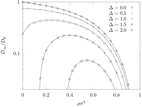

In order to gain a mere phenomenological understanding of the behavior of the system, these observations suggest to look for simple physical arguments explaining the changes in , from which to tentatively infer plausible dynamical evolutions independently of the MCT formalism. At low density, the fluid particles simply tend to occupy the most energetically favorable regions of the random energy landscape. But, because of their excluded-volume interactions, they are progressively forced to occupy less and less favorable ones as density grows. On average, at constant , this leads to a weaker binding of the particles to their preferred locations and an ensuing reduction of the correlations imprinted on the fluid by the random field, which are precisely those measured by . At the dynamical level, for the very same reason, trapping is expected to gradually become less effective on average with increasing density, with an overall acceleration of the dynamics as a result. At moderate and high density, the shape of suggests that, in this regime, the influence of the random energy landscape on the fluid is predominantly indirect and mediated by the excluded-volume interactions. Thus, a reasonable qualitative picture of the system seems to be that of a fluid constrained by the particles most strongly pinned in the wells of the random energy landscape, quite similar to a fluid-matrix system. [53, 54] In such a case, the dynamics of the particles whose motion is hindered by those residing in the lowest energy minima is expected to slow down with increasing density, by a mere crowding effect.
Clearly, the behavior predicted by MCT is fully consistent with these phenomenological considerations. Moreover, experimental evidence has been gathered in favor of a reentrant dynamics of colloids plunged in random light fields. [9] Therefore, it appears that MCT correctly captures the dynamical evolutions of the system at hand, as it does in a number of other cases, [39, 40, 41, 42, 43, 44] despite some obvious limitations, such as the prediction of sharp transitions that might actually be avoided.
The steepness of the line of discontinuous ideal glass transitions delimiting the fluid domain at high density and small-to-moderate disorder strength can also be understood from simple arguments. In this regime, the physics of the system is dominated by excluded-volume interactions, that efficiently screen the smooth random energy landscape. It follows that the disconnected density correlations remain small compared to the connected ones, that essentially reproduce the correlations of the dense fluid without random field. Therefore, the collective quadratic vertices , whose increase is then the main determinant of the discontinuous ideal glass transition, display a rather modest disorder-strength dependence, leading to the one of the density at which dynamical arrest takes place.
We might now proceed to report the behavior of some time-dependent quantities of interest in various regions of the state diagram. The intermediate scattering functions have been thoroughly studied in the case of the fluid-matrix systems, [53, 54] and the generic properties derived there, which actually stem from the overall structure of the MCT equations, hold without change in the present case as well. Therefore, to avoid unnecessary repetition of previous work, we shall concentrate on quantities pertaining to the mean-squared and mean-quartic displacements, which are also those most often reported in experimental and computational studies.

The effect of crossing the diffusion-localization transition line by increasing at fixed density is shown in Fig. 6, where and the critical disorder threshold . As already mentioned, the transition is triggered by the increase of the linear contribution to the self kernel . Therefore, the behavior of the reported quantities is essentially the same as in the noninteracting limit, with alterations in the form of humps at short times. These, whose presence here is due to the coupling of the self and collective dynamics through and whose amplitude increases with density, reflect caging effects readily seen in the curves at . An important aspect of the diffusion-localization transition is its absence of counterpart in the collective dynamics. Indeed, while the self dynamics becomes complex and slow or even arrested, the collective one remains simple and fast; that is, the coherent superposition of the individual anomalous motions results in an essentially featureless relaxation. Although this might seem puzzling at first sight, there is in fact no particular difficulty or inconsistency here, for a number of reasons. On the physical side, as already stressed, it is the decay of the connected ISF which is fast, but the more experimentally relevant full ISF always displays a strictly arrested contribution corresponding to the inhomogeneous equilibrium density profile developed by the fluid in response to its random environment. Moreover, there is no need in principle that the particles can diffuse across the system in order to relax spontaneous thermal density fluctuations about this profile, as measured by the connected ISF. Local processes might be sufficient, and there is no obvious reason why they should develop singularities because, at very large length- and timescales close to , the self dynamics might turn out ergodic or not. Thus, the key point here is the pre-existence of a time-persistent inhomogeneous density profile, representing a very different situation compared to the ideal glass transition of a bulk fluid, where the primary issue is the spontaneous emergence of such a profile. Remarkably, once it is established, one similarly finds that it can sustain localization, either right at the transition, as in one-component systems, [37, 38] or after some delay, in the case of the small component in strongly size-disparate binary mixtures. [94, 95, 96, 97] In the latter case, the secondary diffusion-localization transition in the ideal glass is also seen to leave the collective dynamics unaffected. At a more formal level, within the memory function formalism, one can actually show that the collective and self ISFs are two independent correlation functions, hence they do not need to display the same type of behavior in general. [98] This generic claim is substantiated by studies of simple toy models, in which one precisely observes self dynamics significantly slower and more complex than collective dynamics. [99, 100, 101, 102] Closer to the present system of interest, computer simulations of fluids in random obstacle arrays, for which MCT predicts a similar transition scenario, did evidence strongly contrasting decay patterns and characteristic timescales for self and collective dynamics at moderate-to-strong disorder, [56, 57] in qualitative agreement with the theoretical expectations. [53, 54]
The approach towards the discontinuous ideal glass transition line through an increase of at fixed disorder strength is illustrated in Fig. 7, with and the ideal glass transition density . In this regime, the relaxation is dominated by the slowing-down of the collective dynamics, to which the self one is enslaved via the quadratic term in . Thus, the main observed features are those familiar and well-studied within the MCT for bulk glassforming liquids, [37, 38, 85, 86] that we briefly describe. As glassy arrest sets in, quantities such as the mean-squared displacement develop an increasingly extended plateau reflecting transient localization by caging. This plateau, to which a diverging timescale is attached, is reached according to a power law , and left according to another one , also known as the von Schweidler law. At longer times, a simple diffusive behavior is recovered, with a late-time diffusion coefficient decreasing with density and vanishing at the transition to leading order. The exponents and ( and ) obey
| (36) |
where denotes Euler’s gamma function and the so-called exponent parameter is a definite function of the vertices and non-ergodicity parameters at the transition. In the standard scenario valid for bulk fluids, the von Schweidler law directly crosses over to simple diffusion. This is also the case here, provided is not too large. Otherwise, if is such that the system lies close enough to the diffusion-localization transition line, a transient domain of subdiffusive motion inserts itself between the two regimes, as a consequence of the subcritical but nonnegligible linear term in . The phenomenon is clearly visible in Fig. 7, where an effective subdiffusion exponent can be read off, accompanied by a long time shoulder in .
In all cases, the dynamical signatures of caging appear at earlier times than those of the random energy landscape. The reason directly lies in the significant separation of lengthscales between the typical cage size and the disorder correlation length, as seen in Fig. 8 illustrating the diffusion-localization transition scenario at high density, with and . Clearly, the incipient plateau due to caging lies well below , while subdiffusion starts above. Physically, this simply reflects the fact that a particle has first to escape the cage formed by its neighbors before it can explore and feel the influence of its quenched-random environment.

We finally consider the effect of the disorder correlation length on the dynamical phase diagram, by reporting in Fig. 9 the boundaries of the fluid domain at different ratios . This effect is clearly significant, with a fluid domain extending to larger and larger disorder strengths at high density as increases (note the use of a logarithmic scale on the axis). To a large extent, this result can be understood from the initial growth of the localization threshold with density, which is found to be merely controlled by , hence the large differences in initial slope in the - plane. This is consistent with the physical picture introduced above, in which the low-density behavior of the system was interpreted in terms of a progressive filling of the energetically favorable regions of the random energy landscape. Indeed, since acts as a similarity length for the random field, the density of such regions naturally scales as in space dimension , irrespective of the detailed energetic criteria used for their definition. For not too large values of , the localization threshold reaches a maximum at a density increasing with , beyond which it becomes a decreasing function of . This evolution has been explained above as a transition towards the behavior of a fluid effectively confined by the particles most strongly pinned in the random energy landscape, the maximum resulting from the complex interplay of quenched energetic disorder and excluded-volume interactions. In such a scenario, since the density of deeply trapped particles should also scale as , the effective confinement strength is expected to decrease with increasing , hence a change in the direction of variation of occurring at progressively higher density, as indeed predicted by MCT.

V Summary and conclusion
In this paper, the dynamics of fluids plunged in smooth quenched-random potential energy landscapes has been investigated within the framework of the mode-coupling theory, based on the simple model of the hard-sphere fluid in a statistically homogeneous Gaussian random field. The possible transitions to dynamically arrested states triggered by variations of the disorder strength and/or of the fluid density have been mapped, and the corresponding evolutions of experimentally relevant time-dependent observables and derived quantities characterized.
The quality of the MCT predictions for the system at hand seems to be on a par with what is typically found in applications of this scheme. On the one hand, the theory inescapably outputs dynamical transitions as a consequence of increasing static correlations, despite the fact that this possibility is clearly ruled out in some cases. [30, 32, 33] This means that a sharp transition is systematically predicted, where only a strong dynamical slowing-down likely takes place, which manifests itself in experiments and simulations in the form of non-ergodic behaviors, ageing phenomena, and ensuing deviations from exact equilibrium results (for the late-time diffusion coefficient, for instance). [1, 2, 3, 4, 5, 6, 7, 8, 9] This is exactly the situation met in MCT studies of bulk glassforming liquids, which nevertheless remain quite successful. [45, 46] On the other hand, the theory is found to capture some nontrivial qualitative evolutions of the dynamics, such as its non-monotonicity with fluid density at fixed disorder strength, which has precisely been observed in experiments. [9] The predictions for the local exponent of the mean-squared displacement and for the non-Gaussian parameter in the disorder-dominated regime are also in fair agreement with available simulation data. [26, 27] Altogether, it therefore appears that, notwithstanding its obvious limitations, MCT can be put to good use to gain some insight into the physics of the considered class of systems. Thus, as shown in the previous section, the MCT predictions can be used as a guide in order to devise simple phenomenological arguments allowing one to explain the overall evolutions of the dynamics in mere physical terms.
As a microscopic first-principle approach, the present theory also represents a potentially interesting tool to efficiently investigate how selected changes to the physical characteristics of the system might impact its dynamical behavior. In this respect, the effect of the disorder correlation length has been addressed as an example and clearly shown to be significant, although it does not seem to have been much discussed in the available literature. We believe that this type of exploratory studies could be quite helpful for the design of applications. For instance, in order to develop microfluidic speckle sieves or sorters [12, 13] that evenly work over an as-a-broad-as-possible colloidal density range, our results clearly suggest that random optical fields with a short disorder correlation length should be favored, since they precisely entail a weaker density dependence of particle diffusion. Further refined prescriptions would certainly follow from the extension of the present study to colloidal mixtures, which are by nature the actual systems on which the considered fractionation processes operate. The corresponding theoretical developments are straightforward, but the associated numerical calculations are much more demanding. They are therefore left for future work.
Acknowledgements
We thank Jörg Bewerunge and Stefan Egelhaaf (Düsseldorf, Germany) for useful discussions.
References
- [1] R. D. L. Hanes, C. Dalle-Ferrier, M. Schmiedeberg, M. C. Jenkins and S. U. Egelhaaf, Soft Matter, 2012, 8, 2714–2723.
- [2] R. D. L. Hanes and S. U. Egelhaaf, J. Phys.: Condens. Matter, 2012, 24, 464116.
- [3] F. Evers, C. Zunke, R. Hanes, J. Bewerunge, I. Ladadwa, A. Heuer and S. Egelhaaf, Phys. Rev. E, 2013, 88, 022125.
- [4] F. Evers, R. Hanes, C. Zunke, R. Capellmann, J. Bewerunge, C. Dalle-Ferrier, M. Jenkins, I. Ladadwa, A. Heuer, R. Castañeda-Priego and S. Egelhaaf, Eur. Phys. J. Special Topics, 2013, 222, 2995–3009.
- [5] R. D. L. Hanes, M. Schmiedeberg and S. U. Egelhaaf, Phys. Rev. E, 2013, 88, 062133.
- [6] J. Bewerunge and S. U. Egelhaaf, Phys. Rev. A, 2016, 93, 013806.
- [7] J. Bewerunge, I. Ladadwa, F. Platten, C. Zunke, A. Heuer and S. U. Egelhaaf, Phys. Chem. Chem. Phys., 2016, 18, 18887–18895.
- [8] J. Bewerunge, A. Sengupta, R. F. Capellmann, F. Platten, S. Sengupta and S. U. Egelhaaf, J. Chem. Phys., 2016, 145, 044905.
- [9] J. Bewerunge, Ph.D. thesis, Heinrich-Heine-Universität Düsseldorf, 2016.
- [10] V. G. Shvedov, A. V. Rode, Y. V. Izdebskaya, A. S. Desyatnikov, W. Krolikowski and Y. S. Kivshar, Opt. Express, 2010, 18, 3137–3142.
- [11] V. Shvedov, A. Rode, Y. Izdebskaya, D. Leykam, A. S. Desyatnikov, W. Krolikowski and Y. S. Kivshar, J. Opt., 2010, 12, 124003.
- [12] G. Volpe, G. Volpe and S. Gigan, Sci. Rep., 2014, 4, 3936.
- [13] G. Volpe, L. Kurz, A. Callegari, G. Volpe and S. Gigan, Opt. Express, 2014, 22, 18159–18167.
- [14] E. Pinçe, S. K. P. Velu, A. Callegari, P. Elahi, S. Gigan, G. Volpe and G. Volpe, Nat. Commun., 2016, 7, 10907.
- [15] M. Paoluzzi, R. Di Leonardo, and L. Angelani, J. Phys.: Condens. Matter, 2014, 26, 375101.
- [16] N. Yokoi and Y. Aizu, Opt. Laser Technol., 2017, 90, 226–236.
- [17] S. Havlin and D. Ben-Avraham, Adv. Phys., 1987, 36, 695–798.
- [18] J.-P. Bouchaud and A. Georges, Phys. Rep., 1990, 195, 127–293.
- [19] F. Höfling and T. Franosch, Rep. Prog. Phys., 2013, 76, 046602.
- [20] J. M. Ziman, J. Phys. C: Solid State Phys., 1968, 1, 1532–1538.
- [21] R. Zallen and H. Scher, Phys. Rev. B, 1971, 4, 4471–4479.
- [22] M. B. Isichenko, Rev. Mod. Phys., 1992, 64, 961–1043.
- [23] L. Pezzé, M. R. de Saint-Vincent, T. Bourdel, J.-P. Brantut, B. Allard, T. Plisson, A. Aspect, P. Bouyer and L. Sanchez-Palencia, New J. Phys., 2011, 13, 095015.
- [24] J. Yang and H. Zhao, J. Stat. Mech.: Theory Exp., 2010, 2010, L12001.
- [25] T. O. E. Skinner, S. K. Schnyder, D. G. A. L. Aarts, J. Horbach and R. P. A. Dullens, Phys. Rev. Lett., 2013, 12, 128301.
- [26] S. K. Schnyder, M. Spanner, F. Höfling, T. Franosch and J. Horbach, Soft Matter, 2015, 11, 701–711.
- [27] S. K. Schnyder, T. O. E. Skinner, A. L. Thorneywork, D. G. A. L. Aarts, J. Horbach and R. P. A. Dullens, Phys. Rev. E, 2017, 95, 032602.
- [28] P. G. De Gennes, J. Stat. Phys., 1975, 12, 463–481.
- [29] R. Zwanzig, Proc. Natl. Acad. Sci. U.S.A., 1988, 85, 2029–2030.
- [30] A. De Masi, P. A. Ferrari, S. Goldstein and W. D. Wick, J. Stat. Phys., 1989, 55, 787–855.
- [31] A. K. Chakraborty, D. Bratko and D. Chandler, J. Chem. Phys., 1994, 100, 1528–1541.
- [32] M. W. Deem and D. Chandler, J. Stat. Phys., 1994, 76, 911–927.
- [33] D. S. Dean, I. T. Drummond and R. R. Horgan, J. Stat. Mech.: Theory Exp., 2007, 2007, P07013.
- [34] C. Touya and D. S. Dean, J. Phys. A: Math. Theor., 2007, 40, 919–934.
- [35] D. S. Dean and C. Touya, J. Phys. A: Math. Theor., 2008, 41, 335002.
- [36] S. Banerjee, R. Biswas, K. Seki and B. Bagchi, J. Chem. Phys., 2014, 141, 124105.
- [37] W. Götze, in Liquids, freezing and glass transition, Les Houches 1989, ed. J.-P. Hansen, D. Levesque and J. Zinn-Justin, North Holland, Amsterdam, 1991, pp. 287–503.
- [38] W. Götze, Complex Dynamics of Glass-Forming Liquids – A Mode-Coupling Theory, Oxford University, Oxford, 2009.
- [39] G. Foffi, K. A. Dawson, S. V. Buldyrev, F. Sciortino, E. Zaccarelli and P. Tartaglia, Phys. Rev. E, 2002, 65, 050802.
- [40] E. Zaccarelli, G. Foffi, K. A. Dawson, S. V. Buldyrev, F. Sciortino and P. Tartaglia, Phys. Rev. E, 2002, 66, 041402.
- [41] F. Sciortino, P. Tartaglia and E. Zaccarelli, Phys. Rev. Lett., 2003, 91, 268301.
- [42] K. N. Pham, S. U. Egelhaaf, P. N. Pusey and W. C. K. Poon, Phys. Rev. E, 2004, 69, 011503.
- [43] S. Lang, V. Boţan, M. Oettel, D. Hajnal, T. Franosch and R. Schilling, Phys. Rev. Lett., 2010, 105, 125701.
- [44] S. Mandal, S. Lang, M. Gross, M. Oettel, D. Raabe, T. Franosch and F. Varnik, Nat. Commun., 2014, 5, 4435.
- [45] W. Götze and L. Sjögren, Rep. Prog. Phys., 1992, 55, 241–376.
- [46] W. Götze, J. Phys.: Condens. Matter, 1999, 11, A1–A45.
- [47] W. Götze, E. Leutheusser and S. Yip, Phys. Rev. A, 1981, 23, 2634–2643.
- [48] W. Götze, E. Leutheusser and S. Yip, Phys. Rev. A, 1981, 24, 1008–1015.
- [49] E. Leutheusser, Phys. Rev. A, 1983, 28, 2510–2517.
- [50] G. Szamel, Europhys. Lett., 2004, 65, 498–504.
- [51] V. Krakoviack, Phys. Rev. Lett., 2005, 94, 065703.
- [52] V. Krakoviack, J. Phys.: Condens. Matter, 2005, 17, S3565–S3570.
- [53] V. Krakoviack, Phys. Rev. E, 2007, 75, 031503.
- [54] V. Krakoviack, Phys. Rev. E, 2009, 79, 061501.
- [55] V. Krakoviack, Phys. Rev. E, 2011, 84, 050501(R).
- [56] J. Kurzidim, D. Coslovich and G. Kahl, Phys. Rev. Lett., 2009, 103, 138303.
- [57] J. Kurzidim, D. Coslovich and G. Kahl, Phys. Rev. E, 2010, 82, 041505.
- [58] J. Kurzidim, D. Coslovich and G. Kahl, J. Phys.: Condens. Matter, 2011, 23, 234122.
- [59] K. Kim, K. Miyazaki and S. Saito, EPL, 2009, 88, 36002.
- [60] K. Kim, K. Miyazaki and S. Saito, Eur. Phys. J. Special Topics, 2010, 189, 135–139.
- [61] K. Kim, K. Miyazaki and S. Saito, J. Phys.: Condens. Matter, 2011, 23, 234123.
- [62] M. Spanner, S. K. Schnyder, F. Höfling, T. Voigtmann and T. Franosch, Soft Matter, 2013, 9, 1604–1611.
- [63] M. Alcoutlabi and G. B. McKenna, J. Phys.: Condens. Matter, 2005, 17, R461–R524.
- [64] C. Alba-Simionesco, B. Coasne, G. Dosseh, G. Dudziak, K. E. Gubbins, R. Radhakrishnan and M. Sliwinska-Bartkowiak, J. Phys.: Condens. Matter, 2006, 18, R15–R68.
- [65] R. Richert, Annu. Rev. Phys. Chem., 2011, 62, 65–84.
- [66] M. Spanner, F. Höfling, S. C. Kapfer, K. R. Mecke, G. E. Schröder-Turk and T. Franosch, Phys. Rev. Lett., 2016, 116, 060601.
- [67] G. I. Menon and C. Dasgupta, Phys. Rev. Lett., 1994, 73, 1023–1026.
- [68] F. Thalmann, C. Dasgupta and D. Feinberg, Europhys. Lett., 2000, 50, 54–60.
- [69] R. H. Kraichnan, J. Fluid Mech., 1976, 77, 753–768.
- [70] I. M. Lifshits, S. A. Gredeskul and L. A. Pastur, Introduction to the theory of disordered systems, Wiley, New York, 1988.
- [71] E. M. Chudnovsky and R. Dickman, Phys. Rev. B, 1998, 57, 2724–2727.
- [72] W. Götze, Solid State Commun., 1978, 27, 1393–1395.
- [73] W. Götze, J. Phys. C: Solid State Phys., 1979, 12, 1279–1296.
- [74] W. Götze, P. Prelovšek and P. Wölfle, Solid State Commun., 1979, 30, 369–373.
- [75] W. Götze, Philos. Mag. B, 1981, 43, 219–250.
- [76] E. Leutheusser, Phys. Rev. A, 1983, 28, 1762–1773.
- [77] S. K. Schnyder, F. Höfling, T. Franosch and T. Voigtmann, J. Phys.: Condens. Matter, 2011, 23, 234121.
- [78] J.-P. Hansen and I. R. McDonald, Theory of simple liquids, Second edition, Academic Press, London, 1986.
- [79] G. Grinstein, S.-K. Ma and G. F. Mazenko, Phys. Rev. B, 1977, 15, 258–272.
- [80] S. F. Edwards and P. W. Anderson, J. Phys. F: Metal Phys., 1975, 5, 965–974.
- [81] R. T. Deam and S. F. Edwards, Philos. Trans. R. Soc. A, 1976, 280, 317–353.
- [82] A. Lang, C. N. Likos, M. Watzlawek and H. Löwen, J. Phys.: Condens. Matter, 2000, 12, 5087.
- [83] A. A. Louis, P. G. Bolhuis and J. P. Hansen, Phys. Rev. E, 2000, 62, 7961–7972.
- [84] V. Krakoviack, J.-P. Hansen and A. A. Louis, Phys. Rev. E, 2003, 67, 041801.
- [85] T. Franosch, M. Fuchs, W. Götze, M. R. Mayr and A. P. Singh, Phys. Rev. E, 1997, 55, 7153–7176.
- [86] M. Fuchs, W. Götze and M. R. Mayr, Phys. Rev. E, 1998, 58, 3384–3399.
- [87] M. Fuchs, W. Götze, I. Hofacker and A. Latz, J. Phys.: Condens. Matter, 1991, 3, 5047–5071.
- [88] T. Franosch and W. Götze, J. Phys.: Condens. Matter, 1994, 6, 4807–4822.
- [89] J. Kertész and J. Metzger, J. Phys. A: Math. Gen., 1983, 16, L735–L739.
- [90] A. Kammerer, F. Höfling and T. Franosch, EPL, 2008, 84, 66002.
- [91] T. Franosch, M. Spanner, T. Bauer, G. E. Schröder-Turk and F. Höfling, J. Non-Cryst. Solids, 2011, 357, 472–478.
- [92] M. Spanner, F. Höfling, G. E. Schröder-Turk, K. Mecke and T. Franosch, J. Phys.: Condens. Matter, 2011, 23, 234120.
- [93] T. Franosch, J. Phys. A: Math. Theor., 2014, 47, 325004.
- [94] J. Bosse and J. S. Thakur, Phys. Rev. Lett., 1987, 59, 998.
- [95] J. S. Thakur and J. Bosse, Phys. Rev. A, 1991, 43, 4378–4387.
- [96] J. S. Thakur and J. Bosse, Phys. Rev. A, 1991, 43, 4388–4395.
- [97] T. Voigtmann, EPL, 2011, 96, 36006.
- [98] J.-P. Boon and S. Yip, Molecular hydrodynamics, Dover, New York, 1991.
- [99] D. W. Jepsen, J. Math. Phys., 1965, 6, 405–413.
- [100] W. Dieterich, P. Fulde and I. Peschel, Adv. Phys., 1980, 29, 527–605.
- [101] R. Kutner, Phys. Lett. A, 1981, 81, 239–240.
- [102] K. W. Kehr, R. Kutner and K. Binder, Phys. Rev. B, 1981, 23, 4931–4945.