Collapsar Gamma-Ray Bursts: how the luminosity function dictates the duration distribution

We argue that the (normalized) isotropic GRB luminosity function is the product of the fraction $f$ of successful jets and the engine luminosity function $p(L_{\rm e})$:

where we assumed that the isotropic GRB (radiated) luminosity $L$ is a constant fraction of the isotropic engine luminosity (i.e., $L=\eta L_{\rm e}$), as motivated by the narrow distribution of the $\gamma$-ray efficiency of GRBs (Fan & Piran, 2006; Beniamini et al., 2016, e.g.). Depending on whether $L$ denotes the peak or average burst luminosity, the numerical value of $\eta$ will differ by a factor of $\sim 3$.

Using equations (1), (2), and (9) we find:

where $N_{0}\equiv(a-1)/L_{\min}$, $w=\chi(-\beta+1)<0$ and the break luminosity is defined as:

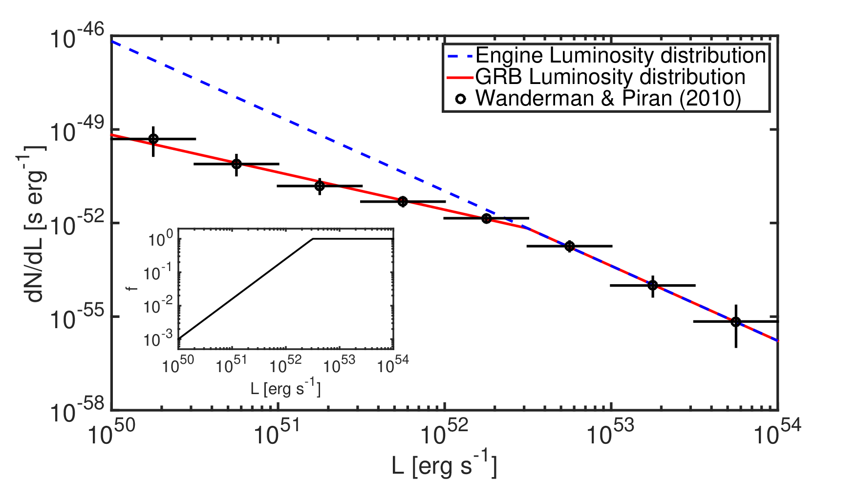
Therefore, a power-law distribution of the central engine luminosity results in a broken power-law distribution of the GRB luminosity function. The break at $L_{\rm br}$ is due to the fact that an increasing fraction of engines with lower luminosities are not able to produce successful GRBs. In contrast, the GRB luminosity function reflects the luminosity function of the central engine for $L>L_{\rm br}$.

Observationally, the GRB luminosity function is, indeed, best described by a broken power law (Wanderman & Piran, 2010; Salvaterra et al., 2012; Pescalli et al., 2016, e.g.):

Comparison of the GRB luminosity function with the predicted one, equation (3.1), allows us to uniquely determine the critical parameters of our model that describe the engine luminosity distribution and its duration:

where we use the standard $Q_{\rm x}=10^{-x}Q$ notation. We present a graphical view of our comparison in Fig. 1 and summarize our results for the two indicative $\chi$ values in Table 1. Interestingly, the minimum engine activity timescale cannot be arbitrarily short for a given $t_{0}$.

The distribution of rest-frame $\gamma$-ray durations of GRBs $t_{\gamma}=t_{\rm e}-t_{\rm b}$ can be calculated using the procedure outlined in Sobacchi et al. (2017). However, we relax their assumption of a fixed $t_{\rm b}$ value by considering a distribution of breakout times as determined by the jet luminosity. In this case, $p_{\gamma}$ is calculated as:

The above equation can be recast in the form:

where $t_{\rm b,max}$ corresponds to the breakout time of the minimum isotropic engine luminosity $L_{\rm e,min}$, see equation (5). The distribution of $\gamma$-ray durations can be analytically derived in two limiting regimes (Bromberg et al., 2012, see also):

1. 1.

   $t_{\gamma}\ll t_{\rm b}$, where $t_{\rm e}\approx t_{\rm b}$. Using also $t_{\rm b,max}\gg t_{\rm e,min}$, equation (24) can be cast in the form:

   $\displaystyle p_{\gamma}(t_{\gamma})\simeq\frac{\beta_{L}(\beta_{L}-\alpha_{L})}{\chi(\beta_{L}-\chi)}t_{\rm b,max}^{-1},$

   (27)

   which is independent of $t_{\gamma}$. For short enough $\gamma$-ray durations, $p_{\gamma}$ is set by the maximum breakout timescale and the power-law indices of the GRB luminosity function.

2. 2.

   $t_{\gamma}\gg t_{\rm b}$, where $t_{\rm e}\approx t_{\gamma}$. Equation (23) then results in:

   $\displaystyle p_{\gamma}(t_{\gamma})\simeq\frac{\beta_{L}(\beta_{L}-\alpha_{L})}{\chi(2\beta_{L}-\alpha_{L})t_{\rm b,max}}\left(\frac{t_{\gamma}}{t_{\rm b,max}}\right)^{-1-\frac{\beta_{L}-\alpha_{L}}{\chi}}.$

   (28)

   In this regime, the distribution of durations reflects the distribution of engine timescales ($p_{\gamma}\propto t_{\gamma}^{-\beta}$), in agreement with previous works (Bromberg et al., 2012; Sobacchi et al., 2017). However, in our study, the power-law slope of the engine time distribution $\beta$ is not a free parameter to be determined by comparison to the GRB duration distribution. It is instead uniquely determined by the power-law slopes of the GRB luminosity function (i.e. $\alpha_{L},\beta_{L}$) and $\chi$ and can be used as a test of the model against the observed duration distribution of GRBs.

For a specific jet propagation theory ($\chi$ value) and GRB luminosity function, the only free parameter which enters the calculation of $p_{\gamma}(t_{\gamma})$ is the maximum breakout time. This affects both the “plateau” and the turnover of the distribution $p_{\gamma}$, see equations (27) and (28). Thus, $t_{\rm b,max}$ can be determined by fitting the model, equation (24), to the duration distribution of collapsar GRBs.

To derive the observed GRB duration distribution, we used the $T_{90}$²² 2 This is a measure of the GRB duration and is defined as the time interval during which 90 per cent of the photon counts have been detected (Kouveliotou et al., 1993). value of 1066 GRBs detected by the Swift satellite during the period of 2004 -- 2017³³ 3 https://swift.gsfc.nasa.gov/archive/grb_table/. Redshift information is available only for $\sim 1/3$ of the sample, with a median redshift of $z\simeq 1.7$. This was adopted as the typical redshift of the entire Swift sample in order to construct the histogram of rest-frame $\gamma$-ray durations as $t_{90}=T_{90}/(1+z)$.

The normalized histogram of $t_{90}$ of all Swift GRBs is plotted in Fig. 2 with a black line. The corresponding histogram of Swift GRBs with measured redshifts is also shown for comparison (orange line). Overall, the two histograms are qualitatively similar with the main differences appearing at short durations. Regardless, GRBs with $t_{90}\lesssim 0.3$ s (i.e., short GRBs) do not have a collapsar origin and are neglected in this study. Overplotted as coloured curves are our model predictions with $t_{\rm b,max}\simeq 69$ s for $\chi=1/3$ and $t_{\rm b,max}\simeq 47$ s for $\chi=1/2$ (see also Table 1). Both provide very good quantitative descriptions to the collapsar GRB duration distribution. In fact, the plateau of the duration distribution is expected to be similar for models with the same product of $\chi$ and $t_{\rm b,max}$, as long as $\beta_{\rm L}\gg\chi$. More specifically, $p_{\gamma}\propto(\chi t_{\rm b,max})^{-1}$ at short enough durations, see equation (27). From the “fit” to the duration distributions with $\chi=1/3$ and $\chi=1/2$ we find $\chi t_{\rm b,max}\approx T_{\max}$ where $T_{\max}\simeq 23$ s.

A timescale of $\sim 60$ s – beyond which the duration distribution turns into a steep power law – is also found by Sobacchi et al. (2017). The authors associate this timescale with a single breakout time assumed for all GRBs, whereas in our framework it is clearly related to the maximum breakout time. In addition, Sobacchi et al. (2017) fit their data in order to derive $\beta$, whereas in our model $\beta$ is uniquely determined by the GRB luminosity function and $\chi$ – see equation (28). A fit to the data is not guaranteed in our model. For instance, the observed $p_{\gamma}$ distribution cannot be explained by luminosity functions with $\beta_{L}-\alpha_{L}<1$ for $\chi$ in the range $1/3-1/2$, as motivated by theory (Bromberg et al., 2011a; Lazzati et al., 2012).

The maximum breakout time inferred from the observed GRB duration distribution can also be translated to a constraint between $t_{0}$ and a minimum luminosity for a given $\chi$ value. Using $\chi t_{\rm b,max}\approx T_{\max}$ together with equation (5), we find:

In our analysis we assumed that the Swift GRB sample is complete with respect to the observed burst duration. In other words, for a fixed luminosity the detection of the burst does not depend on its duration. This is a simplifying assumption, for the minimum detectable flux of a GRB depends upon the exposure time $T$ as $T^{-1/2}$ (Baumgartner et al., 2013; Lien et al., 2016). For GRBs, the maximum exposure time is set by their duration. For simplicity, let us identify $T$ as the observed duration $T_{90}$. This implies that the flux limit for detection is higher for GRBs with shorter duration. Indeed, there is lack of luminous and short bursts (i.e., $L_{\rm iso}>10^{52}$ erg s^-1 and $T_{90}<2$ s) in the third Swift/BAT GRB catalog (see Fig. 25 in Lien et al., 2016). This can be the result of a genuine lack of GRBs with these properties or of unavailable redshift measurements. Regardless, these results suggest that the Swift/BAT sample is complete with respect to burst duration for long GRBs. Therefore, we do not expect our main conclusions to depend strongly on this assumption.

For a distribution of breakout times we showed that the only free parameter that controls $p_{\gamma}(t_{\gamma})$ (both the plateau and position of the break) is the maximum breakout time. This, in turn, depends upon $t_{0}$ and $L_{\min}$, see equations (5) and (29). Here, $L_{\min}$ should not be interpreted as the intrinsic GRB minimum luminosity. In fact, the GRB sample becomes progressively less complete for lower isotropic GRB luminosities (Wanderman & Piran, 2010, e.g.,). Thus, the duration distribution probes GRBs with isotropic luminosities down to an “effective” minimum luminosity $L_{\rm eff}$. Substitution of $L_{\rm eff}\simeq 10^{51}$ erg s^-1 to equation (29) leads to a conservative constraint:

which translates to $t_{0}\sim 150$ s for all $\chi$ values in the range $1/3-1/2$ and $T_{\max}\sim 23$ s. Values of $t_{0}\gg 20$ s cannot be easily reconciled with the scenario of jet propagation through a compact progenitor, because of the weak dependence that $t_{0}$ has on stellar properties (Bromberg et al., 2011a; Bromberg et al., 2012, see). Our analysis suggests the presence of an extended low-mass envelope surrounding the GRB progenitor, as concluded independently by Sobacchi et al. (2017). The weak dependence of the breakout time on $L_{\rm eff}$ makes this conclusion quite robust.

Assuming a common $t_{0}\sim 150$ s for all GRB collapsars, we can further predict that the duration distribution will extend towards longer durations (i.e., larger $t_{\rm b,max}$ and $T_{\max}$) as the sample becomes more complete at lower luminosities thanks to more sensitive future missions. Falsification of this prediction would provide indirect evidence for a distribution of $t_{0}$ among GRB progenitors, which lies beyond the scope of this paper.

We next examine the energetics of central engines and their potential in powering a supernova explosion. All engines with $L_{\rm e}>L_{\rm e,*}\equiv\eta^{-1}L_{*}$ produce successful GRBs. The associated energy deposited to the stellar envelope by successful engines is

where $f_{\rm b}=0.01\ f_{\rm b,-2}$ is the jet beaming fraction and

The minimum engine timescale $t_{\rm e,min}$ is given by equation (22). Failed jets can also inject a considerable amount of energy to the stellar envelope. For $L_{\rm e,min}\leq L_{\rm e}\leq L_{\rm e,*}$ the engine activity timescale $t_{\rm e}$ lies between $t_{\rm b,max}$ and $t_{\rm e,min}$. The latter is still a good proxy for the average $t_{\rm e}$ in the range of $[t_{\rm e,min},t_{\rm b,max}]$ because of the steepness of $p_{\rm e}(t_{\rm e})$. The energy of a failed GRB engine is then given by

Figure 3 presents the beaming-corrected energy, $E_{\rm e}$, of successful and failed engines (see equations (31) and (33), respectively) as a function of $L_{\rm e}$ for $\chi=1/3-1/2$ and $t_{0}=150$ s. For a typical GRB engine (i.e., $L_{\rm e}=L_{\rm e,*}$), we find

for $\chi=1/3-1/2$. This is comparable to the kinetic energy inferred in SNe associated to long GRBs (Hjorth & Bloom, 2012, e.g.,) and provides further support that GRB-SNe are jet-driven (Hjorth, 2013, e.g.,). Failed jets that inject $\sim 10^{51}$ erg (1 foe) to the stellar envelope – an energy comparable to the binding energy of the stellar envelope and the typical kinetic energy of core-collapse SNe – could facilitate the explosion mechanism in these SNe (Sobacchi et al., 2017; Piran et al., 2017), but they are not expected to drive mildly relativistic SNe ejecta (Soderberg et al., 2010, see e.g.). The isotropic engine luminosity in this case is $L_{\rm e,foe}=10^{52}\ E_{\rm e,51}f_{\rm b,-2}^{-1}t_{\rm e,min,1}^{-1}$ erg s^-1.

Jets can deposit a significant energy into the stellar envelope on timescales of tens of seconds (i.e., $t\gtrsim t_{\rm e,min}$), but it is unlikely that they can produce the necessary mass of radioactive ⁵⁶Ni to partially power the optical light curve of core-collapse SNe (Hamuy, 2003; Müller et al., 2017, i.e., $\sim 0.02\,M_{☉}-0.2\,M_{☉}$,). Being a by-product of the explosive silicon burning process, ⁵⁶Ni can be synthesized under specific temperature and density conditions (Woosley et al., 1973; Woosley & Weaver, 1995; Jerkstrand et al., 2015, e.g.), which cannot be easily met once the ejecta has expanded far from the central engine.

Although failed jets cannot be the sole mechanism that drives the SN explosion, a picture emerges where they may be an important component of this process (Lazzati et al., 2012; Sobacchi et al., 2017; Piran et al., 2017, e.g.). The limitation on jet-driven explosions stems from the energetic requirement of injecting $\sim 10^{51}$ erg and not from a lack of engines at these lower luminosities (see dash-dotted line in Fig. 3). The number of failed GRB engines with $L_{\rm e}<L_{\rm e,*}$ can be written as $N_{\rm f}(L_{\rm e})\approx\left(L_{\rm e}/L_{\rm e,*}\right)^{-\beta_{L}}$, where a normalization of one engine at luminosity $L_{\rm e,*}$ was assumed. The true rate of failed engines capable of injecting $\sim 10^{51}$ erg at typical $\hat{z}=2$ can be then estimated as:

where $R_{\rm GRB}(\hat{z})\approx 10$ Gpc^-3 yr^-1 is the observed (i.e., uncorrected for beaming) collapsar GRB rate (Wanderman & Piran, 2010; Sobacchi et al., 2017). We also used $\beta_{L}=1.4$ and assumed a redshift independent engine luminosity function. Interestingly, this order-of-magnitude prediction is consistent with inferred rates of Type Ib/c SNe at $\hat{z}\sim 2$ (Dahlen et al., 2004; Dahlen et al., 2012; Cappellaro et al., 2015; Strolger et al., 2015, e.g.) suggesting an active role of the central engine in all Ib/c SNe (Sobacchi et al., 2017; Bear et al., 2017, see also).

Our results, although consistent with those by Sobacchi et al. (2017), are derived with a very different method. The number and energetics of our failed jets, as well as the minimum engine timescale are naturally obtained by matching the distribution of successful engines with the GRB luminosity function, instead of relying on an extrapolation of the central engine duration distribution to an (almost) arbitrary value.

Our analysis was performed independently of the nature of the GRB central engine, which can be either a newly born black hole or a magnetar (i.e., a rapidly spinning highly magnetized neutron star), see, e.g., Kumar & Zhang (2015) for a review on GRB central engines. Our predictions for the energetics of central engines are summarized in Fig. 3 and can be used to constrain their nature. We showed that the beaming-corrected energy of a typical GRB engine that is active for $t_{\rm e,min}\sim 10$ s is a few $\times 10^{52}$ erg, see also equation (34). This might be already in tension with the magnetar scenario, although recent studies cast doubt on previous estimates on the maximum energy extractable in the magnetar model (Metzger et al., 2015). In addition, the distributions of the engine duration and luminosity are expected to differ between models of the central engine. In the magnetar scenario, for example, where the luminosity and duration of the engine depend both on the magnetic field and spin period of the magnetar (e.g., Usov, 1992), the distributions of $L_{\rm e}$ and $t_{\rm e}$ will be correlated. A careful comparison of our model predictions against several observational constraints, such as the GRB distribution on the $L-T_{90}$ plane, will be the subject of a follow-up study.

References

- Baumgartner et al. (2013) Baumgartner W. H., Tueller J., Markwardt C. B., Skinner G. K., Barthelmy S., Mushotzky R. F., Evans P. A., Gehrels N., 2013, ApJS, 207, 19
- Bear et al. (2017) Bear E., Grichener A., Soker N., 2017, preprint, (arXiv:1706.00003)
- Beniamini et al. (2016) Beniamini P., Nava L., Piran T., 2016, MNRAS, 461, 51
- Bromberg et al. (2011a) Bromberg O., Nakar E., Piran T., 2011a, ApJ, 739, L55
- Bromberg et al. (2011b) Bromberg O., Nakar E., Piran T., Sari R., 2011b, ApJ, 740, 100
- Bromberg et al. (2012) Bromberg O., Nakar E., Piran T., Sari R., 2012, ApJ, 749, 110
- Bromberg et al. (2013) Bromberg O., Nakar E., Piran T., Sari R., 2013, ApJ, 764, 179
- Cappellaro et al. (2015) Cappellaro E., et al., 2015, A&A, 584, A62
- Dahlen et al. (2004) Dahlen T., et al., 2004, ApJ, 613, 189
- Dahlen et al. (2012) Dahlen T., Strolger L.-G., Riess A. G., Mattila S., Kankare E., Mobasher B., 2012, ApJ, 757, 70
- Fan & Piran (2006) Fan Y., Piran T., 2006, MNRAS, 369, 197
- Hamuy (2003) Hamuy M., 2003, ApJ, 582, 905
- Hjorth (2013) Hjorth J., 2013, Philosophical Transactions of the Royal Society of London Series A, 371, 20120275
- Hjorth & Bloom (2012) Hjorth J., Bloom J. S., 2012, The Gamma-Ray Burst - Supernova Connection. pp 169–190
- Jerkstrand et al. (2015) Jerkstrand A., et al., 2015, The Astrophysical Journal, 807, 110
- Kouveliotou et al. (1993) Kouveliotou C., Meegan C. A., Fishman G. J., Bhat N. P., Briggs M. S., Koshut T. M., Paciesas W. S., Pendleton G. N., 1993, ApJ, 413, L101
- Kumar & Zhang (2015) Kumar P., Zhang B., 2015, Phys. Rep., 561, 1
- Lazzati et al. (2012) Lazzati D., Morsony B. J., Blackwell C. H., Begelman M. C., 2012, ApJ, 750, 68
- Lien et al. (2016) Lien A., et al., 2016, ApJ, 829, 7
- MacFadyen & Woosley (1999) MacFadyen A. I., Woosley S. E., 1999, ApJ, 524, 262
- Margutti et al. (2014) Margutti R., et al., 2014, ApJ, 797, 107
- Metzger et al. (2015) Metzger B. D., Margalit B., Kasen D., Quataert E., 2015, MNRAS, 454, 3311
- Mizuta & Aloy (2009) Mizuta A., Aloy M. A., 2009, The Astrophysical Journal, 699, 1261
- Morsony et al. (2007) Morsony B. J., Lazzati D., Begelman M. C., 2007, The Astrophysical Journal, 665, 569
- Müller et al. (2017) Müller T., Prieto J. L., Pejcha O., Clocchiatti A., 2017, ApJ, 841, 127
- Nakar (2015) Nakar E., 2015, ApJ, 807, 172
- Paczyński (1998) Paczyński B., 1998, ApJ, 494, L45
- Pescalli et al. (2016) Pescalli A., et al., 2016, A&A, 587, A40
- Piran et al. (2017) Piran T., Nakar E., Mazzali P., Pian E., 2017, preprint, (arXiv:1704.08298)
- Salvaterra et al. (2012) Salvaterra R., et al., 2012, ApJ, 749, 68
- Sobacchi et al. (2017) Sobacchi E., Granot J., Bromberg O., Sormani M. C., 2017, preprint, (arXiv:1705.00281)
- Soderberg et al. (2010) Soderberg A. M., et al., 2010, Nature, 463, 513
- Soker (2016) Soker N., 2016, New Astron. Rev., 75, 1
- Strolger et al. (2015) Strolger L.-G., et al., 2015, ApJ, 813, 93
- Usov (1992) Usov V. V., 1992, Nature, 357, 472
- Wanderman & Piran (2010) Wanderman D., Piran T., 2010, MNRAS, 406, 1944
- Woosley & Weaver (1995) Woosley S. E., Weaver T. A., 1995, ApJS, 101, 181
- Woosley et al. (1973) Woosley S. E., Arnett W. D., Clayton D. D., 1973, ApJS, 26, 231
- Zhang et al. (2003) Zhang W., Woosley S. E., MacFadyen A. I., 2003, The Astrophysical Journal, 586, 356