Reduced energy consumption in stirred vessels
by means of fractal impellers
S. Başbuğ, G. Papadakis and J. C. Vassilicos
Department of Aeronautics, Imperial College London, SW7 2AZ London, UK
Earlier studies[1, 2] have shown that the power consumption of an unbaffled stirred vessel decreases significantly when the regular blades are replaced by fractal ones. In this paper, the physical explanation for this reduction is investigated using Direct Numerical Simulations at . The gaps around the fractal blade perimeter create jets that penetrate inside the recirculation zone in the wake and break up the trailing vortices into smaller ones. This affects the time-average recirculation pattern on the suction side. The volume of the separation region is smaller in the wake of the fractal blades. The lower torque of the fractal impeller is equivalent to a decreased transport of angular momentum; this difference stems from the reduced turbulent transport induced by the smaller trailing vortices. The major difference in the turbulent dissipation is seen in the vicinity of trailing vortices, due to fluctuations of velocity gradients at relatively low frequencies.
Keywords: DNS, trailing vortices, radial impeller, power consumption, pressure coefficient.
Introduction
Stirred vessels are employed in a wide range of mixing applications in the chemical, pharmaceutical and process industries.[3] Reducing power consumption and/or increasing mixing quality improves process efficiency. Modification of blade design has been considered as a means to achieve this objective. Indeed this has been the subject of extensive research in the past decades, [4, 5, 6, 7, 8, 9] but these efforts yielded only modest improvements.[8, 9]
Steiros et al.[1] continued work in this direction and proposed a promising new impeller design. They introduced blades of fractal shape and compared their performance to that of regular blades. The application of fractal geometry to blade design was inspired by results obtained in other areas over the past ten years, summarized by the aforementioned authors[1] and in our previous paper.[2] More specifically, Steiros et al.[1] performed shaft torque measurements to determine the power consumption of four-bladed radial impellers in an unbaffled tank at , where is based on the rotational speed , impeller diameter and kinematic viscosity of the fluid . Their results demonstrated that the fractal-1 impeller, that uses blades with one fractal iteration (seen in Figure 3(b)) has reduced power consumption compared to the impeller with regular blades (seen in Figure 3(a)). When the fractal-2 impeller was employed (with two fractal iterations, see Figure 2 in Steiros et al.[1]), this difference increased to . The authors also measured the pressure distribution on both sides of the blades using pressure transducers. They found that the center of pressure for a fractal blade is located radially further away from the shaft compared to a regular one. Consequently it was shown that the decreased torque on the fractal blade is due to the lower net pressure force applied onto the blade and not due to the reduced moment arm length. Since both types of blades have equal frontal area by construction, it was concluded that the fractal blade has a lower drag coefficient. Furthermore, they tested a two-bladed impeller, where one regular and one fractal blade were mounted 90° apart. They conducted experiments for both rotational directions, whereby the regular blade was immersed in the wake of the fractal blade and vice versa. They measured exactly the same torque in both experiments. This finding suggests that the wake interaction was not the reason for the reduced drag coefficient of a fractal blade. However, their results did not identify and explain clearly the mechanism which leads to the reduced torque.
In the present study, we use Direct Numerical Simulations (DNS) to conduct a detailed analysis of the flows around both impeller types. We aim to answer the following open questions: Why does the fractal impeller require reduced torque and power consumption with respect to a regular one with equal frontal area? How is this related to the flow patterns in the wake? The physical understanding from such an investigation can lead to further improvements in impeller design in the future.
We have performed DNS of the flow field inside an unbaffled stirred vessel with four-bladed radial impellers at and . The DNS approach produced high fidelity, well-resolved data of velocity and pressure in space and time. Such time-accurate and comprehensive database allows a detailed analysis of the wake flow patterns, and their effect on the pressure field around the impeller and the distribution of energy dissipation in the whole tank. There are few other DNS studies of the flow in baffled[10] and unbaffled[11] stirred tanks, but with different goals to those of the present work.
The remainder of this paper is organized as follows: In the following section, we introduce the flow configuration and describe briefly the numerical methodology employed. This is followed by a comparison between experimental and numerical results for validation, and a comparative summary of the power consumption. The pressure distribution on regular and fractal blades and its relation to the flow is presented and analysed. Differences in transport of angular momentum and in energy dissipation between the two impeller types are investigated. We close the paper with a summary and main conclusions.
Flow configurations examined
The stirred tank used in the present study has a cylindrical geometry of equal height and diameter, with a four-bladed impeller located at the mid-height. Figures 1(a) and 1(b) show vertical and horizontal views of the vessel and the impeller. The blade height and blade thickness are and of the tank diameter, respectively. Two types of impeller blades with equal frontal area were employed in the present work, referred to below as regular and fractal blades, illustrated in Figures 3(a) and 3(b) respectively. These blades are the same ones used in our previous DNS study.[2] They also match some of the blades in the experimental study of Steiros et al.[1]
As seen in Figure 3, the radius of the fractal impeller is not uniform. The furthest tip is located at , where is the constant radius of the regular impeller. For normalization purposes, the dimensions of the regular impeller are used throughout the paper.
Numerical methodology
The incompressible in-house code “Pantarhei” was used to obtain the DNS results presented in the paper. The code is based on the finite-volume method and was previously employed for DNS of the flow around an airfoil,[12] the flow past a single square grid-element[13] and the flow in an unbaffled stirred vessel.[2] More details can be found in the latter reference which deals with the same configuration as the present study. The Navier-Stokes equations were solved in a rotating reference frame, fixed to the impeller. In this frame, the momentum equations take the form:
| (1) |
where is the instantaneous velocity vector in the rotating frame, is the viscous stress tensor and denotes the angular velocity of the frame. The origin of the coordinate system is located on the impeller axis at the mid-height of the vessel. The position vector with respect to the origin is denoted by . Vector points in the axial direction and has magnitude . The last two terms of Equation 1 represent the centrifugal and Coriolis forces respectively, and were treated as source terms. A prescribed velocity (equal to , where is the radial distance of a wall point to the axis of the vessel) was imposed on all external walls to represent the relative motion with respect to the impeller. The top boundary was also treated as a solid wall, hence free-surface depression was not considered. In Basbug et al.[2] the results of the code in terms of mean and rms velocities were validated against those of Verzicco et al.[11] and Dong et al.[14]
The flow inside the vessel was simulated at two Reynolds numbers, and . For , the grids consisted of and cells for the regular and fractal impellers, respectively. For , we used and cells, respectively. Details about the grid resolution and convergence study can be found in Basbug et al.[2]
Comparison with experimental results
The numerical results at are compared with data acquired by means of phase-locked planar particle image velocimetry (PIV) at . The experiments were performed using blades of the same shape in an unbaffled tank of the same dimensions. The only difference was that the tank was hexagonal instead of cylindrical, but this difference is not expected to affect the results in the near impeller region. More details on the stirred tank setup and experimental technique can be found in Steiros et al.[15]
The instantaneous velocity vector in the absolute reference frame is denoted by and can be decomposed in mean and fluctuating components as ; the same decomposition is applied to as well later in the text. The azimuthal velocity component was not accessible in the aforementioned experiment. Using the radial and axial velocity fluctuations only, and respectively, the turbulence intensity () is defined as follows:
| (2) |
where angular brackets represent the time-averaging operation and is the blade tip velocity. Profiles of obtained numerically and experimentally are compared in Figure 2 along a radial line 30° behind the regular impeller, at an axial position where the center of the upper trailing vortex core is located, where the mean azimuthal vorticity, i.e. , is at its highest. This point is preferred to a fixed axial coordinate since the location of vortex cores depends on .
As seen in Figure 2, the two curves are in qualitative agreement despite the large difference in (two orders of magnitude). The peaks of indicate the locations of the vortex cores and their radial positions (between ) are in agreement. A second, but less prominent peak, appears around due to the wake of the preceding blade, and in this region the curves collapse. Yoon et al.[16] investigated the Reynolds number scaling of the flow in an unbaffled tank stirred with a Rushton turbine using phase-locked stereoscopic PIV measurements for a range of values between and . They reported that the vortex core diameter decreases as rises. The results shown in Figure 2 are in accordance with their observation, the peaks of become sharper and narrower with increasing .
Raju et al.[17] conducted a similar study (using the same configuration as Yoon et al.[16]) and measured the rms of the components of in a plane normal to the radial direction close to a blade tip. They reported that the rms values (averaged over the measurement plane) decrease slowly with increasing , from to ca. . For larger , the rms values remained constant. The experimental results presented in Figure 2 were obtained for a higher than the aforementioned threshold for -independence. The moderately higher level of at is also in accordance with the findings of Raju et al.[17] In conclusion, the present numerical results are in qualitative agreement with experimental findings. The observed discrepancies are attributed to the large difference in Reynolds number.
Power consumption for the two blade types
The power, , drawn by the impeller can be computed using two different approaches. In the first approach, the torque of the pressure and skin friction forces applied on the impeller and shaft surfaces is integrated to compute the total impeller torque, , which is then multiplied with the angular velocity, so . In the second approach, the dissipation of the total kinetic energy, , is integrated over the tank volume. The dissipation is defined as , where is the strain-rate tensor, . This definition includes the contributions of both the turbulent dissipation and the dissipation due to the mean velocity gradients. Since the tank is a closed volume, the source and sink of energy must balance on average. Therefore, the power injected by the impeller must equal the total dissipation, when both quantities are averaged over a long period of time.
The power number is defined as . Table I provides the values of based on the power input of the impeller and the volume integral of dissipation, averaged over 80 revolutions for and for 120 revolutions for (also the other mean quantities presented in this paper were averaged for the same duration as stated for at the corresponding ). The observed imbalance between the two approaches varies between and . It was also shown in the previous study[2] that the torque applied by the impeller is in very good agreement with the integral torque applied by the tank walls, with discrepancies between and . This suggests that the approach based on the impeller torque is a more reliable method for the calculation of the power consumption compared to the volume integration of dissipation.
| Blade type, Re | Reg., | Fr., | Reg., | Fr., |
|---|---|---|---|---|
| Impeller power | ||||
| Integral dissipation | ||||
| Imbalance |
The results on the impeller power show that the power consumption is equal for both types of impellers at , with (see Table I). In fact, the contribution of the shear stress to the impeller torque is only for the regular impeller, whereas it is for the fractal impeller at this . This difference is expected because a fractal blade has ca. twice the perimeter length of a regular blade, as seen in Figure 3. If only pressure forces were taken into account, we would obtain a lower with the fractal impeller by ca. , which is compensated by the increased skin friction drag.
At , the contribution of the shear stress is an order of magnitude lower than at , and it therefore has no significant influence on the power consumption. Also at , the numerical results suggest a power reduction of ca. when the regular blades are replaced with fractal blades. This difference is in accordance with the aforementioned experimental results[1] obtained at much higher . In the following sections, we endeavour to provide a physical explanation for this behaviour, mainly focusing on the results at . In order to arrive at a coherent picture, we consider the pressure distribution over the blades, the transport of angular momentum and how it is affected by vortical wake structures, the distribution of dissipation in the wake and the whole vessel, as well as the frequency content of dissipation.
Pressure distribution on blade surfaces
Considering that both regular and fractal impellers rotate with the same angular velocity, any difference in the power is a consequence of a different torque on the impeller. Therefore, we start the analysis with an investigation of pressure distribution on the blade surfaces. The time-averaged pressure difference between the suction and pressure sides is normalized to define a local pressure coefficient, , as follows:
| (3) |
The distribution of over the blades surface is illustrated in Figure 3, and qualitatively it agrees well with the experimental results.[1] The maximum value for the regular blade is close to , whereas for the fractal blade it reaches up to . In the experiments[1] with , the maximum value was less than . It is expected that this quantity will be lower at higher , because is lower as well. The radial positions of maxima are denoted with vertical dashed lines in Figure 3. These are located at and for the regular and fractal blades, respectively. From the distributions reported in the aforementioned experimental study, it appears that the maxima are located in similar positions, but the exact locations were not stated.


From the surface integral of , the drag coefficient can be computed as . The values of from the present DNS study and the experiments[1] at are listed in Table II. Note that is based on pressure forces only, i.e. viscous forces are excluded. The center of pressure, , is also included in Table II. It is defined as the net torque divided by the net force applied on the blade, and it is normalized with the impeller radius, . As expected, decreases with the increasing , a behaviour similar to that of . Moreover, moves radially further from the axis as rises. At every , the fractal blade has a lower than the regular blade. At , the larger value of and the more significant viscous forces on the fractal blade compensate for the lower , so that both blades apply the same torque on the fluid. At the higher numbers, the reduced pressure drag force on the fractal impeller is the dominant factor that explains the lower torque with respect to the regular impeller.
| Blade type | Reg. | Fr. | Reg. | Fr. | Reg. | Fr. |
|---|---|---|---|---|---|---|
| Re | (exp.) | (exp.) | ||||
In order to gain more insight on the observed pressure distributions, we turn our attention to the velocity fields around the blades. Figure 4a shows the mean azimuthal velocity profiles acquired along two radial lines, at 10° upstream of the pressure side and 10° downstream of the suction side (as depicted in Figure 4b). These profiles were obtained at the mid-height of the tank, in the relative reference frame, at . Since the impeller rotation is in the positive azimuthal direction, as indicated with an arrow in Figure 4b, the relative azimuthal velocities () will have negative values on the pressure side along the entire profile. For the radial positions up to half of the blade radius (), the velocity magnitudes are less than of for both types of blades on both sides. This explains why values are very low on the inner half of the blades, as seen in Figure 3.

The profiles of on the pressure sides of both blades collapse (solid lines in Figure 4a). This is consistent with the results of experiments[1] using a two bladed impeller, where one regular and one fractal blade are mounted 90° apart. The measured torque was the same when the impeller rotated in either direction, immersing the regular or fractal blade in the wake of the other. This led to the conclusion that the wake interaction is not the reason of the reduced drag coefficient of a fractal blade. Here we elaborate further and show that this is because the upstream velocity profiles are almost independent of the type of the preceding blade. On the other hand, the velocities downstream of the blades are significantly different (dashed lines in figure 4a). This may seem contradictory if one expects that the downstream profile of a blade must interact with the following blade. In our observation, there is a strong radial jet along the suction side of the blades which carries the fluid in the wake radially away. The part of the flow field immediately upstream of the blade is mainly advected axially from the top and bottom of the tank towards the mid-height along the shaft, before interacting with the pressure side. Therefore, the profiles on the pressure side are strongly affected by the angular momentum of the fluid that is in the bulk of the flow far from the impeller. If the bulk flow had higher angular momentum (i.e. higher positive azimuthal velocity in absolute frame, as it is observed at increased [18]), then the profiles of on the pressure side would have a smaller magnitude (i.e. lower velocity relative to the blade). This would lead to a weaker stagnation on the pressure side and a lower drag coefficient, as it is seen in Table II for growing .
We define the flow separation zone in the wake of a blade as the region where is positive, i.e. towards the blade suction side (see Figure 4b). This region extends until about in the wake of the regular impeller (blue dashed line in Figure 4a). Moreover, the magnitude of reaches a maximum value of . On the other hand, in the wake of the fractal impeller becomes negative again around and the maximum magnitude is only , indicating a smaller and weaker separation zone.


The separation zone as defined above is illustrated in Figures 5a and 5c in a three dimensional view in the wakes of regular and fractal blades, respectively. Taking all four blades into account, the size of the separated region is and , respectively, of the impeller swept volume (). The larger separating zone in the wake of a regular blade (by about ) causes a lower pressure on the suction side, resulting in a higher form drag. At first sight, this finding seems to contradict the results of Nedić et al.[19] who performed wind tunnel experiments with square and fractal plates placed normal to an incoming flow. The shapes of the plates were similar to the blades used in the present study. In this flow setting, they measured larger values for the fractal plates compared to the orthogonal plates. However, this flow setting is different to the one examined in the present paper. While the front stagnation flow patterns may be qualitatively similar, the wakes have markedly different behaviour. The rotation of the blade creates a strong radial jet, that is absent when the object is placed normal to the flow. The presence of the radial jet changes entirely the wake properties, resulting in different trends in the values.
Figures 5b and d illustrate contours of in a cross section of the separation zones at the tank mid-height. The dark red colour indicates the location with the highest . This location is radially further away from the axis for the regular blade compared to the fractal blade, and matches with the radial location where the highest was observed in Figure 3a, at . On the other hand, the fractal blade has the highest near the tip of the blade, as seen in Figure 3b, which does not coincide with the location of the strongest separation. This can be explained as follows: Since the tip of the fractal blade extends radially further (up to ) than the tip of the regular blade (up to ), the approaching relative velocity is higher, leading to higher stagnation pressure on the pressure side. This is the dominant factor that determines the location of highest for the fractal blade.


In order to analyse further the mechanism that leads to a smaller separation region in the suction side of the fractal blades, the streamlines around both types of blades are illustrated in Figure 6. To generate the streamlines, the radial velocity component is subtracted from the mean flow field and only the mean axial and azimuthal components are used. In other words, the effect of radial jet is not illustrated in these figures. The streamlines are coloured according to . As seen in Figure 6 a), the flow passing along the upper and lower edges of the regular blade recirculates in the wake and turns towards the suction side. With the influence of the radial jet along the suction side of the blade, the recirculating fluid is carried towards the blade tip, resulting in a spiraling motion that gives rise to the trailing vortex pair.
In the case of the fractal impeller, the concave parts of the blade perimeter allow the upcoming fluid with high azimuthal velocity, hence high momentum, to enter into the recirculation region formed in the wake. The jets penetrate and brake the two large recirculation zones, leading to multiple smaller recirculation zones.
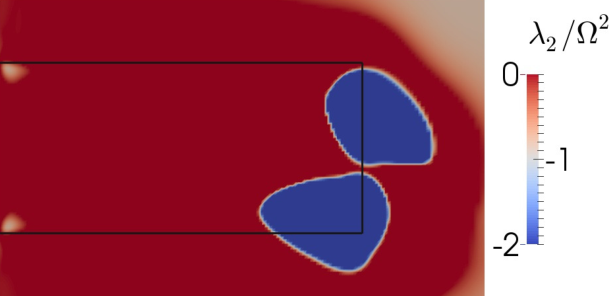
This has a profound influence on the coherent trailing vortex structures present in the wake of the blades. Vortex cores can be visualised with the help of the -criterion introduced by Jeong and Hussein.[20] In this criterion, is the second (intermediate) eigenvalue of the symmetric tensor (with ), where and are the symmetric and antisymmetric parts of the velocity gradient tensor, respectively. This is one of the widely used methods to illustrate trailing vortices, employed also by Escudié and Liné[21] and Sharp et al.[22] Figure 7 shows the contours of normalized on a plane 15° behind the blades, at . The borders of the impeller swept volume are marked with black lines and the blue regions indicate the vortex cores. In the wake of the regular blade, there are two large trailing vortex cores, as expected. On the other hand, five separate cores appear in the wake of the fractal blade (excluding the smaller ones closer to the shaft), which are about half the size of the cores in the wake of the regular blade. Since the recirculation region is penetrated by jets through the concave edges of the fractal blade as shown in Figure 6b, the coherent structures are broken into multiple trailing vortices.
We can conclude that the pressure distribution on the suction side of blades is determined by the trailing vortex structures that emerge in the flow separated wake region. The wake properties are therefore strongly affected by the blade design. This opens the possibility to design blades with favourable characteristics that reduce the drag coefficient and impeller torque, without changing the total area.

Transport of angular momentum
As a result of the above differences in the pressure distribution on the blade surfaces, the regular impeller applies a higher torque to the volume of fluid in the vessel compared to the fractal impeller at . Therefore, the flux of angular momentum away from the impeller must be higher. Some questions naturally arise: Which differences in the flow field around the impeller result in the higher angular momentum flux? How is this related to the modification in the blade shape or in the trailing vortex system? In this section we try to answer these questions.
To this end, we consider a control volume (CV) around the impeller as shown in Figure 8 and compute the angular momentum balance in this CV. The impeller can be thought of as a source of angular momentum which is then transported through the borders of the CV and is eventually lost at the tank walls due to viscous stresses.[2]
The general form of the angular momentum balance in this CV is:
| (4) |
where is the impeller torque, obtained from integration of moment distribution due pressure and viscous forces over the impeller blade (the major contributor is the pressure force). The angular brackets represent time-averaging in the inertial frame, the first term in the right hand side is the net angular momentum flux through the boundary of the CV, and the second term is the moment due to viscous stresses on . Vector is the unit vector along the impeller axis and is the part of the CV’s surface normal to (both planar surfaces) whereas is the remaining cylindrical part. Using the DNS data, both sides of Equation 4 are computed separately and balance up to three significant digits. Although the viscous term is also taken into account during the evaluation of this balance, it constitutes a small portion of the right-hand side. This term is about of the total transport at and this percentage is an order of magnitude smaller at .

Equation 4 is very general and it contains the effects of spatial variation of velocity as well as turbulence (due to time averaging operation). Ignoring the viscous term and assuming that the velocity is uniform and stationary, we get a simplified form, known as the Euler’s turbine equation[23]
| (5) |
where is the volumetric flow rate through the CV (due to continuity ), while and stand for the angular momentum per unit mass at the inlet and outlet of the CV, respectively. The product denotes the net angular momentum flux through the boundary of the CV and it is the simplified form of the first term on the right hand side of Equation 4.
Equation 5 indicates that, in order to examine in more detail the differences between the standard and fractal impellers, it is instructive to investigate the net flow rate through the CV. The dimensions of the CV are selected such that it has the smallest possible volume that can contain the fractal impeller, allowing a small gap of between edges of the blade and the CV borders, hence (see Figure 8). For a fair comparison, the CV used for the regular impeller has exactly the same dimensions as the one used for the fractal impeller. The flow rate can be computed by the integration of over the side surface of the CV (hereafter ), where is the unity vector normal to the surface pointing outwards from the CV (equal to because the volume is cylindrical). This gives the outflow from the CV, since strong radial jets generated by the blades carry the fluid from the impeller towards the walls. can be also computed from integration of over the upper and lower flat surfaces of the CV (hereafter ); that would give the inflow which is equal to the outflow (with opposite sign).
| Regular | Fractal | Difference | |
|---|---|---|---|
The values of the normalized flow rate, , are reported in Table III for the four cases examined. It is noted that decreases with , which is in agreement with the trend presented by Nagata[18] for an unbaffled tank with an eight-bladed paddle impeller. He showed that increases rapidly in the laminar regime and reaches a peak at , where . This is followed by a slow decrease over transitional and turbulent regimes down to at . Since we employ a four-bladed impeller, the values are expected to be somewhat lower compared to those of Nagata, hence the quantities presented in Table III are reasonable.
On the other hand, it may be surprising that the fractal impeller has at ca. higher compared to the regular impeller with equal , and at ca. higher despite having lower . This difference in in favour of the fractal impeller is even larger at , according to the PIV study of Steiros et al.[15] This property of the fractal impeller has the potential to accelerate the stirring of a scalar injected into the fluid, which is especially desirable for low to moderate , where the macro-mixing plays an important role. The study of the mixing properties of fractal impellers will be the subject of future research.
To evaluate the dependence of this result on the size of the CV, the mean radial velocity averaged over for varying CV-radius is plotted in Figure 9. Since this calculation corresponds to averaging in the azimuthal direction, it is the same in both absolute and relative reference frames. The radial flow rate is consistently higher for the fractal impeller over a broad range of CV radii . It is deduced therefore that the higher power number of the regular impeller at is not related to an increased flow rate, but to a larger difference of the fluid angular momentum per unit mass between and . Therefore, the crucial quantity to evaluate is the transport of angular momentum into and out of the CV per unit flow rate.
The aforementioned transport occurs via two mechanisms: advective transport and viscous transport due to the shear stresses (refer to Equation 4), but the latter has a negligible contribution. The advective transport of angular momentum over and is normalized with the mass flow rate and made nondimensional using the angular momentum (per unit mass) at the blade tip , as follows:
| (6) |
We define in terms of the absolute value of the integral in Equation 6, since this integral results in a negative value indicating momentum entering into the CV. Therefore the net normalized advective transport is . The values of , and are listed in Table IV for both and impeller types.
| Reg. | ||||
|---|---|---|---|---|
| Frac. | ||||
| difference | ||||
| Reg. | ||||
| Frac. | ||||
| difference |
When we compare the two values of , we see that is significantly higher at , meaning that the fluid enters the CV with a higher angular momentum. This can be explained as follows: While the radially discharged flow circulates back to the impeller, it loses part of its angular momentum due to shear stresses applied by tank walls. This effect of the wall shear stress weakens with growing , leading to a higher . If there were baffles on the tank walls, would be much smaller, since viscous forces on the walls are strongly augmented by pressure forces on the baffle surfaces normal to the azimuthal fluid motion. This would lead to a much larger , hence larger impeller torque and . Moreover, Table IV shows that also increases with , but not as much as , resulting in a lower at for both types of impellers. Consequently, the computed decreases with .
At both Reynolds numbers, the regular impeller yields a higher with respect to the fractal impeller. However, at this difference is compensated mainly by the higher flow rate of the fractal impeller, and also with the inclusion of the small contribution of the viscous transport over (since CV-borders are very close to the tip of the fractal blade, the mean velocity gradients are high at near the blade tip). Taking everything into account, at the low Re cases both types of impeller have the same torque and . On the other hand at , the higher of the regular impeller is only partially balanced by the lower flow rate. Consequently, the regular impeller requires higher power consumption compared to the fractal impeller.
In order to provide more insight as to why is larger for the regular impeller and why this difference grows with , the advective transport term is decomposed in two parts, representing the contributions of the mean and fluctuating velocities. So the term is decomposed as follows:
| (7) |
Using this expression, we can evaluate separately , which is the contribution due to mean velocities (i.e. ), and , the contribution due to turbulent fluctuations (i.e. ).
| (8) |
Both terms are separately integrated over the surface of the CV and normalized as in Equation 8. The radial profiles of and are illustrated in Figure 10. A similar decomposition is also performed for to evaluate and separately, but it is not discussed here because the contribution of is found to be ca. 1% or less.
Figure 10 shows that for both impeller types and at both , is larger than , therefore it determines the form of the profile. Since has in the denominator the flow rate for normalization, which is basically the integral of over , it might have been assumed that the profile of corresponds to the profile of angular momentum averaged over . This would be correct if and had a homogeneous spatial distribution over . To see if this is the case, angular momentum is averaged over with varying radius () and is normalized with . The so-obtained radial profile of angular momentum is illustrated in Figure 11 with dash-dotted lines and is compared with the profile of . It is seen in Figures 11 a) and b), that the angular momentum increases monotonically from the shaft until the blade tip (for ) as in the core of a forced vortex, then remains approximately constant until the near-wall region (for ) which is expected in a free vortex. On the other hand, the curves of have a higher slope until , where they reach their maxima and have a significant surplus compared to the average angular momentum, for both impeller types and numbers. This surplus is due to the strong spatial correlation between and in the impeller discharge region. Especially on the suction side of the blades near the blade tip , we observe the highest radial and azimuthal velocities approximately in the same region. This spatial correlation is stronger for the regular impeller, hence it has a higher , despite the similar angular momentum profiles of both impeller types. But the difference between the regular and fractal impellers is observed only until a certain radial position, , where the profiles of of both impellers merge. At , the profiles of also collapse with the profiles of angular momentum at . This indicates that the spatial distributions of and over are homogenized. This happens approximately at the radial position where completes its growth and reaches a plateau (see Figure 10b). It can be deduced that the strong fluctuations (i.e. ) enhance the homogenization of mean velocities. However, at this homogenization occurs later, at , possibly due to the lack of turbulent mixing of momentum.
Focusing on Figure 10 and comparing the results at both numbers, several aspects can be clarified. At , the difference between the -profiles of regular and fractal impellers is very small (except for the radial range of , that is mainly due to ). At , on the other hand, the difference between the -profiles is larger for . Since -profiles of regular and fractal impellers collapse at , any difference in the transport mechanism is due to for . Most importantly, grows almost threefold when is increased from to . Actually at both , regular impeller yields ca. higher than the fractal impeller for the range of radial positions , but at the influence of is not crucial. In conclusion, at , accounts for the difference in the transport of the angular momentum away from the impeller when the regular and fractal impellers are compared. The larger shaft torque of regular impeller, hence the larger source of angular momentum inside the CV, is balanced in this way with the larger transport over .
The experiments of Steiros et. al [1] demonstrated higher torque for the regular impeller compared to the fractal impeller at . Therefore, it can be expected that grows further with , hence the contribution of grows as well, until a fully turbulent regime is reached.


In addition to the radial range discussed above, where plays an important role, the exact location can be determined in the flow field, where the value of reaches its maximum level. This is illustrated in Figure 12 with the isosurfaces of , at for both impeller types. In the volume contained in these isosurfaces, the value of reaches a maximum of for the regular impeller and for the fractal impeller. It is remarkable that the regions indicated by these isosurfaces coincide exactly with the location of trailing vortices in the wake of the blades. Therefore it is deduced that these coherent structures account for the turbulent transport of the angular momentum radially away from the impeller, quantified by .
The two large trailing vortices observed in the wake of the regular blades are replaced with multiple and weaker vortices in the wake of the fractal blade, as shown earlier in Figure 7. Still, the integral of turbulent kinetic energy, i.e. , over the entire volume is equal for both impellers at , but it is rather distributed in the fractal impeller case. On the other hand, the correlation between the radial and azimuthal velocity fluctuations, hence , is lower around the fractal impeller, due to the break-down of trailing vortices.
It was previously shown that the larger recirculation region in the wake of the regular blade accounts for the lower pressure on the suction side, hence the higher form drag. With the help of Figure 6 it was also illustrated that this recirculation leads to the formation of the trailing vortices. Finally, it is shown that these coherent structures have a strong influence on the transport of angular momentum. Taking these into account, we can conclude that the differences in the form drag, impeller torque and transport of the angular momentum between the regular and fractal impellers are directly connected via the modification of the trailing vortices.
Energy dissipation characteristics
The time-average of the power draw of the impeller must be balanced by the time-average of the total energy dissipation over the entire tank. Indeed, the total dissipation in the tank is 8% lower when the fractal impeller is employed instead of the regular impeller (see Table I). In the previous section we analysed the mechanism leading to the differences in impeller torque and angular momentum transport. In this section we untangle how, and in which part of the flow field, the dissipation of kinetic energy differs between the two impellers. We focus mainly on and we consider time-average quantities. We stress the time-average aspect of this section’s study because, as we show in the Appendix, both the power and the total energy dissipation fluctuate in time and do not balance instantaneously as there is a cascade time-lag between them.
The dissipation of the total kinetic energy () can be decomposed in two parts: , where and are the turbulent and mean velocity dissipation, respectively ( and are strain rate tensors based on fluctuating velocity gradients and mean velocity gradients, respectively). At , the share of in integrated over the tank is only around 32%, whereas this value rises to 61% at . Figure 13 illustrates radial profiles of and calculated by averaging over concentric cylindrical surfaces with varying radii, for both impeller types at . The values are normalized with . The calculation is performed for the entire tank height (see Figure 13a) and for the middle one third of the tank height (see Figure 13b). The latter part of the tank () is significant, because this is where ca. 66% of the total dissipation and 75% of the turbulent dissipation occurs (for ). In Figure 13 the radial profiles are weighted with to emphasize the increasing share of a cylindrical surface in the total volume as its radius increases.
It can be seen that is dominated by between the shaft and the blade tip (). For the regular impeller, it increases monotonically until a sharp peak at while it presents multiple spikes for the fractal impeller, one spike for every axial edge of the blade (refer to Figure 3b for the shape of the fractal blade). The turbulent part of the dissipation grows significantly in the radial range between where trailing vortices emerge. In the bulk of the flow, , accounts for almost the entire dissipation. Especially in Figure 13b representing the middle one third of the tank height, the difference between and is imperceptible. This is also the part of the flow field where the blue curve (indicating the regular impeller) is consistently higher than the red curve (denoting the fractal impeller). The maximum values of the profiles of both and are observed at the tank wall , that is ca. twice as high as the peak value seen at (not visible in Figure 13). However, the high level of dissipation near the wall is confined within a volume of very small radial extent.
Figure 13 suggests that the 8% difference in the total dissipation between the two impeller types is mainly due to the turbulent dissipation observed in the radial range . In order to further substantiate this conclusion, the profiles of and are volume-integrated. Figure 14 shows at every radial position () the volume-integrated dissipation from 0 to this point for the entire height of the tank. The resulting value is normalized with so that it corresponds to the power numbers listed in Table I, when the curves representing the integral of reach .
Figure 14 shows that the cumulative integrals of are equal for both impeller types up to ca. , i.e. the tip of the fractal blade. From this point until ca. the straight and dashed lines continue almost parallel to each other, indicating that any increase in the integral of is mainly due to . The integral of turbulent dissipation until ca. is higher for the fractal impeller case, which implies that the smaller trailing vortices in the wake of the fractal blade dissipate over a shorter distance from the impeller. From to ca. , the blue dashed line has a higher slope than the red dashed line and this is where the surplus of dissipation in the regular impeller case is observed with respect to the fractal impeller case. Finally, the curves present a sharp increase in the near-wall region, but the difference between the blue and red curves does not change over this last part. It can be concluded that the two large coherent structures in the wake of the regular blade dissipate further from the impeller, in other words survive longer before decaying, and remove a higher amount of energy during this process.
The above argument is made more clear when we examine contour plots of the turbulent dissipation in the vicinity of the trailing vortices. These are displayed in Figure 15 over a vertical cross-section of the entire domain at 30° downstream of the blades for . The highest values are observed in the region where trailing vortices emerge. The higher level of in the wake of the regular impeller is notable with the darker red colour when compared to the fractal impeller case; the latter has a rather dispersed distribution of . The intermediate values of between the wall and the vortex cores mark the wake of the succeeding blades. This quantity drops quickly at least two orders of magnitude as the fluid moves in the (positive or negative) axial direction further from the mid-height of the tank.


When is analysed in the frequency domain, further differences are observed in the wakes of regular and fractal blades. By dropping the averaging operation, the can be considered as a function of time. In order to evaluate this quantity, all nine velocity gradients are recorded at three probe points on-the-fly and used to compute the components of the tensor. The locations of the aforementioned probes are illustrated in Figure 16 with cross symbols, along with the paths of the vortex cores at for both impeller types. In order to show the vortex path, vortex cores are determined based on the -criterion [20] and the radial coordinate is averaged over their cross-section at various angles behind the blade. Also the schematic image of impeller blades is illustrated in the same figure. The probe points will be referred to as Probe-1,2,3; the numbering follows the increasing x-location displayed in Figure 16, i.e. with the increasing downstream distance away from the blade. The locations of Probe-1,2,3 in cylindrical coordinates are ca. at 30°, 45° and 90° behind the blade, respectively. In order to obtain the power spectral density (PSD) of , the nine components of the tensor are normalized with , their PSDs are computed separately and added in the frequency domain. These PSDs are illustrated in Figure 17 over a nondimensional frequency , for both impeller types and evaluated at the aforementioned probe points.
When any one of the spectra in Figure 17 is integrated over the frequency, the result is proportional to the value of at this point. For instance, at Probe-2 shown in Figure 17b, the values of of both cases are equal, hence the integrals of the blue and red curves. On the other hand, it is notable that the red curve is higher than the blue curve over frequencies in the range of ca. , whereas it is lower over the range of lower frequencies. This means that the flow field in the wake of a fractal blade has at this point (Probe-2) a surplus of dissipation for the fluctuations at higher frequencies with respect to the wake of a regular blade, which is balanced in the latter case with a surplus of dissipation for the fluctuations at lower frequencies. Moreover, at Probe-3 the turbulent dissipation is ca. 40% higher for the regular impeller, mainly due to the difference at low frequencies as seen in Figure 17c. This point is in the part of the flow, where the radial profile of the dissipation illustrates a significant difference between the regular and fractal impeller cases, as shown earlier in Figure 13. In addition to the region in the flow field, which accounts for the surplus of dissipation in the regular impeller case, it is also demonstrated now that this surplus is mainly due to the difference of the fluctuations at low frequencies.
In order to illustrate the change in spectra along the vortex paths, Figure 18 compares the PSDs of at the three probe points, separately for both impeller types. As the fluid moves further from the blade, there is a substantial decay in the spectral density at low frequencies (for ca. ) in both cases. Meanwhile for the regular impeller, the spectral density increases for the part at high frequencies, i.e. . This can be a shift of the dissipation from lower frequencies partially to higher frequencies. If we assume that the dissipation at higher frequencies is mainly due to vortical structures at smaller scales, we may interpret that this shift is due to the cascade of the energy from large to small scales. It might be the case that the energy reaches down to smallest scales only after a certain time and distance from the regular blade, due to the large initial size of vortices. Hence, at Probe-3 there is an increased dissipation for , compared to Probe-1 and 2, see Figure 18a. On the other hand, for the fractal impeller this part of spectra does not change much along the vortex path, see Figure 18b, and is very similar to what is seen at Probe-3 of the regular impeller. This part might have developed much earlier in terms of time and distance for the fractal impeller, due to the smaller length scale of vortices. Nevertheless, this interpretation requires the support of spectra in the scale-space before drawing firm conclusions.
Using the assumptions of the last paragraph, the difference at low frequencies seen in Figure 17c, which leads to 40% higher dissipation for the regular impeller at Probe-3, can be linked to the larger size of its trailing vortices. This would be in accordance with the earlier observations, that the larger trailing vortices decay further from the impeller and dissipate higher energy.
In conclusion, the same mechanism leading to a higher drag coefficient of the blades and the higher transport of angular momentum, is also responsible for the dissipation of the higher power drawn by the regular impeller. The modification in the blade shape is able to significantly change the trailing vortex structures, hence alter the impeller power as well the dissipation in the flow field. This result is a promising example of how such intrinsic properties might be tuned by means of modifications on the blade shape, for instance to match specific process requirements.
Summary and Conclusions
Previous experiments[1] have shown that the fractal impeller has reduced torque compared to the regular impeller at . A similar difference of was also found in the DNS results[2] for a lower Reynolds number (). In order to explain the origin of this difference, we conducted a detailed analysis of the flow inside an unbaffled tank stirred with regular and fractal impellers using the DNS data.
Firstly, it is observed that the drag coefficient of the fractal blade is distinctly lower than that of the regular blade at (in agreement with experiments at higher [1]), leading to the torque reduction. In order to analyse this outcome, the relation between the pressure distribution on the blades and the velocity field around the blades is investigated. It is demonstrated that profiles of upstream of both blade types are close to each other; the main difference is in the wake of the blades. The volume of the flow separation region is smaller, and the maximum magnitude of towards the suction side is ca. lower in the wake of the fractal blade compared to the wake of the regular blade. These differences emerge since the concave edges of the fractal blade allow the upcoming fluid to penetrate into the separation region. It is also shown that the recirculation pattern on the suction side is directly connected with the generation of trailing vortices. While there are two coherent structures behind a regular blade, the fractal blade has multiple and smaller trailing vortices.
Since any difference in the impeller torque is directly reflected in the transport of angular momentum from the impeller to the fluid, this quantity was also compared between the two blade types at , using a control volume (CV) around the impeller. First, it is noted that the fractal impeller yields a higher mass flow rate through the borders of the CV, despite having lower . The net transport of angular momentum per unit flow rate is lower for the fractal impeller. This aspect outweighs its higher flow rate and explains the lower transport of angular momentum with respect to the regular impeller. Elaborating further, the radial advective transport per unit flow rate out of the CV is decomposed into mean and turbulent transport, i.e. based on and based on , respectively. Although has a larger contribution in the total , the difference between the regular and fractal impellers is mainly due to the role of which is ca. higher for the regular impeller. Furthermore, the three dimensional isosurfaces of coincide exactly with trailing vortices, showing that these structures are responsible for the turbulent transport. It can be inferred that the alteration of trailing vortices is the link between the reduction in the torque and the reduction in the transport of angular momentum.
As the power draw is lower for the fractal impeller, so must be the integral dissipation, as well. This quantity includes the contribution of mean velocity gradients () and the turbulent dissipation (). It is noted that is concentrated in the vicinity of trailing vortices and it makes up of the total dissipation of the entire tank, at . It is observed that the reduction of in the total dissipation, when the fractal impeller is compared to the regular impeller, is mainly due to the difference in in the radial range of . The frequency distribution of the dissipation was assessed at 3 probe points along the vortex paths. It is illustrated that the wake of the regular impeller contains higher dissipation compared to the wake of the fractal impeller due to fluctuations at low frequencies , which accounts for the difference in the bulk of the flow ().
It is concluded that by means of modifications in the blade shape it is possible to influence crucially the trailing vortex structures. Consequently, the drag coefficient of the blades, the impeller torque and the energy dissipation characteristics can be altered, in order to tune these according to process requirements and optimise the impeller design. In the case of fractal impeller, the reduction of , the increase in and the equal level of integrated turbulent kinetic energy with respect to the regular impeller are promising findings for an improved process efficiency.
Appendix: Time-lag of the energy dissipation
The time-average values of the impeller power and integral dissipation have been shown to be in balance, except for a numerical dissipation of ca. at (see Table I). The fluctuations in time of the power number, obtained from pressure integration on the impeller surface (denoted by ), and of the volume integral of the instantaneous dissipation (denoted by ) are plotted in Figure A1 against the number of revolutions.
It is seen in Figure A1 that presents strong fluctuations with multiple peaks per revolution. As discussed in our previous paper,[2] these fluctuations are directly linked to the unsteady motion of trailing vortices and up-and-down swinging motion of the radial jet, at a frequency at , for both regular and fractal impellers. The amplitude of these fluctuations are weaker for (green curve). The instantaneous difference between impeller power and integral dissipation is equal to the time derivative of the kinetic energy integrated over the tank volume, as the energy balance dictates. A detail, admittedly difficult to notice in Figure A1, is that there is a time-lag between the peaks of the two quantities. In other words, the peaks in the dissipation follow the peaks in the impeller power with a certain time delay. This delay can be evaluated with the help of the two-time cross-correlation function between the two signals:
| (9) |
where angular brackets represent the time-averaging operation. The correlation is plotted in Figure A2a for both impeller types. The value of , at which attains the global maximum value characterizes the time-lag between and . A closer look at the peaks is provided in Figure A2b. These peaks appear at for the regular impeller and for the fractal impeller. In Figure A2b, these are indicated with vertical dashed lines in the same color as the corresponding curves. It is noteworthy that is twice as large as .
These time-lags characterise the time required for the kinetic energy to cascade from the injection length-scales to the smallest scales where it dissipates. In our cases, highest turbulence production is observed in trailing vortex cores and these represent the most energetic scales in the flow. Taking this into account, the time-lag of the dissipation may be longer for the regular impeller due to the larger scales at which the energy is injected. It is also remarkable, though, that presents a much more distinct peak for the fractal impeller than for the regular one. The fractal impeller seems to sharpen the cascade time around a particular value whereas the range of cascade times appears to be quite wide for the regular impeller. This observation will require a dedicated future study of its own.
Acknowledgements
The authors acknowledge the EU support through the FP7 Marie Curie MULTISOLVE project grant no. 317269, the computational resources allocated in ARCHER HPC through the UKTC funded by the EPSRC grant no. EP/L000261/1 as well as the CX2 facility of Imperial College London. JCV also acknowledges ERC Advanced Grant 320560. The authors are grateful to Konstantinos Steiros for providing the experimental data and for helpful discussions. SB also acknowledges Felipe Alves Portela and Nikitas Thomareis for their help in the solution of computational issues in the initial phase of the project.
Literature cited
- 1 Steiros K, Bruce PJK, Buxton ORH, Vassilicos JC. Power consumption and form drag of regular and fractal-shaped turbines in a stirred tank. AIChE Journal. 2017;63(2):843–854.
- 2 Başbuğ S, Papadakis G, Vassilicos JC. DNS investigation of the dynamical behaviour of trailing vortices in unbaffled stirred vessels at transitional Reynolds numbers. Physics of Fluids. 2017;29(6):064101.
- 3 Paul EL, Kresta SM, Atiemo-Obeng VA. Handbook of Industrial Mixing. Hoboken, NJ, USA: John Wiley & Sons, Inc. 2004.
- 4 Jaworski Z, Dyster K, Nienow A. The Effect of Size, Location and Pumping Direction of Pitched Blade Turbine Impellers on Flow Patterns: LDA Measurements and CFD Predictions. Chemical Engineering Research and Design. 2001;79:887–894.
- 5 Kumaresan T, Joshi JB. Effect of impeller design on the flow pattern and mixing in stirred tanks. Chemical Engineering Journal. 2006;115:173–193.
- 6 Wu J, Graham LJ, Nguyen B, Nabil Noui Mehidi M. Energy efficiency study on axial flow impellers. Chemical Engineering and Processing: Process Intensification. 2006;45:625–632.
- 7 Georgiev D, Vlaev S. Fluid flow properties of slotted flat- and hollow-blade impellers. Chem Biochem Eng Q. 2008;22:267–272.
- 8 Vasconcelos JMT, Orvalho SCP, Rodrigues AMaF, Alves SS. Effect of Blade Shape on the Performance of Six-Bladed Disk Turbine Impellers. Industrial & Engineering Chemistry Research. 2000;39(1):203–213.
- 9 Trivellato F. On the efficiency of turbulent mixing in rotating stirrers. Chemical Engineering and Processing: Process Intensification. 2011;50(8):799–809.
- 10 Gillissen JJJ, Van den Akker HEA. Direct numerical simulation of the turbulent flow in a baffled tank driven by a Rushton turbine. AIChE Journal. 2012;58:3878–3890.
- 11 Verzicco R, Fatica M, Iaccarino G, Orlandi P. Flow in an impeller-stirred tank using an immersed-boundary method. AIChE Journal. 2004;50:1109–1118.
- 12 Thomareis N, Papadakis G. Effect of trailing edge shape on the separated flow characteristics around an airfoil at low Reynolds number: A numerical study. Physics of Fluids. 2017;29(1):014101.
- 13 Paul I, Papadakis G, Vassilicos JC. Genesis and evolution of velocity gradients in near-field spatially developing turbulence. Journal of Fluid Mechanics. 2017;815:295–332.
- 14 Dong L, Johansen ST, Engh TA. Flow induced by an impeller in an unbaffled tank - I. Experimental. Chemical Engineering Science. 1994;49:549–560.
- 15 Steiros K, Bruce PJK, Buxton ORH, Vassilicos JC. Effect of blade modifications on the torque and flow field of radial impellers in stirred tanks. Physical Review Fluids. 2017;(Under review).
- 16 Yoon HS, Hill DF, Balachandar S, Adrian RJ, Ha MY, Balachandar, Adrian RJ, Ha SMY. Reynolds number scaling of flow in a Rushton turbine stirred tank. Part I - Mean flow, circular jet and tip vortex scaling. Chem Eng Sci. 2005;60:3169–3183.
- 17 Raju R, Balachandar S, Hill DF, Adrian RJ. Reynolds number scaling of flow in a stirred tank with Rushton turbine. Part II - Eigen decomposition of fluctuation. Chemical Engineering Science. 2005;60:3185–3198.
- 18 Nagata S. Mixing: Principles and applications. New York: Wiley. 1975.
- 19 Nedić J, Ganapathisubramani B, Vassilicos JC. Drag and near wake characteristics of flat plates normal to the flow with fractal edge geometries. Fluid Dynamics Research. 2013;45:061406.
- 20 Jeong J, Hussain F. On the identification of a vortex. Journal of Fluid Mechanics. 1995;285:69–94.
- 21 Escudié R, Liné A. A simplified procedure to identify trailing vortices generated by a Rushton turbine. AIChE Journal. 2007;53:523–526.
- 22 Sharp KV, Hill D, Troolin D, Walters G, Lai W. Volumetric three-component velocimetry measurements of the turbulent flow around a Rushton turbine. Experiments in Fluids. 2010;48:167–183.
- 23 White FM. Fluid Mechanics. New York: McGraw-Hill. 2011.