跳到论文正文
W Papers独立论文阅读器 arXiv:1707.01592 论文正文 计算阅读时间 · 0%
引用这篇论文根据当前论文元数据生成,正式投稿前建议核对。


License: arXiv.org perpetual non-exclusive license
arXiv:1707.01592v2 [math.NA] 25 May 2018

A Virtual Element Method
for Quasilinear Elliptic Problems

Andrea Cangiani Address:  A. Cangiani, Department of Mathematics, University of Leicester, University Road, Leicester, LE1 7RH, United Kingdom Email address: Andrea.Cangiani@le.ac.uk , Panagiotis Chatzipantelidis Address: P. Chatzipantelidis, Department of Mathematics and Applied Mathematics, University of Crete, Heraklion, 71003, Crete, Greece Email address: chatzipa@math.uoc.gr , Ganesh Diwan Address: G. Diwan, Department of Medical Physics & Biomedical Engineering, University College London, Gower Street, London WC1E 6BT Email address: g.diwan@ucl.ac.uk and Emmanuil H. Georgoulis Address:  E. H. Georgoulis, Department of Mathematics, University of Leicester, University Road, Leicester, LE1 7RH, United Kingdom, and Department of Mathematics, School of Applied Mathematical and Physical Sciences, National Technical University of Athens, Zografou 15780, Greece Email address: Emmanuil.Georgoulis@le.ac.uk
Abstract.

A Virtual Element Method (VEM) for the quasilinear equation −div​(𝜿⁡(u)​grad​u)=f-\text{div}(\bm{\kappa}(u)\text{grad}u)=f using general polygonal and polyhedral meshes is presented and analysed. The nonlinear coefficient is evaluated with the piecewise polynomial projection of the virtual element ansatz. Well-posedness of the discrete problem and optimal order a priori error estimates in the H1H^{1}- and L2L^{2}-norm are proven. In addition, the convergence of fixed point iterations for the resulting nonlinear system is established. Numerical tests confirm the optimal convergence properties of the method on general meshes.

1. Introduction

In this work we present an arbitrary-order conforming Virtual Element Method (VEM) for the numerical treatment of quasilinear diffusion problems. Both two and three dimensional problems are considered and the method is analysed under the same mesh regularity assumption used in the linear setting [6, 17], allowing for very general polygonal and polyhedral meshes.

Virtual element methods for linear elliptic problems are now well-established, see eg.[6, 11, 1, 10, 5, 17, 13] and [26] for a simple implementation. See also [7] for an extension to meshes with arbitrarily small edges and [16] where the mesh generality is exploited within an adaptive algorithm driven by rigorous a posteriori error estimates. While the VEM framework has been concurrently extended to a number of different problems and applications, the literature on VEM for nonlinear problems is scarce, the same being true for other approaches to polygonal and polyhedral meshes also. The Cahn-Hilliard problem is considered in [2], the stationary Navier-Stokes problem in [8], and inelastic problems in [4]. However, the first two problems are semilinear, while for the (quasilinear) latter problem no analysis is provided. The related nodal Mimetic Finite Difference method is analysed in [3] for elliptic quasilinear problems whereby the nonlinear coefficient depends on the gradient of the solution, however only low-order discretisations are considered. We also mention the arbitrary order Hybrid High-Order method on polygonal meshes for the general class of Leray-Lions elliptic equations [20], including the problems considered here. The HHO method belongs to the class of nonconforming/discontinuous discretisations and is, in fact, related to the Hybrid Mixed Mimetic approach and to the nonconforming VEM [23, 19]. In [20], the convergence of HHO is proven under minimal regularity assumptions, but the rate of convergence of the method is not analysed.

The VEM presented here is based on the C0C^{0}-conforming virtual element spaces of [1] whereby the local L2L^{2}-projection of virtual element functions onto polynomials is available and the VEM proposed in [17] for the discretisation of linear elliptic problems with non-constant coefficients. In particular, to obtain a practical (computable) formulation, the nonlinear diffusion coefficient is evaluated with the element-wise polynomial projection of the virtual element ansatz. This results in nonlinear inconsistency errors which have to be additionally controlled.

We present an a priori analysis of the VEM which builds upon and extends the classical framework introduced by Douglas and Dupont [21] for standard conforming finite element methods. The analysis relies on the assumption that the nonlinear diffusion coefficient is bounded and Lipschitz continuous and is based on a bootstrapping argument: 1. existence of solutions for the numerical scheme is shown by a fixed point argument, 2. the H1H^{1}-norm error is bounded by optimal order terms plus the L2L^{2}-norm error, 3. using a standard duality argument and assuming that the discretisation parameter is small enough, the L2L^{2}-norm error is bounded by optimal order terms plus potentially higher-order terms, 4. based on the existence result, L2L^{2}-convergence is shown by a compactness argument, and now H1H^{1}-convergence follows from step 2. Within this approach, we also obtain optimal order a priori error estimates in the H1H^{1}- and L2L^{2}-norms, albeit under the (higher) regularity assumptions needed by the duality argument. To the best of our knowledge, this work provides the first optimal order error estimate for a conforming discretisation of quasilinear problems on general polygonal and polyhedral meshes.

To simplify the presentation, we consider homogeneous Dirichlet boundary value problems only. To this end, we introduce the model quasilinear elliptic problem

(1.1) −∇⋅(𝜿(u)∇u)=f(𝒙) in Ω, with u=0 on ∂Ω,-\nabla\cdot(\bm{\kappa}(u)\nabla u)=f(\bm{x})\ \text{ in }~\Omega,\quad\text{ with }\quad u=0\ \text{ on }~\partial\Omega,

where Ω⊂ℝd\Omega\subset{\mathbb{R}}^{d} is a convex polygonal or polyhedral domain for d=2d=2 or d=3d=3, respectively. The diffusion coefficient is a twice differentiable function 𝜿:ℝ→[𝜿∗,𝜿∗]\bm{\kappa}:{\mathbb{R}}\rightarrow[\bm{\kappa}_{*},\bm{\kappa}^{*}] such that 0<𝜿∗≤𝜿∗<+∞0<\bm{\kappa}_{*}\leq\bm{\kappa}^{*}<+\infty, and with bounded derivatives up to second order. Therefore 𝜿\bm{\kappa} is Lipschitz continuous, namely there exists a positive constant LL such that

(1.2) |𝜿⁡(t)−𝜿⁡(s)|≤L​|t−s|,for a.e ​t,s∈ℝ.|\bm{\kappa}(t)-\bm{\kappa}(s)|\leq L|t-s|,\qquad\text{for a.e }t,s\in{\mathbb{R}}.

Writing (1.1) in variational form, we seek u∈H01​(Ω)u\in H^{1}_{0}(\Omega) such that

(1.3) a(u;u,v):=(𝜿(u)∇u,∇v)=(f,v),∀v∈H01(Ω),a(u;u,v):=(\bm{\kappa}(u)\nabla u,\nabla v)=(f,v),\quad\quad\forall v\in H^{1}_{0}(\Omega),

with (⋅,⋅)(\cdot,\cdot) denoting the standard L2L^{2} inner-product. It is well known that for sufficiently smooth ff, problem (1.1) possesses a unique solution uu, see eg. [22].

The remainder of this work is structured as follows. We introduce the virtual element method in Section 2. The method is then analysed in Section 3, where the well-posedness and a priori analysis are presented. In Section 4 we establish the convergence of fixed point iterations for the solution of the nonlinear system resulting from the VEM discretisation. We present a numerical test in Section 5 and, finally, we provide some conclusions in Section 6.

We use standard notation for the relevant function spaces. For a Lipschitz domain ω⊂ℝd\omega\subset{\mathbb{R}}^{d}, d=2,3d=2,3, we denote by |ω||\omega| its dd–dimensional Hausdorff measure. Further, we denote by Hs​(ω)H^{s}(\omega) the Hilbert space of index s≥0s\geq 0 of real–valued functions defined on ω\omega, endowed with the seminorm |⋅|s,ω|\cdot|_{s,\omega} and norm ∥⋅∥s,ω\|\cdot\|_{s,\omega}; further (⋅,⋅)ω(\cdot,\cdot)_{\omega} stands for the standard L2L^{2}-inner-product. The domain of definition will be omitted when this coincides with Ω\Omega, eg. |⋅|s:=|⋅|s,Ω|\cdot|_{s}:=|\cdot|_{s,\Omega} and so on. Finally, for ℓ∈ℕ∪{0}\ell\in{\mathbb{N}}\cup\{0\}, we denote by ℙℓ​(ω){\mathbb{P}}_{\ell}(\omega) the space of all polynomials of degree up to ℓ\ell.

2. The Virtual Element Method

We introduce the virtual element method for the discretisation of problem (1.3), using general polygonal and polyhedral decompositions of Ω\Omega in two and three dimensions, respectively. We start by recalling the definition of the virtual element spaces from [1, 17].

2.1. The Discrete Spaces

The definition of the virtual element method relies on the availability of certain local projector operators based on accessing the degrees of freedom. The choice of degrees of freedom for the virtual element spaces is thus important.

Definition 2.1 (Degrees of freedom).

Let ω⊂ℝd\omega\subset{\mathbb{R}}^{d}, 1≤d≤31\leq d\leq 3, be a dd-dimensional polytope, that is, a line segment, polygon, or polyhedron, respectively. For any regular enough function vv on ω\omega, we define the following sets of degrees of freedom:

  • •

    Nodal values. For a vertex 𝐳{\bf z} of ω\omega, 𝒩𝐳ω​(v):=v⁡(𝐳)\mathcal{N}^{\omega}_{\bf z}(v):=v({\bf z}) and 𝒩ω:={𝒩𝐳ω:𝐳 is a vertex}\mathcal{N}^{\omega}:=\{\mathcal{N}^{\omega}_{\bf z}:{\bf z}\text{ is a vertex}\};

  • •

    Polynomial moments. For l≥0l\geq 0,

    ℳ𝜶ω​(v)=1|ω|​(v,mα)ω withm𝜶:=(𝒙−𝒙ωhω)𝜶​ and|𝜶|≤l,\mathcal{M}^{\omega}_{\bm{\alpha}}(v)=\frac{1}{{\left\lvert\omega\right\rvert}}(v,m_{\alpha})_{\omega}\quad\text{ with}\quad m_{\bm{\alpha}}:=\left(\frac{\bm{x}-\bm{x}_{\omega}}{h_{\omega}}\right)^{\bm{\alpha}}\text{ and}\quad{\left\lvert\bm{\alpha}\right\rvert}\leq l,

    where 𝜶\bm{\alpha} is a multi-index with |𝜶|:=α1+⋯+αd{\left\lvert\bm{\alpha}\right\rvert}:=\alpha_{1}+\cdots+\alpha_{d} and 𝒙𝜶:=x1α1​…​xdαd\bm{x}^{\bm{\alpha}}:=x_{1}^{\alpha_{1}}\dots x_{d}^{\alpha_{d}} in a local coordinate system, and 𝒙ω\bm{x}_{\omega} denoting the barycentre of ω\omega. Further, ℳlω:={ℳ𝜶ω:|𝜶|≤l}\mathcal{M}^{\omega}_{l}:=\{\mathcal{M}^{\omega}_{\bm{\alpha}}:{\left\lvert\bm{\alpha}\right\rvert}\leq l\}. The definition is extended to l=−1l=-1 by setting ℳ−1ω:=∅\mathcal{M}^{\omega}_{-1}:=\varnothing.

Let {𝒯h}h\{\mathcal{T}_{h}\}_{h} be a sequence of decompositions of Ω\Omega into non-overlapping and not self-intersecting polygonal/polyhedral elements such that the diameter of any E∈𝒯hE\in\mathcal{T}_{h} is bounded by hh.

On 𝒯h\mathcal{T}_{h}, we introduce element-wise projectors as follows. We denote by Phℓ≡Phℓ,E:L2​(E)→ℙℓ​(E){{P}_{h}^{\ell}}\equiv{P}_{h}^{\ell,E}:{L^{2}(E)}\rightarrow\mathbb{P}_{\ell}(E), ℓ∈ℕ\ell\in{\mathbb{N}}, the standard L2​(E)L^{2}(E)-orthogonal projection onto the polynomial space ℙℓ​(E)\mathbb{P}_{\ell}(E). With slight abuse of notation, the symbol Phℓ{{P}_{h}^{\ell}} will also be used to denote the global operator obtained from the piecewise projections. Similarly, by 𝑷hℓ≡𝑷hℓ,E\bm{P}_{h}^{\ell}\,\equiv\bm{P}_{h}^{\ell,E}\,, ℓ∈ℕ\ell\in{\mathbb{N}}, we denote the orthogonal projection of (L2​(E))d(L^{2}(E))^{d} onto the space ℙ~ℓ​(E)=(ℙℓ​(E))d\widetilde{\mathbb{P}}_{\ell}(E)=(\mathbb{P}_{\ell}(E))^{d}, obtained by applying Phℓ,E{P}_{h}^{\ell,E} component-wise. Further, we consider the projection Rhℓ≡Rhℓ,E:H1​(E)→ℙℓ​(E)R_{h}^{\ell}\equiv R_{h}^{\ell,E}:H^{1}(E)\to\mathbb{P}_{\ell}(E), for ℓ∈ℕ\ell\in{\mathbb{N}}, associating any v∈H1​(E)v\in H^{1}(E) with the element in ℙℓ​(E)\mathbb{P}_{\ell}(E) such that

(2.1) (∇Rhℓv,∇p)E=(∇v,∇p)E,∀p∈ℙℓ(E),(\nabla R_{h}^{\ell}v,\nabla p)_{E}=(\nabla v,\nabla p)_{E},\quad\forall p\in\mathbb{P}_{\ell}(E),

with, in order to uniquely determine RhℓR_{h}^{\ell}, the additional condition:

(2.2) {∫∂E(v−Rhℓ​v)​d⁡s=0if ​ℓ=1,∫E(v−Rhℓ​v)​d⁡𝒙=0if ​ℓ≥2.\displaystyle\begin{cases}\displaystyle\int_{\partial E}\big(v-R_{h}^{\ell}v\big)\operatorname{d}s=0&\text{if }\ell=1,\\[10.00002pt] \displaystyle\int_{E}\big(v-R_{h}^{\ell}v\big)\operatorname{d}\bm{x}=0&\text{if }\ell\geq 2.\end{cases}

Let k≥1k\geq 1 be given, characterising the order of the method. We follow the construction of the corresponding C0C^{0}-conforming VEM space presented in [1] to ensure that all of the above projectors, to be utilised in the definition of the method, are computable.

We first introduce the local spaces on each element EE of 𝒯h\mathcal{T}_{h}, for d=2d=2. Let Bk2​(∂E)B^{2}_{k}(\partial E) be the space defined on the boundary of EE in the following way

Bk2​(∂E):={v∈C0​(∂E):v|e∈ℙk​(e)​ for each edge ​e​ of ​∂E}.B^{2}_{k}(\partial E):=\left\{v\in C^{0}(\partial E):v|_{e}\in\mathbb{P}_{k}(e)\text{ for each edge }e\text{ of }\partial E\right\}.

We define the local virtual element space VhEV_{h}^{E} by

VhE:={vh∈H1(E):\displaystyle V_{h}^{E}:=\{v_{h}\in H^{1}(E):\, vh|∂E∈Bk2​(∂E);Δ​vh∈ℙk​(E)\displaystyle v_{h}|_{\partial E}\in B^{2}_{k}(\partial E);\,\,\Delta v_{h}\in\mathbb{P}_{k}(E)
and (vh−Rhkvh,p)E=0,∀p∈ℳk(E)∖ℳk−2(E)}.\displaystyle\text{ and }(v_{h}-R_{h}^{k}v_{h},p)_{E}=0,\,\forall p\in\mathcal{M}_{k}(E)\setminus\mathcal{M}_{k-2}(E)\}.

In [1] it is shown that the following degrees of freedom (DoF) uniquely determine the elements of VhEV_{h}^{E}:

(2.3) DoF​(VhE):=𝒩E∪{ℳk−2e: for each edge ​e∈∂E}∪ℳk−2E.\text{DoF}(V_{h}^{E}):=\mathcal{N}^{E}\cup\{\mathcal{M}^{e}_{k-2}:\text{ for each edge }e\in\partial E\}\cup\mathcal{M}^{E}_{k-2}.

The global conforming space VhV_{h} is obtained from the local spaces VhEV_{h}^{E} as

Vh:={vh∈H01(Ω):vh|E∈VhE,∀E∈𝒯h},V_{h}:=\left\{v_{h}\in H^{1}_{0}(\Omega):v_{h}|_{E}\in V_{h}^{E},\quad\forall E\in\mathcal{T}_{h}\right\},

with degrees of freedom given in agreement with the local degrees of freedom (2.3).

The construction of the space for d=3d=3 is similar, although now we define the boundary space to be

Bk3​(∂E):={v∈C0​(∂E):v|f∈Vhf​ for each face ​f​ of ​∂E},B^{3}_{k}(\partial E):=\left\{v\in C^{0}(\partial E):v|_{f}\in V_{h}^{f}\text{ for each face }f\text{ of }\partial E\right\},

where VhfV_{h}^{f} is the two-dimensional conforming virtual element space of the same degree kk on the face ff. The local virtual element space is defined to be

VhE:={v∈H1(E):\displaystyle V_{h}^{E}:=\{v\in H^{1}(E):\, v|∂E∈Bk3​(∂E);Δ​v∈ℙk​(E);\displaystyle v|_{\partial E}\in B^{3}_{k}(\partial E);\,\,\Delta v\in\mathbb{P}_{k}(E);
and (v−Rhkv,p)E=0,∀p∈ℳk(E)∖ℳk−2(E)}.\displaystyle\text{ and }(v-R_{h}^{k}v,p)_{E}=0,\,\,\forall p\in\mathcal{M}_{k}(E)\setminus\mathcal{M}_{k-2}(E)\}.

with degrees of freedom

(2.4) DoF(VhE):=𝒩E∪{ℳk−2s for each edge and face s∈∂E}∪ℳk−2E.\text{DoF}(V_{h}^{E}):=\mathcal{N}^{E}\cup\{\mathcal{M}^{s}_{k-2}\text{ for each edge \emph{and} face }s\in\partial E\}\cup\mathcal{M}^{E}_{k-2}.

Finally, the global space and the set of global degrees of freedom for d=3d=3 are constructed from these in the obvious way, completely analogously to the case for d=2d=2.

The following are well established properties of the virtual element spaces introduced above [6, 1, 17]:

  • •

    For each E∈𝒯hE\in\mathcal{T}_{h}, we have ℙk​(E)⊂VhE\mathbb{P}_{k}(E)\subset V_{h}^{E} as a subspace;

  • •

    For each E∈𝒯hE\in\mathcal{T}_{h} and v∈VhEv\in V_{h}^{E}, the H1H^{1}-projector Rhk,E​vR_{h}^{k,E}v and L2L^{2}-projectors Phk,E​v{P}_{h}^{k,E}v and 𝑷hk−1,E∇v\bm{P}_{h}^{k-1,E}\,\nabla v are computable just by accessing the local DoFs of vv given by (2.3) and (2.4) in the two and three dimensional case, respectively.

  • •

    The global virtual element space Vh⊂H01​(Ω)V_{h}\subset H^{1}_{0}(\Omega) as a finite dimensional subspace.

2.2. Virtual element method

The virtual element method of order k≥1k\geq 1 for the discretisation of (1.1) reads: find uh∈Vhu_{h}\in V_{h} such that

(2.5) ah​(uh,uh,vh)=(Phk−1​f,vh),∀vh∈Vh,a_{h}(u_{h};u_{h},v_{h})=({P}_{h}^{k-1}f,v_{h}),\quad\forall v_{h}\in V_{h},

where ah​(⋅,⋅,⋅)a_{h}(\cdot;\cdot,\cdot) is any bilinear form on VhV_{h} defined as the sum of elementwise contributions ahE​(⋅,⋅,⋅)a_{h}^{E}(\cdot;\cdot,\cdot) satisfying the following assumption [6].

Assumption 2.2.

For every E∈𝒯hE\in\mathcal{T}_{h}, the form ahE​(⋅,⋅,⋅)a_{h}^{E}(\cdot;\cdot,\cdot) is bilinear and symmetric in its second and third arguments and satisfies the following properties:

  • •

    Polynomial consistency: For all p∈ℙk​(E)p\in\mathbb{P}_{k}(E) and vh∈VhEv_{h}\in V_{h}^{E},

    (2.6) ahE(z;p,vh)=∫E𝜿(Phz)∇p⋅(𝑷h∇vh)d𝒙,∀z∈L2(E),a_{h}^{E}(z;p,v_{h})=\int_{E}\bm{\kappa}({P}_{h}z)\nabla p\cdot(\bm{P}_{h}\,\nabla v_{h})\operatorname{d}\bm{x},\quad\forall z\in L^{2}(E),

    where Ph=Phk{P}_{h}={P}_{h}^{k} and 𝑷h=𝑷hk−1\bm{P}_{h}\,=\bm{P}_{h}^{k-1}\,.

  • •

    Stability: There exist positive constants α∗,α∗\alpha_{*},\alpha^{*}, independent of hh and the mesh element EE such that, for all vh,zh∈VhEv_{h},z_{h}\in V_{h}^{E},

    (2.7) α∗​aE​(zh,vh,vh)≤ahE​(zh,vh,vh)≤α∗​aE​(zh,vh,vh),\alpha_{*}a^{E}(z_{h};v_{h},v_{h})\leq\,a_{h}^{E}(z_{h};v_{h},v_{h})\leq\alpha^{*}a^{E}(z_{h};v_{h},v_{h}),

    with aE(z;v,w)=(𝜿(z)∇v,∇w)Ea^{E}(z;v,w)=(\bm{\kappa}(z)\nabla v,\nabla w)_{E}, for all z∈L∞​(Ω)z\in L^{\infty}(\Omega) and v,w∈H1​(Ω)v,w\in H^{1}(\Omega).

Remark 2.1.

The above defining conditions are essentially those introduced in the linear setting [6, 11, 1, 10, 17] with, crucially, the nonlinear diffusion coefficient 𝛋\bm{\kappa} evaluated with the polynomial projection of the argument. We note also that the symmetry and stability assumptions imply the continuity in VhV_{h} of the form ah​(z,⋅,⋅)a_{h}(z;\cdot,\cdot), for z∈Vhz\in V_{h}.

Remark 2.2.

The particular choice of local bilinear forms used in the numerical tests is given below in Section 5. We remark, however, that the following error analysis is valid whenever the assumption above is satisfied.

3. Error Analysis

We recall that k≥1k\geq 1 is a fixed natural number representing the order of accuracy of the method (2.5).

The convergence and a priori error analysis of the VEM relies on the availability of the following best approximation results.

3.1. Approximation Properties

We recall the optimal approximation properties of the VEM space VhV_{h} introduced above. These where established in a series of papers [6, 1, 16] under the following assumption on the regularity of the decomposition 𝒯h\mathcal{T}_{h}.

Assumption 3.1.

(Mesh Regularity). We assume the existence of a constant ρ>0\rho>0 such that

  • •

    for every element EE of 𝒯h\mathcal{T}_{h} and every edge/face ee of EE, he≥ρ​hEh_{e}\geq\rho h_{E}

  • •

    every element EE of 𝒯h\mathcal{T}_{h} is star-shaped with respect to a ball of radius ρ​hE\rho h_{E}

  • •

    for d=3d=3, every face e∈ℰhe\in\mathcal{E}_{h} is star-shaped with respect to a ball of radius ρ​he\rho h_{e},

where heh_{e} is the diameter of the edge/face ee of EE and hEh_{E} is the diameter of EE.

The above star-shapedness assumption can be relaxed by including elements which are union of star-shaped domains [6]. In particular, the following polynomial approximation result [14] is extended to more general shaped elements in [24] and the interpolation error bound below can be generalised by modifying the proof in [16], see also [25].

Theorem 3.2 (Approximation using polynomials).

Suppose that Assumption 3.1 is satisfied and let ss be a positive integer such that 1≤s≤k+11\leq s\leq k+1. Then, for any w∈Hs​(E)w\in H^{s}(E) there exists a polynomial wπ∈ℙk​(E)w_{\pi}\in\mathbb{P}_{k}(E) such that

‖w−wπ‖0,E+hE​‖∇(w−wπ)‖0,E≤C​hEs​|w|s,E.{\left\lVert w-w_{\pi}\right\rVert}_{0,E}+h_{E}{\left\lVert\nabla(w-w_{\pi})\right\rVert}_{0,E}\leq Ch_{E}^{s}{\left\lvert w\right\rvert}_{s,E}.

Moreover, we have

‖∇(w−wπ)‖L6​(E)≤C​|w|W1,6​(E).{\left\lVert\nabla(w-w_{\pi})\right\rVert}_{L^{6}(E)}\leq C{\left\lvert w\right\rvert}_{W^{1,6}(E)}.

In the above bounds, CC are positive constants depending only on kk and on ρ\rho.

The approximation properties of the virtual element space are characterised by the following interpolation error bound, whose proof can be found in [16].

Theorem 3.3 (Approximation using virtual element functions).

Suppose that Assumption 3.1 is satisfied and let ss be a positive integer such that 1≤s≤k+11\leq s\leq k+1. Then, for any w∈Hs​(Ω)w\in H^{s}(\Omega), there exists an element wI∈Vhw_{I}\in V_{h} such that

‖w−wI‖+h⁡‖∇(w−wI)‖≤C​hs​|w|s{\left\lVert w-w_{I}\right\rVert}+h{\left\lVert\nabla(w-w_{I})\right\rVert}\leq Ch^{s}{\left\lvert w\right\rvert}_{s}

where CC is a positive constant which depends only on kk and ρ\rho.

Let εh:L2​(Ω)×Vh→ℝ\varepsilon_{h}:L^{2}(\Omega)\times V_{h}\to\mathbb{R} denote the bilinear form

(3.1) εh​(f,vh)=(Phk−1​f−f,vh),∀vh∈Vh.\varepsilon_{h}(f,v_{h})=({{P}_{h}^{k-1}}f-f,v_{h}),\quad\forall v_{h}\in V_{h}.

Then, using the fact that Phk−1​f{{P}_{h}^{k-1}}f is the L2L^{2} projection on ℙk−1​(E)\mathbb{P}_{k-1}(E), we can show the following lemma.

Lemma 3.1.

For f∈Hs​(Ω)f\in H^{s}(\Omega), 0≤s≤k0\leq s\leq k, there exists a positive constant CC, independent of hh and of ff, such that

(3.2) |εh(f,vh)|≤Chs+j∥f∥s∥∇jvh∥,∀vh∈Vh,j=0,1.|\varepsilon_{h}(f,v_{h})|\leq Ch^{s+j}\|f\|_{s}\,\|\nabla^{j}v_{h}\|,\quad\forall v_{h}\in V_{h},\ j=0,1.

3.2. Existence

We first show the existence of a solution uhu_{h} of (2.5) using a fixed point argument. To this end, for M>0M>0, we let ℬM={vh∈Vh:‖∇vh‖≤M}.{\mathcal{B}}_{M}=\{v_{h}\in V_{h}:\|\nabla v_{h}\|\leq M\}.

Theorem 3.4.

Let f∈L2​(Ω)f\in L^{2}(\Omega) be given and assume that (1.2) holds. Choose M>0M>0 such that ‖f‖≤M​c∗\|f\|\leq M{c_{*}}, c∗=𝛋∗​α∗c_{*}=\bm{\kappa}_{*}\alpha_{*} where α∗\alpha_{*} is the lower bound constant in (2.7). Then, there exists a solution uh∈ℬM⊂Vhu_{h}\in{\mathcal{B}}_{M}\subset V_{h} of (2.5).

Proof.

We devise a fixed point iteration for (2.5): for a fixed f∈L2​(Ω)f\in L^{2}(\Omega), consider an iteration map Th:Vh→VhT_{h}:V_{h}\to V_{h} given by

(3.3) ah​(vh,Th​vh,wh)=(Phk−1​f,wh),∀wh∈Vh.a_{h}(v_{h};T_{h}v_{h},w_{h})=({P}_{h}^{k-1}f,w_{h}),\quad\forall w_{h}\in V_{h}.

It is easy to see that there exists hM>0h_{M}>0, such that for h<hMh<h_{M}, Th​vhT_{h}v_{h} is well defined, see for example [17]. For vh∈ℬMv_{h}\in\mathcal{B}_{M} and wh=Th​vhw_{h}=T_{h}v_{h}, in view of the stability assumption (2.7) and (3.3), we have

(3.4) c⋆∥∇Thvh∥2≤α∗a(vh;Thvh,wh)≤ah(vh;Thvh,wh)=(Phk−1f,wh)≤∥f∥∥wh∥.\begin{split}c_{\star}{\|\nabla T_{h}v_{h}\|}^{2}\leq\alpha_{*}a(v_{h};T_{h}v_{h},w_{h})\leq a_{h}(v_{h};T_{h}v_{h},w_{h})=({P}_{h}^{k-1}f,w_{h})\leq\|f\|\,\|w_{h}\|.\end{split}

Thus, choosing MM sufficiently large, so that ‖f‖≤M​c⋆\|f\|\leq Mc_{\star}, we get

(3.5) ∥∇Thvh∥≤c∗−1∥f∥≤M.\begin{split}{\|\nabla T_{h}v_{h}\|}\leq c_{*}^{-1}\|f\|\leq M.\end{split}

Therefore, the operator ThT_{h} maps the ball vh∈ℬMv_{h}\in\mathcal{B}_{M} into itself. By the Brouwer fixed point theorem, we know that ThT_{h} has a fixed point, which implies that (2.5) has a solution uh∈ℬMu_{h}\in{\mathcal{B}}_{M}. ∎

3.3. Error bounds

In our a priori error analysis, we follow a similar-in-spirit approach to the classical work of Douglas and Dupont [21] where standard conforming finite element methods were analysed in the same context.

We start with the following preliminary H1H^{1}–norm error bound.

Theorem 3.5.

Let u∈H01​(Ω)u\in H^{1}_{0}(\Omega) be the solution of (1.1) and suppose that u∈Hs​(Ω)∩W∞1​(Ω)u\in H^{s}(\Omega)\cap W^{1}_{\infty}(\Omega), s≥2s\geq 2, assuming that f∈Hs−2​(Ω)f\in H^{s-2}(\Omega) and 𝛋⁡(u)∈W∞s−1​(Ω)\bm{\kappa}(u)\in W^{s-1}_{\infty}(\Omega). Then, for uh∈Vhu_{h}\in V_{h} solution of (2.5) the following bound holds

(3.6) ‖∇(u−uh)‖≤C⁡(hr−1+‖u−uh‖),\|\nabla(u-u_{h})\|\leq C(h^{r-1}+\|u-u_{h}\|),

with r=min⁡{s,k+1}r=\min\{s,k+1\} and CC a positive constant independent of hh.

Proof.

From Theorem 3.3, there exists a function uI∈Vhu_{I}\in V_{h}, such that u−uIu-u_{I} is bounded as desired. Thus, to show (3.6) it suffices to bound ‖∇(uh−uI)‖\|\nabla(u_{h}-u_{I})\|. Let ψ=uh−uI\psi=u_{h}-u_{I}, then using the stability Assumption 2.2 with c∗=𝜿∗​α∗c_{*}=\bm{\kappa}_{*}\alpha_{*}, we have

c∗​‖∇(uh−uI)‖2\displaystyle c_{*}\|\nabla(u_{h}-u_{I})\|^{2} ≤ah​(uh,uh−uI,ψ)\displaystyle\leq a_{h}(u_{h};u_{h}-u_{I},\psi)
=εh​(f,ψ)+a⁡(u,u,ψ)−ah​(uh,uI,ψ)\displaystyle=\varepsilon_{h}(f,\psi)+a(u;u,\psi)-a_{h}(u_{h};u_{I},\psi)
=εh(f,ψ)+((𝜿(u)−𝜿(Phuh))∇u,∇ψ)+∑E∈𝒯haE(Phuh;u−uπ,ψ)\displaystyle=\varepsilon_{h}(f,\psi)+((\bm{\kappa}(u)-\bm{\kappa}({P}_{h}u_{h}))\nabla u,\nabla\psi)+\sum_{E\in\mathcal{T}_{h}}a^{E}({P}_{h}u_{h};u-u_{\pi},\psi)
+{∑E∈𝒯haE​(Ph​uh,uπ,ψ)−ahE​(uh,uπ,ψ)}+∑E∈𝒯hahE​(uh,uπ−uI,ψ)\displaystyle\ +\left\{\sum_{E\in\mathcal{T}_{h}}a^{E}({P}_{h}u_{h};u_{\pi},\psi)-a_{h}^{E}(u_{h};u_{\pi},\psi)\right\}+\sum_{E\in\mathcal{T}_{h}}a_{h}^{E}(u_{h};u_{\pi}-u_{I},\psi)
(3.7) =I1+I2+I3+I4+I5,\displaystyle=I_{1}+I_{2}+I_{3}+I_{4}+I_{5},

where uπu_{\pi} is, on every element E∈𝒯hE\in\mathcal{T}_{h}, the polynomial approximation of uu given by Theorem 3.2. Next, we will bound the various terms IiI_{i}, i=1,…,5i=1,\dots,5. We start with I1I_{1}. Using Lemma 3.1, and the fact that r≤sr\leq s, we have

(3.8) |I1|≤C​hr−1​‖f‖r−2​‖∇ψ‖.|I_{1}|\leq Ch^{r-1}\|f\|_{r-2}\|\nabla\psi\|.

To bound I2I_{2}, in view of (1.2), we get

(3.9) |I2|≤L​‖∇u‖L∞​‖u−Ph​uh‖​‖∇ψ‖.|I_{2}|\leq L\|\nabla u\|_{L_{\infty}}\|u-{P}_{h}u_{h}\|\,\|\nabla\psi\|.

Also, using the fact that 𝜿\bm{\kappa} is bounded along with Theorem 3.2, we obtain

(3.10) |I3|≤C​∑E‖∇(u−uπ)‖E​‖∇ψ‖E≤C​hr−1​‖u‖r​‖∇ψ‖.|I_{3}|\leq C\sum_{E}\|\nabla(u-u_{\pi})\|_{E}\|\nabla\psi\|_{E}\leq Ch^{r-1}\|u\|_{r}\|\nabla\psi\|.

Using the fact that ∇uπ∈ℙ~k−1​(E)\nabla u_{\pi}\in\widetilde{\mathbb{P}}_{k-1}(E) and Assumption 2.2, we have

I4=∑E∈𝒯h∫E𝜿(Phuh)∇uπ⋅(𝑰−𝑷h)∇ψ=∑E∈𝒯h∫E𝜿(Phuh)∇(uπ−u)⋅(𝑰−𝑷h)∇ψ+∫E𝜿(Phuh)∇u⋅(𝑰−𝑷h)∇ψ=∑E∈𝒯h∫E(𝜿(Phuh)−𝜿(u))∇(uπ−u)⋅(𝑰−𝑷h)∇ψ+∫E𝜿(u)∇(uπ−u)⋅(𝑰−𝑷h)∇ψ+∑E∈𝒯h∫E(𝜿(Phuh)−𝜿(u))∇u⋅(𝑰−𝑷h)∇ψ+∫E(𝑰−𝑷h)(𝜿(u)∇u)⋅∇ψ;\begin{split}I_{4}&=\sum_{E\in\mathcal{T}_{h}}\int_{E}\bm{\kappa}({P}_{h}u_{h})\nabla u_{\pi}\cdot(\bm{I}-\bm{P}_{h}\,)\nabla\psi\\ &=\sum_{E\in\mathcal{T}_{h}}\int_{E}\bm{\kappa}({P}_{h}u_{h})\nabla(u_{\pi}-u)\cdot(\bm{I}-\bm{P}_{h}\,)\nabla\psi+\int_{E}\bm{\kappa}({P}_{h}u_{h})\nabla u\cdot(\bm{I}-\bm{P}_{h}\,)\nabla\psi\\ &=\sum_{E\in\mathcal{T}_{h}}\int_{E}(\bm{\kappa}({P}_{h}u_{h})-\bm{\kappa}(u))\nabla(u_{\pi}-u)\cdot(\bm{I}-\bm{P}_{h}\,)\nabla\psi+\int_{E}\bm{\kappa}(u)\nabla(u_{\pi}-u)\cdot(\bm{I}-\bm{P}_{h}\,)\nabla\psi\\ &\quad+\sum_{E\in\mathcal{T}_{h}}\int_{E}(\bm{\kappa}({P}_{h}u_{h})-\bm{\kappa}(u))\nabla u\cdot(\bm{I}-\bm{P}_{h}\,)\nabla\psi+\int_{E}(\bm{I}-\bm{P}_{h}\,)(\bm{\kappa}(u)\nabla u)\cdot\nabla\psi;\end{split}

thus, in view of the stability of 𝑷h\bm{P}_{h}\,, the fact that 𝜿\bm{\kappa} is Lipschitz continuous, u∈W∞1​(Ω)u\in W^{1}_{\infty}(\Omega), Theorem 3.2 and the hypothesis 𝜿⁡(u)∈W∞r−1​(Ω)\bm{\kappa}(u)\in W^{r-1}_{\infty}(\Omega), we deduce

(3.11) |I4|≤C∑E∈𝒯h(∥∇(u−uπ)∥E+∥Phuh−u∥E)∥∇ψ∥E+∥(𝑰−𝑷h)(𝜿(u)∇u)∥E∥∇ψ∥E≤C⁡(hr−1​‖u‖r+‖Ph​uh−u‖)​‖∇ψ‖.\begin{split}|I_{4}|&\leq C\sum_{E\in\mathcal{T}_{h}}(\|\nabla(u-u_{\pi})\|_{E}+\|{P}_{h}u_{h}-u\|_{E})\|\nabla\psi\|_{E}+\|(\bm{I}-\bm{P}_{h}\,)(\bm{\kappa}(u)\nabla u)\|_{E}\|\nabla\psi\|_{E}\\ &\leq C(h^{r-1}\|u\|_{r}+\|{P}_{h}u_{h}-u\|)\|\nabla\psi\|.\end{split}

Finally, we easily get

(3.12) |I5|≤C⁡(‖u−uπ‖+‖u−uI‖)​‖∇ψ‖≤C​hr​‖u‖r​‖∇ψ‖.|I_{5}|\leq C(\|u-u_{\pi}\|+\|u-u_{I}\|)\|\nabla\psi\|\leq Ch^{r}\|u\|_{r}\|\nabla\psi\|.

Therefore, combining the above estimates (3.8)–(3.12) with (3.7) we obtain

c⋆​‖∇(uh−uI)‖≤C⁡(hr−1+‖u−Ph​uh‖).c_{\star}\|\nabla(u_{h}-u_{I})\|\leq C(h^{r-1}+\|u-{P}_{h}u_{h}\|).

Then, in view of Theorem 3.2 and the stability of Ph{P}_{h} in L2L^{2}–norm, we obtain the estimate

‖∇(uh−uI)‖≤C⁡(hr−1+‖u−uh‖).\|\nabla(u_{h}-u_{I})\|\leq C(h^{r-1}+\|u-u_{h}\|).

∎

Next, we shall demonstrate the following preliminary L2L^{2}–norm, error bound.

Theorem 3.6.

Let u∈H01​(Ω)u\in H^{1}_{0}(\Omega) be the solution of (1.1) and suppose that u∈Hs​(Ω)∩W∞1​(Ω)u\in H^{s}(\Omega)\cap W^{1}_{\infty}(\Omega), s≥2s\geq 2, assuming that f∈Hs−1​(Ω)f\in H^{s-1}(\Omega) and 𝛋⁡(u)∈W∞s−1​(Ω)\bm{\kappa}(u)\in W^{s-1}_{\infty}(\Omega). Then, for hh small enough and uh∈Vhu_{h}\in V_{h} solution of (2.5) the following bound holds

(3.13) ‖u−uh‖≤C⁡(hr+‖u−uh‖3),\|u-u_{h}\|\leq C(h^{r}+\|u-u_{h}\|^{3}),

where r=min⁡{s,k+1}r=\min\{s,k+1\} and CC is a positive constant independent of hh.

Proof.

We use a duality argument. Consider the (linear) auxiliary problem: find ϕ∈H01​(Ω)\phi\in H^{1}_{0}(\Omega) such that

−div(𝜿(u)∇ϕ)+𝜿u(u)∇u⋅∇ϕ=u−uh.-\text{div}(\bm{\kappa}(u)\nabla\phi)+\bm{\kappa}_{u}(u)\nabla u\cdot\nabla\phi=u-u_{h}.

Noting that this equates to 𝜿⁡(u)​Δ​ϕ=u−uh\bm{\kappa}(u)\Delta\phi=u-u_{h} and given Ω\Omega is convex, we have ϕ∈H2​(Ω)\phi\in H^{2}(\Omega) and

(3.14) ‖ϕ‖2≤C​‖u−uh‖.\|\phi\|_{2}\leq C\|u-u_{h}\|.

In variational form, the above problem reads

(3.15) (𝜿(u)∇ϕ,∇v)+(𝜿u(u)∇u⋅∇ϕ,v)=(u−uh,v),∀v∈H01(Ω),(\bm{\kappa}(u)\nabla\phi,\nabla v)+(\bm{\kappa}_{u}(u)\nabla u\cdot\nabla\phi,v)=(u-u_{h},v),\quad\forall v\in H^{1}_{0}(\Omega),

Then choosing v=u−uhv=u-u_{h} in (3.15)

‖u−uh‖2\displaystyle\|u-u_{h}\|^{2} =(𝜿(u)∇ϕ,∇(u−uh))+(𝜿u(u)(u−uh)∇u,∇ϕ)\displaystyle=(\bm{\kappa}(u)\nabla\phi,\nabla(u-u_{h}))+(\bm{\kappa}_{u}(u)(u-u_{h})\nabla u,\nabla\phi)
=(𝜿(u)∇u,∇ϕ)−(𝜿(uh)∇uh,∇ϕ)−((𝜿(u)−𝜿(uh))∇uh,∇ϕ)\displaystyle=(\bm{\kappa}(u)\nabla u,\nabla\phi)-(\bm{\kappa}(u_{h})\nabla u_{h},\nabla\phi)-((\bm{\kappa}(u)-\bm{\kappa}(u_{h}))\nabla u_{h},\nabla\phi)
+(𝜿u(u)(u−uh)∇u,∇ϕ)\displaystyle+(\bm{\kappa}_{u}(u)(u-u_{h})\nabla u,\nabla\phi)
=(𝜿(u)∇u,∇ϕ)−(𝜿(uh)∇uh,∇ϕ)+((𝜿(u)−𝜿(uh))∇(u−uh),∇ϕ)\displaystyle=(\bm{\kappa}(u)\nabla u,\nabla\phi)-(\bm{\kappa}(u_{h})\nabla u_{h},\nabla\phi)+((\bm{\kappa}(u)-\bm{\kappa}(u_{h}))\nabla(u-u_{h}),\nabla\phi)
−((𝜿(u)−𝜿(uh))∇u−𝜿u(u)(u−uh)∇u,∇ϕ)\displaystyle-((\bm{\kappa}(u)-\bm{\kappa}(u_{h}))\nabla u-\bm{\kappa}_{u}(u)(u-u_{h})\nabla u,\nabla\phi)
=(a⁡(u,u,ϕ)−a⁡(uh,uh,ϕ))\displaystyle=\Big(a(u;u,\phi)-a(u_{h};u_{h},\phi)\Big)
(3.16) +(((𝜿¯u(u−uh)∇(u−uh),∇ϕ)−((𝜿¯u​u(u−uh)2∇u,∇ϕ))=:I+II,\displaystyle+\Big(((\bar{\bm{\kappa}}_{u}(u-u_{h})\nabla(u-u_{h}),\nabla\phi)-((\bar{\bm{\kappa}}_{uu}(u-u_{h})^{2}\nabla u,\nabla\phi)\Big)=:I+II,

with 𝜿¯u,𝜿¯u​u\bar{\bm{\kappa}}_{u},\bar{\bm{\kappa}}_{uu} such that

(3.17) 𝜿⁡(u)−𝜿⁡(uh)\displaystyle\bm{\kappa}(u)-\bm{\kappa}(u_{h}) =(u−uh)​∫01𝜿u​(u−t⁡(u−uh))​𝑑t=𝜿¯u​(u−uh)\displaystyle=(u-u_{h})\int_{0}^{1}\bm{\kappa}_{u}(u-t(u-u_{h}))\,dt=\bar{\bm{\kappa}}_{u}(u-u_{h})
𝜿⁡(u)−𝜿⁡(uh)−𝜿u​(u)​(u−uh)\displaystyle\bm{\kappa}(u)-\bm{\kappa}(u_{h})-\bm{\kappa}_{u}(u)(u-u_{h}) =(u−uh)2​∫01𝜿u​u​(u−t⁡(u−uh))​𝑑t\displaystyle=(u-u_{h})^{2}\int_{0}^{1}\bm{\kappa}_{uu}(u-t(u-u_{h}))\,dt
(3.18) =𝜿¯u​u​(u−uh)2.\displaystyle=\bar{\bm{\kappa}}_{uu}(u-u_{h})^{2}.

In the sequel we will show Lemma 3.2, which in view of (3.14), gives

(3.19) |I|≤C⁡(h​‖∇(u−uh)‖+‖u−uh‖1/2​‖∇(u−uh)‖3/2+hr​‖u‖r+hr​‖f‖r−1)​‖uh−u‖.|I|\leq C(h\|\nabla(u-u_{h})\|+\|u-u_{h}\|^{1/2}\|\nabla(u-u_{h})\|^{3/2}+h^{r}\|u\|_{r}+h^{r}\|f\|_{r-1})\|u_{h}-u\|.

For I​III in (3.16), using the Hölder inequality

(3.20) ‖v​w‖≤‖v‖L3​‖w‖L6,\|vw\|\leq\|v\|_{L_{3}}\|w\|_{L_{6}},

and the fact that 𝜿¯u,𝜿¯u​u\bar{\bm{\kappa}}_{u},\bar{\bm{\kappa}}_{uu} are bounded uniformly on ℝ\mathbb{R}, we get

|I​I|\displaystyle|II| ≤C∥∇(u−uh)∥∥(u−uh)∇ϕ∥+C∥(u−uh)∇u∥∥(u−uh)∇ϕ∥\displaystyle\leq C\|\nabla(u-u_{h})\|\,\|(u-u_{h})\nabla\phi\|+C\|(u-u_{h})\nabla u\|\,\|(u-u_{h})\nabla\phi\|
≤C​‖∇(u−uh)‖​‖u−uh‖L3​‖∇ϕ‖L6+C​‖u−uh‖L32​‖∇u‖L6​‖∇ϕ‖L6.\displaystyle\leq C\|\nabla(u-u_{h})\|\,\|u-u_{h}\|_{L_{3}}\|\nabla\phi\|_{L_{6}}+C\|u-u_{h}\|_{L_{3}}^{2}\|\nabla u\|_{L_{6}}\,\|\nabla\phi\|_{L_{6}}.

Next, in view of the Gagliardo–Nirenberg–Sobolev inequality,

(3.21) ‖v‖L3≤C​‖v‖1/2​‖∇v‖1/2,\|v\|_{L_{3}}\leq C\|v\|^{1/2}\,\|\nabla v\|^{1/2},

the Sobolev Imbedding Theorem and the elliptic regularity (3.14), we have

(3.22) |I​I|≤C​‖∇(u−uh)‖3/2​‖u−uh‖1/2​‖u−uh‖+C​‖∇(u−uh)‖​‖u−uh‖​‖u−uh‖≤C​‖∇(u−uh)‖3/2​‖u−uh‖1/2​‖u−uh‖.\begin{split}|II|&\leq C\|\nabla(u-u_{h})\|^{3/2}\|u-u_{h}\|^{1/2}\|u-u_{h}\|+C\|\nabla(u-u_{h})\|\,\|u-u_{h}\|\|u-u_{h}\|\\ &\leq C\|\nabla(u-u_{h})\|^{3/2}\|u-u_{h}\|^{1/2}\|u-u_{h}\|.\end{split}

Combining the previous estimates for terms II and I​III, we get the desired bound for hh sufficiently small. ∎

To complete the proof of Theorem 3.6, it remains to show that the consistency error bound (3.19) holds true. We do so through the following lemmas.

Lemma 3.2.

Under the assumptions of Theorem 3.6 and given ϕ∈H01​(Ω)∩H2​(Ω)\phi\in H^{1}_{0}(\Omega)\cap H^{2}(\Omega), there exists a positive constant CC independent of hh such that

OPEN|a⁡(u,u,ϕ)−a⁡(uh,uh,ϕ)|≤h​‖∇(u−uh)‖+‖u−uh‖1/2​‖∇(u−uh)‖3/2+hr​‖u‖r+hr​‖f‖r−1)​‖ϕ‖2,|a(u;u,\phi)-a(u_{h};u_{h},\phi)|\leq h\|\nabla(u-u_{h})\|+\|u-u_{h}\|^{1/2}\|\nabla(u-u_{h})\|^{3/2}+h^{r}\|u\|_{r}+h^{r}\|f\|_{r-1})\|\phi\|_{2},

where r=min⁡{s,k+1}r=\min\{s,k+1\}.

Proof.

Let ϕI∈Vh\phi_{I}\in V_{h} be the approximation of ϕ\phi given by Theorem 3.3 and using (1.3) and (2.5) we split the difference a⁡(u,u,ϕ)−a⁡(uh,uh,ϕ)a(u;u,\phi)-a(u_{h};u_{h},\phi) as

a⁡(u,u,ϕ)−a⁡(uh,uh,ϕ)=\displaystyle a(u;u,\phi)-a(u_{h};u_{h},\phi)= {a⁡(u,u,ϕ−ϕI)−a⁡(uh,uh,ϕ−ϕI)}+(f−Phk−1​f,ϕI)\displaystyle\{a(u;u,\phi-\phi_{I})-a(u_{h};u_{h},\phi-\phi_{I})\}+(f-{P}_{h}^{k-1}f,\phi_{I})
+{ah​(uh,uh,ϕI)−a⁡(uh,uh,ϕI)}=I+I​I+I​I​I.\displaystyle+\{a_{h}(u_{h};u_{h},\phi_{I})-a(u_{h};u_{h},\phi_{I})\}=I+II+III.

Then, in view of (3.17), we rewrite term II as

I\displaystyle I =(𝜿(uh)∇(u−uh)+(𝜿(u)−𝜿(uh))∇u,∇(ϕ−ϕI))\displaystyle=(\bm{\kappa}(u_{h})\nabla(u-u_{h})+(\bm{\kappa}(u)-\bm{\kappa}(u_{h}))\nabla u,\nabla(\phi-\phi_{I}))
=(𝜿(uh)∇(u−uh)+𝜿¯u(u−uh)∇u,∇(ϕ−ϕI)).\displaystyle=(\bm{\kappa}(u_{h})\nabla(u-u_{h})+\bar{\bm{\kappa}}_{u}(u-u_{h})\nabla u,\nabla(\phi-\phi_{I})).

Employing Theorem 3.3 and (3.14), we obtain

|I|≤C​h​(‖∇(u−uh)‖+‖u−uh‖​‖∇u‖L∞)​‖ϕ‖2≤C​h​‖∇(u−uh)‖​‖ϕ‖2.\displaystyle|I|\leq Ch(\|\nabla(u-u_{h})\|+\|u-u_{h}\|\,\|\nabla u\|_{L_{\infty}})\|\phi\|_{2}\leq Ch\|\nabla(u-u_{h})\|\,\|\phi\|_{2}.

As for term I​III, using Lemma 3.1 we get

(3.23) |I​I|≤C​hr​‖f‖r−1​‖∇ϕI‖≤C​hr​‖f‖r−1​‖ϕ‖2.|II|\leq Ch^{r}\|f\|_{r-1}\|\nabla\phi_{I}\|\leq Ch^{r}\|f\|_{r-1}\|\phi\|_{2}.

In view of bounding term I​I​IIII, we write

I​I​I=\displaystyle III= {ah​(uh,uh−uπ,ϕI−ϕπ1)−a⁡(uh,uh−uπ,ϕI−ϕπ1)}\displaystyle\{a_{h}(u_{h};u_{h}-u_{\pi},\phi_{I}-\phi_{\pi}^{1})-a(u_{h};u_{h}-u_{\pi},\phi_{I}-\phi_{\pi}^{1})\}
+{ah​(uh,uπ,ϕI−ϕπ1)−a⁡(uh,uπ,ϕI−ϕπ1)}+{ah​(uh,uh,ϕπ1)−a⁡(uh,uh,ϕπ1)}\displaystyle+\{a_{h}(u_{h};u_{\pi},\phi_{I}-\phi_{\pi}^{1})-a(u_{h};u_{\pi},\phi_{I}-\phi_{\pi}^{1})\}+\{a_{h}(u_{h};u_{h},\phi_{\pi}^{1})-a(u_{h};u_{h},\phi_{\pi}^{1})\}
(3.24) =\displaystyle= I​I​I1+I​I​I2+I​I​I3,\displaystyle III_{1}+III_{2}+III_{3},

with ϕπ1|E∈ℙ1​(E)\phi_{\pi}^{1}|_{E}\in\mathbb{P}_{1}(E) and uπ|E∈ℙk​(E)u_{\pi}|_{E}\in\mathbb{P}_{k}(E), for any E∈𝒯hE\in\mathcal{T}_{h} given by Theorem 3.2. Using Theorems 3.2 and 3.3 we bound the term I​I​I1III_{1} in (3.24) as

|I​I​I1|\displaystyle|III_{1}| ≤C​h​‖∇(uh−uπ)‖​‖ϕ‖2≤C​h​(‖∇(u−uh)‖+hr−1​‖u‖r)​‖ϕ‖2.\displaystyle\leq Ch\|\nabla(u_{h}-u_{\pi})\|\|\phi\|_{2}\leq Ch(\|\nabla(u-u_{h})\|+h^{r-1}\|u\|_{r})\|\phi\|_{2}.

Next, to estimate I​I​I2III_{2}, we split this term as a summation over each E∈𝒯hE\in\mathcal{T}_{h} and use the polynomial consistency (2.6) and the definition of 𝜿¯u\bar{\bm{\kappa}}_{u}, given by (3.17), to get

ahE​(CLOSE\displaystyle a_{h}^{E}( OPENuh;uπ,ϕI−ϕπ1)−aE​(uh,uπ,ϕI−ϕπ1)\displaystyle u_{h};u_{\pi},\phi_{I}-\phi_{\pi}^{1})-a^{E}(u_{h};u_{\pi},\phi_{I}-\phi_{\pi}^{1})
=∫E(𝜿(Phuh)∇uπ⋅𝑷h∇(ϕI−ϕπ1)−𝜿(uh)∇uπ⋅∇(ϕI−ϕπ1)d𝒙\displaystyle=\int_{E}(\bm{\kappa}({P}_{h}u_{h})\nabla u_{\pi}\cdot\bm{P}_{h}\,\nabla(\phi_{I}-\phi_{\pi}^{1})-\bm{\kappa}(u_{h})\nabla u_{\pi}\cdot\nabla(\phi_{I}-\phi_{\pi}^{1})\operatorname{d}\bm{x}
=∫E(𝜿(Phuh)∇uπ⋅(𝑷h−𝑰)∇(ϕI−ϕπ1)+(𝜿(Phuh)−𝜿(uh))∇uπ⋅∇(ϕI−ϕπ1))d𝒙\displaystyle=\int_{E}(\bm{\kappa}({P}_{h}u_{h})\nabla u_{\pi}\cdot(\bm{P}_{h}\,-\bm{I})\nabla(\phi_{I}-\phi_{\pi}^{1})+(\bm{\kappa}({P}_{h}u_{h})-\bm{\kappa}(u_{h}))\nabla u_{\pi}\cdot\nabla(\phi_{I}-\phi_{\pi}^{1}))\operatorname{d}\bm{x}
=I​I​I21+I​I​I22.\displaystyle=III_{2}^{1}+III_{2}^{2}.

Then, following the steps for the estimation of I4I_{4} in (3.11), using Theorems 3.2 and 3.3 along with (3.14), we can see that

(3.25) |I​I​I21|≤C​h​(hr−1​‖u‖r,E+‖Ph​uh−u‖E)​‖ϕ‖2,E.|III_{2}^{1}|\leq Ch(h^{r-1}\|u\|_{r,E}+\|{P}_{h}u_{h}-u\|_{E})\|\phi\|_{2,E}.

To bound I​I​I22III_{2}^{2}, we first note, in view of (3.20), that

(3.26) |I​I​I22|≤C​‖Ph​uh−uh‖L3​(E)​‖∇uπ‖L6​(E)​‖∇(ϕI−ϕπ1)‖E.|III_{2}^{2}|\leq C\|{P}_{h}u_{h}-u_{h}\|_{L_{3}(E)}\|\nabla u_{\pi}\|_{L_{6}(E)}\|\nabla(\phi_{I}-\phi_{\pi}^{1})\|_{E}.

Further, using the stability property of PhP_{h}, namely ‖Ph​ϕI‖L3​(E)≤C~​‖ϕI‖L3​(E)\|P_{h}\phi_{I}\|_{L_{3}(E)}\leq\tilde{C}\|\phi_{I}\|_{L_{3}(E)}, and the Gagliardo–Nirenberg–Sobolev inequality (3.21), we obtain

(3.27) ‖Ph​uh−uh‖L3​(E)≤C​‖uπ−uh‖E1/2​‖∇(uπ−uh)‖E1/2,\|{P}_{h}u_{h}-u_{h}\|_{L_{3}(E)}\leq C\|u_{\pi}-u_{h}\|_{E}^{1/2}\|\nabla(u_{\pi}-u_{h})\|_{E}^{1/2},

with C,C~>0C,\tilde{C}>0 independent of EE. Using this in (3.26) and summing this new bound of (3.26) and (3.25) over all E∈𝒯hE\in\mathcal{T}_{h} and using Theorems 3.2 and 3.3, it follows that

|I​I​I2|≤C​h​(‖∇(u−uh)‖+‖Ph​uh−u‖+hr−1​‖u‖r)​‖ϕ‖2.|III_{2}|\leq Ch(\|\nabla(u-u_{h})\|+\|{P}_{h}u_{h}-u\|+h^{r-1}\|u\|_{r})\|\phi\|_{2}.

Finally, as a consequence of Lemma 3.3 below, we have

|I​I​I3|≤C⁡(‖u−uh‖1/2​‖∇(u−uh)‖3/2+hr​‖u‖r)​‖ϕ‖2.|III_{3}|\leq C(\|u-u_{h}\|^{1/2}\|\nabla(u-u_{h})\|^{3/2}+h^{r}\|u\|_{r})\|\phi\|_{2}.

Combining this with (3.23), the bounds for I​I​I1III_{1}, and I​I​I2III_{2}, the desired bound follows. ∎

Lemma 3.3.

Let the assumptions of Theorem 3.6 hold true and ϕ∈H2∩H01\phi\in H^{2}\cap H^{1}_{0}. Then, there exists a constant CC independent of hh such that,

|ah​(uh,uh,ϕπ1)−a⁡(uh,uh,ϕπ1)|≤C⁡(‖∇(u−uh)‖+‖u−uh‖1/2​‖∇(u−uh)‖3/2+hr​‖u‖r)​‖ϕ‖2,|a_{h}(u_{h};u_{h},\phi_{\pi}^{1})-a(u_{h};u_{h},\phi_{\pi}^{1})|\leq C(\|\nabla(u-u_{h})\|+\|u-u_{h}\|^{1/2}\|\nabla(u-u_{h})\|^{3/2}+h^{r}\|u\|_{r})\|\phi\|_{2},

where ϕπ1∈ℙ1​(E)\phi_{\pi}^{1}\in\mathbb{P}_{1}(E) for all E∈𝒯hE\in\mathcal{T}_{h}, is given by Theorem 3.2, and r=min⁡{s,k+1}r=\min\{s,k+1\}.

Proof.

Using polynomial consistency (2.6), the fact that 𝑷h∇uπ=∇uπ\bm{P}_{h}\,\nabla u_{\pi}=\nabla u_{\pi}, with uπ∈ℙk​(E)u_{\pi}\in\mathbb{P}_{k}(E) given by Theorem 3.2 and the definition of 𝜿¯u\bar{\bm{\kappa}}_{u} given by (3.17), we have for all E∈𝒯hE\in\mathcal{T}_{h}

ahE\displaystyle a_{h}^{E} (uh;uh,ϕπ1)−aE(uh;uh,ϕπ1)=∫E𝜿(Phuh)(𝑷h∇uh)⋅∇ϕπ1−𝜿(uh)∇uh⋅∇ϕπ1d𝒙\displaystyle(u_{h};u_{h},\phi_{\pi}^{1})-a^{E}(u_{h};u_{h},\phi_{\pi}^{1})=\int_{E}\bm{\kappa}({P}_{h}u_{h})(\bm{P}_{h}\,\nabla u_{h})\cdot\nabla\phi_{\pi}^{1}-\bm{\kappa}(u_{h})\nabla u_{h}\cdot\nabla\phi_{\pi}^{1}\operatorname{d}\bm{x}
=∫E𝜿(Phuh)(𝑷h−𝑰)∇uh⋅∇ϕπ1+(𝜿(Phuh)−𝜿(uh))∇uh⋅∇ϕπ1d𝒙\displaystyle=\int_{E}\bm{\kappa}({P}_{h}u_{h})(\bm{P}_{h}\,-\bm{I})\nabla u_{h}\cdot\nabla\phi_{\pi}^{1}+(\bm{\kappa}({P}_{h}u_{h})-\bm{\kappa}(u_{h}))\nabla u_{h}\cdot\nabla\phi_{\pi}^{1}\operatorname{d}\bm{x}
=∫E𝜿(Phuh)(𝑷h−𝑰)∇(uh−uπ)⋅∇ϕπ1d𝒙+∫E𝜿¯u(Phuh−uh)∇uh⋅∇ϕπ1d𝒙\displaystyle=\int_{E}\bm{\kappa}({P}_{h}u_{h})(\bm{P}_{h}\,-\bm{I})\nabla(u_{h}-u_{\pi})\cdot\nabla\phi_{\pi}^{1}\operatorname{d}\bm{x}+\int_{E}\bar{\bm{\kappa}}_{u}({P}_{h}u_{h}-u_{h})\nabla u_{h}\cdot\nabla\phi_{\pi}^{1}\operatorname{d}\bm{x}
=∫E(𝜿(Phuh)−𝜿(u))(𝑷h−𝑰)∇(uh−uπ)⋅∇ϕπ1d𝒙+∫E𝜿(u)(𝑷h−𝑰)∇(uh−uπ)⋅∇ϕπ1d𝒙\displaystyle=\int_{E}(\bm{\kappa}({P}_{h}u_{h})-\bm{\kappa}(u))(\bm{P}_{h}\,-\bm{I})\nabla(u_{h}-u_{\pi})\cdot\nabla\phi_{\pi}^{1}\operatorname{d}\bm{x}+\int_{E}\bm{\kappa}(u)(\bm{P}_{h}\,-\bm{I})\nabla(u_{h}-u_{\pi})\cdot\nabla\phi_{\pi}^{1}\operatorname{d}\bm{x}
+∫E𝜿¯u(Phuh−uh)∇uh⋅∇ϕπ1d𝒙\displaystyle+\int_{E}\bar{\bm{\kappa}}_{u}({P}_{h}u_{h}-u_{h})\nabla u_{h}\cdot\nabla\phi_{\pi}^{1}\operatorname{d}\bm{x}
=∫E𝜿¯u(Phuh−u)(𝑷h−𝑰)∇(uh−uπ)⋅∇ϕπ1d𝒙+∫E𝜿(u)(𝑷h−𝑰)∇(uh−uπ)⋅∇ϕπ1d𝒙\displaystyle=\int_{E}\bar{\bm{\kappa}}_{u}({P}_{h}u_{h}-u)(\bm{P}_{h}\,-\bm{I})\nabla(u_{h}-u_{\pi})\cdot\nabla\phi_{\pi}^{1}\operatorname{d}\bm{x}+\int_{E}\bm{\kappa}(u)(\bm{P}_{h}\,-\bm{I})\nabla(u_{h}-u_{\pi})\cdot\nabla\phi_{\pi}^{1}\operatorname{d}\bm{x}
+∫E𝜿¯u(Phuh−uh)∇uh⋅∇ϕπ1d𝒙=IE+IIE+IIIE.\displaystyle+\int_{E}\bar{\bm{\kappa}}_{u}({P}_{h}u_{h}-u_{h})\nabla u_{h}\cdot\nabla\phi_{\pi}^{1}\operatorname{d}\bm{x}=I_{E}+II_{E}+III_{E}.

Let I=∑EIEI=\sum_{E}I_{E}, then we easily get

|I|≤C​‖Ph​uh−u‖L3​‖∇ϕπ1‖L6​‖∇(uh−uπ)‖.\displaystyle|I|\leq C\|{P}_{h}u_{h}-u\|_{L_{3}}\|\nabla\phi_{\pi}^{1}\|_{L_{6}}\|\nabla(u_{h}-u_{\pi})\|.

Using Theorem 3.2, we have ‖∇ϕπ1‖L6≤C​‖∇ϕ‖W1,6\|\nabla\phi_{\pi}^{1}\|_{L_{6}}\leq C\|\nabla\phi\|_{W^{1,6}} and, hence, using a Sobolev imbedding,

(3.28) ‖∇ϕπ1‖L6≤C​|ϕ|2.\|\nabla\phi_{\pi}^{1}\|_{L_{6}}\leq C|\phi|_{2}.

Now, using Theorem 3.2 once again, we get

|I|≤C⁡(‖uπ−uh‖1/2​‖∇(uπ−uh)‖3/2+hr−1/2​‖∇(uπ−uh)‖)​‖ϕ‖2.\displaystyle|I|\leq C(\|u_{\pi}-u_{h}\|^{1/2}\|\nabla(u_{\pi}-u_{h})\|^{3/2}+h^{r-1/2}\|\nabla(u_{\pi}-u_{h})\|)\|\phi\|_{2}.

To bound I​IEII_{E}, we rewrite this term as

I​I\displaystyle II =∫E𝜿(u)(𝑷h−𝑰)∇(uh−uπ)⋅∇(ϕπ1−ϕ)d𝒙+∫E𝜿(u)(𝑷h−𝑰)∇(uh−uπ)⋅∇ϕd𝒙\displaystyle=\int_{E}\bm{\kappa}(u)(\bm{P}_{h}\,-\bm{I})\nabla(u_{h}-u_{\pi})\cdot\nabla(\phi_{\pi}^{1}-\phi)\operatorname{d}\bm{x}+\int_{E}\bm{\kappa}(u)(\bm{P}_{h}\,-\bm{I})\nabla(u_{h}-u_{\pi})\cdot\nabla\phi\operatorname{d}\bm{x}
=∫E𝜿(u)(𝑷h−𝑰)∇(uh−uπ)⋅∇(ϕπ1−ϕ)d𝒙+∫E(𝑷h−𝑰)(𝜿(u)∇ϕ)∇(uh−uπ)d𝒙\displaystyle=\int_{E}\bm{\kappa}(u)(\bm{P}_{h}\,-\bm{I})\nabla(u_{h}-u_{\pi})\cdot\nabla(\phi_{\pi}^{1}-\phi)\operatorname{d}\bm{x}+\int_{E}(\bm{P}_{h}\,-\bm{I})(\bm{\kappa}(u)\nabla\phi)\nabla(u_{h}-u_{\pi})\operatorname{d}\bm{x}

Then for I​I=∑EI​IEII=\sum_{E}II_{E}, using Theorem 3.2, it immediately follows that

|I​I|≤C​h​‖∇(uh−uπ)‖​‖ϕ‖2.\displaystyle|II|\leq Ch\|\nabla(u_{h}-u_{\pi})\|\|\phi\|_{2}.

Next, we consider the term I​I​IEIII_{E}, which can be rewritten as

I​I​IE\displaystyle III_{E} =∫E(Ph​uh−uh)​𝜿¯u​[∇(uh−uπ)⋅∇ϕπ1+∇uπ⋅∇ϕπ1]​d⁡𝒙=I​I​IE,1+I​I​IE,2.\displaystyle=\int_{E}({P}_{h}u_{h}-u_{h})\bar{\bm{\kappa}}_{u}[\nabla(u_{h}-u_{\pi})\cdot\nabla\phi_{\pi}^{1}+\nabla u_{\pi}\cdot\nabla\phi_{\pi}^{1}]\operatorname{d}\bm{x}=III_{E,1}+III_{E,2}.

Then using Hölder inequality (3.20), and we obtain for I​I​I1=∑EI​I​IE,1III_{1}=\sum_{E}III_{E,1}

|I​I​I1|≤C​‖Ph​uh−uh‖L3​‖∇ϕπ1‖L6​‖∇(uh−uπ)‖.|III_{1}|\leq C\|{P}_{h}u_{h}-u_{h}\|_{L_{3}}\|\nabla\phi_{\pi}^{1}\|_{L_{6}}\|\nabla(u_{h}-u_{\pi})\|.

Hence, following the steps in the proof of Lemma 3.2, and using (3.28), we get

|I​I​I1|≤C​‖uπ−uh‖1/2​‖∇(uπ−uh)‖3/2​‖ϕ‖2.\displaystyle|III_{1}|\leq C\|u_{\pi}-u_{h}\|^{1/2}\|\nabla(u_{\pi}-u_{h})\|^{3/2}\|\phi\|_{2}.

Next, in view of the fact that ∇uπ⋅∇ϕπ1∈ℙk​(E)\nabla u_{\pi}\cdot\nabla\phi_{\pi}^{1}\in\mathbb{P}_{k}(E), we have

(3.29) IIIE,2=∫E(Phuh−uh)(𝜿¯u−c)∇uπ⋅∇ϕπ1,∀c∈ℝ.III_{E,2}=\int_{E}({P}_{h}u_{h}-u_{h})(\bar{\bm{\kappa}}_{u}-c)\nabla u_{\pi}\cdot\nabla\phi_{\pi}^{1},\quad\forall c\in\mathbb{R}.

Thus, for I​I​I2=∑EI​I​IE,2III_{2}=\sum_{E}III_{E,2}, we get

|I​I​I2|\displaystyle|III_{2}| ≤C​h​‖uh−Ph​uh‖L3​‖∇ϕπ1‖L6​‖∇uπ‖.\displaystyle\leq Ch\|u_{h}-{P}_{h}u_{h}\|_{L_{3}}\|\nabla\phi_{\pi}^{1}\|_{L_{6}}\|\nabla u_{\pi}\|.

Therefore, Theorem 3.2, and the Sobolev inequalities (3.21), (3.28), give

|I​I​I2|\displaystyle|III_{2}| ≤C​h​‖uh−uπ‖1/2​‖∇(uh−uπ)‖1/2​‖ϕ‖2.\displaystyle\leq Ch\|u_{h}-u_{\pi}\|^{1/2}\|\nabla(u_{h}-u_{\pi})\|^{1/2}\|\phi\|_{2}.

Collecting the above bounds, yields for I​I​I=I​I​I1+I​I​I2III=III_{1}+III_{2}

|I​I​I|\displaystyle|III| ≤C⁡(h​‖uh−uπ‖1/2​‖∇(uh−uπ)‖1/2+‖uh−uπ‖1/2​‖∇(uh−uπ)‖3/2)​‖ϕ‖2.\displaystyle\leq C(h\|u_{h}-u_{\pi}\|^{1/2}\|\nabla(u_{h}-u_{\pi})\|^{1/2}+\|u_{h}-u_{\pi}\|^{1/2}\|\nabla(u_{h}-u_{\pi})\|^{3/2})\|\phi\|_{2}.

Therefore

|ah​(uh,uh,ϕπ1)−a⁡(uh,uh,ϕπ1)|\displaystyle|a_{h}(u_{h};u_{h},\phi_{\pi}^{1})-a(u_{h};u_{h},\phi_{\pi}^{1})| ≤C⁡(h​‖∇(uh−uπ)‖+‖uh−uπ‖1/2​‖∇(uh−uπ)‖3/2)​‖ϕ‖2,\displaystyle\leq C(h\|\nabla(u_{h}-u_{\pi})\|+\|u_{h}-u_{\pi}\|^{1/2}\|\nabla(u_{h}-u_{\pi})\|^{3/2})\|\phi\|_{2},

from which the desired bound follows using once again Theorem 3.2. ∎

Having concluded the proof of Theorem 3.6, in order to show optimal convergence rate of the error in H1H^{1} and L2L^{2}-norms, it remains to demonstrate that uhu_{h} converge to uu.

Theorem 3.7.

Under the same assumptions as in Theorems 3.5 and 3.6, the VEM solution uhu_{h} converges to the exact solution uu in H01​(Ω)H^{1}_{0}(\Omega).

Proof.

From Theorem 3.4 it follows that ‖∇uh‖\|\nabla u_{h}\| is bounded from above. Therefore, we can choose a subsequence uhku_{h_{k}} such that for some z∈H01​(Ω)z\in H^{1}_{0}(\Omega), uhk→zu_{h_{k}}\to z, weakly in H01​(Ω)H^{1}_{0}(\Omega), as hk→0h_{k}\to 0 and, thus, strongly in L2​(Ω)L^{2}(\Omega). Also, for arbitrary v∈C0∞​(Ω)v\in C^{\infty}_{0}(\Omega) let vhkv_{h_{k}} be a sequence in VhkV_{h_{k}} such that

(3.30) ‖∇(v−vhk)‖→0,hk→0.\|\nabla(v-v_{h_{k}})\|\to 0,\quad h_{k}\to 0.

Then

|a(z;z,v)−(f,v)|≤|(𝜿(z)∇z,∇(v−vhk)|\displaystyle|a(z;z,v)-(f,v)|\leq|(\bm{\kappa}(z)\nabla z,\nabla(v-v_{h_{k}})|
+|(𝜿(z)∇z,∇vhk)−ah(uhk;uhk,vhk)|+|(Phk−1f,vhk−v)|+|εh(f,v)|\displaystyle\qquad+|(\bm{\kappa}(z)\nabla z,\nabla v_{h_{k}})-a_{h}(u_{h_{k}};u_{h_{k}},v_{h_{k}})|+|({P}_{h}^{k-1}f,v_{h_{k}}-v)|+|\varepsilon_{h}(f,v)|
≤C∥∇(v−vhk)∥+|(𝜿(z)∇z,∇vhk)−ah(uhk;uhk,vhk)|+Chk∥f∥1∥v∥.\displaystyle\qquad\leq C\|\nabla(v-v_{h_{k}})\|+|(\bm{\kappa}(z)\nabla z,\nabla v_{h_{k}})-a_{h}(u_{h_{k}};u_{h_{k}},v_{h_{k}})|+Ch_{k}\|f\|_{1}\|v\|.

Thus, if

(3.31) |(𝜿(z)∇z,∇vhk)−ah(uhk;uhk,vhk)|→0,hk→0,|(\bm{\kappa}(z)\nabla z,\nabla v_{h_{k}})-a_{h}(u_{h_{k}};u_{h_{k}},v_{h_{k}})|\to 0,\quad h_{k}\to 0,

then zz is the weak solution of (1.1). To show (3.31), we rewrite its left-hand side as

|(𝜿(z)∇z,∇vhk)−ah(uhk;uhk,vhk)|\displaystyle|(\bm{\kappa}(z)\nabla z,\nabla v_{h_{k}})-a_{h}(u_{h_{k}};u_{h_{k}},v_{h_{k}})|
≤|(𝜿(z)∇z−𝜿(uhk)∇uhk,∇vhk)|+|(𝜿(uhk)∇uhk,∇vhk)−ah(uhk;uhk,vhk)|\displaystyle\leq|(\bm{\kappa}(z)\nabla z-\bm{\kappa}(u_{h_{k}})\nabla u_{h_{k}},\nabla v_{h_{k}})|+|(\bm{\kappa}(u_{h_{k}})\nabla u_{h_{k}},\nabla v_{h_{k}})-a_{h}(u_{h_{k}};u_{h_{k}},v_{h_{k}})|
≤C∥∇(v−vhk)∥+|(𝜿(z)∇(z−uhk),∇v)|+|((𝜿(z)−𝜿(uhk))∇uhk,∇v)|\displaystyle\leq C\|\nabla(v-v_{h_{k}})\|+|(\bm{\kappa}(z)\nabla(z-u_{h_{k}}),\nabla v)|+|((\bm{\kappa}(z)-\bm{\kappa}(u_{h_{k}}))\nabla u_{h_{k}},\nabla v)|
+|(𝜿(uhk)∇uhk,∇vhk)−ah(uhk;uhk,vhk)|\displaystyle+|(\bm{\kappa}(u_{h_{k}})\nabla u_{h_{k}},\nabla v_{h_{k}})-a_{h}(u_{h_{k}};u_{h_{k}},v_{h_{k}})|

Using the fact that uhk→zu_{h_{k}}\to z, and vhk→vv_{h_{k}}\to v, we see that (3.31) holds. Hence a⁡(z,z,v)=(f,v)a(z;z,v)=(f,v), and thus u=zu=z, since uu is the unique solution of (1.1). Then, it follows that uh→uu_{h}\to u in L2​(Ω)L^{2}(\Omega). Hence, ‖u−uh‖→0\|u-u_{h}\|\to 0 and the result follows from Theorems 3.6, and 3.5. ∎

In view of Theorems 3.5, 3.6 and 3.7, the following a priori error estimates now readily follows.

Theorem 3.8.

Let u∈H01​(Ω)u\in H^{1}_{0}(\Omega) be the solution of (1.1) and suppose that u∈Hs​(Ω)∩W∞1​(Ω)u\in H^{s}(\Omega)\cap W^{1}_{\infty}(\Omega), s≥2s\geq 2, assuming that f∈Hs−1​(Ω)f\in H^{s-1}(\Omega) and 𝛋⁡(u)∈W∞s−1​(Ω)\bm{\kappa}(u)\in W^{s-1}_{\infty}(\Omega). Let also uh∈Vhu_{h}\in V_{h} be the solution of (2.5). Then, there exists a constant CC independent of hh such that, for hh sufficiently small,

(3.32) ‖u−uh‖+h​‖∇(u−uh)‖≤C​hr,\|u-u_{h}\|+h\|\nabla(u-u_{h})\|\leq Ch^{r},

where r=min⁡{k+1,s}r=\min\{k+1,s\}.

4. Iteration method

In this section we show that, given a virtual element space VhV_{h}, the sequence of solutions we obtain using fixed point iterations to solve the VEM problem (2.5) converges to the true solution uh∈Vhu_{h}\in V_{h} of (2.5).

Starting with a given uh0∈Vhu_{h}^{0}\in V_{h} we construct a sequence uhnu_{h}^{n}, n≥0n\geq 0, such that

(4.1) ah​(uhn,uhn+1,vh)=(Phk−1​f,vh),∀vh∈Vh.a_{h}(u_{h}^{n};u_{h}^{n+1},v_{h})=({P}_{h}^{k-1}f,v_{h}),\quad\forall v_{h}\in V_{h}.

The convergence in H1H^{1} of the sequence uhnu_{h}^{n} as n→∞n\to\infty to a fixed point of (4.1), and hence a solution of (2.5), is an immediate consequence of the following result.

Theorem 4.1.

Let {uhn}⊂Vh\{u_{h}^{n}\}\subset V_{h} be the sequence produced in (4.1), then

(4.2) ‖∇(uhn−uhn+1)‖→0,as ​n→∞.\|\nabla(u_{h}^{n}-u_{h}^{n+1})\|\to 0,\quad\text{as }\ n\to\infty.
Proof.

In view of Assumption 2.2 and the fact that ah​(uhn,⋅,⋅)a_{h}(u_{h}^{n};\cdot,\cdot) is symmetric, we have

(4.3) c⋆​‖∇(uhn−uhn+1)‖2≤ah​(uhn,uhn−uhn+1,uhn−uhn+1)=ah​(uhn,uhn,uhn)−2​ah​(uhn,uhn+1,uhn)+ah​(uhn,uhn+1,uhn+1),\begin{split}c_{\star}\|\nabla(u_{h}^{n}-u_{h}^{n+1})\|^{2}&\leq a_{h}(u_{h}^{n};u_{h}^{n}-u_{h}^{n+1},u_{h}^{n}-u_{h}^{n+1})\\ &=a_{h}(u_{h}^{n};u_{h}^{n},u_{h}^{n})-2a_{h}(u_{h}^{n};u_{h}^{n+1},u_{h}^{n})+a_{h}(u_{h}^{n};u_{h}^{n+1},u_{h}^{n+1}),\end{split}

with c⋆=𝜿∗​α∗c_{\star}=\bm{\kappa}_{*}\alpha_{*}. Then using (4.1), we obtain

ah​(uhn,uhn+1,uhn)=(Phk−1​f,uhn−uhn+1)+ah​(uhn,uhn+1,uhn+1),a_{h}(u_{h}^{n};u_{h}^{n+1},u_{h}^{n})=({P}_{h}^{k-1}f,u_{h}^{n}-u_{h}^{n+1})+a_{h}(u_{h}^{n};u_{h}^{n+1},u_{h}^{n+1}),

giving

(4.4) c⋆​‖∇(uhn−uhn+1)‖2≤ah​(uhn,uhn,uhn)−2​(Phk−1​f,uhn−uhn+1)−ah​(uhn,uhn+1,uhn+1)=ℱ⁡(uhn)−ℱ⁡(uhn+1),\begin{split}c_{\star}\|\nabla(u_{h}^{n}-u_{h}^{n+1})\|^{2}&\leq a_{h}(u_{h}^{n};u_{h}^{n},u_{h}^{n})-2({P}_{h}^{k-1}f,u_{h}^{n}-u_{h}^{n+1})-a_{h}(u_{h}^{n};u_{h}^{n+1},u_{h}^{n+1})\\ &=\mathcal{F}(u_{h}^{n})-\mathcal{F}(u_{h}^{n+1}),\end{split}

where ℱ⁡(v)=ah​(uhn,v,v)−2​(Phk−1​f,v)\mathcal{F}(v)=a_{h}(u_{h}^{n};v,v)-2({P}_{h}^{k-1}f,v). Therefore, ℱ⁡(uhn)\mathcal{F}(u_{h}^{n}) is a decreasing sequence and, in view of the fact that

(4.5) ℱ⁡(v)=ah​(uhn,v,v)−2​(Phk−1​f,v)≥𝜿∗​‖∇v‖2−2​‖f‖​‖∇v‖≥−‖f‖2𝜿∗,\mathcal{F}(v)=a_{h}(u_{h}^{n};v,v)-2({P}_{h}^{k-1}f,v)\geq\bm{\kappa}_{*}\|\nabla v\|^{2}-2\|f\|\|\nabla v\|\geq-\dfrac{\|f\|^{2}}{\bm{\kappa}_{*}},

ℱ⁡(uhn)\mathcal{F}(u_{h}^{n}) is bounded from below. Therefore ℱ⁡(uhn)−ℱ⁡(uhn+1)→0\mathcal{F}(u_{h}^{n})-\mathcal{F}(u_{h}^{n+1})\to 0, as n→∞n\to\infty, which completes the proof. ∎

5. Numerical results

In order to test the VEM proposed in Section 2 we need to specify a bilinear form satisfying Assumption 2.2. We fix ahEa_{h}^{E} as follows:

ahE(zh;vh,wh)=∫E𝜿(Phzh)(𝑷h∇vh)⋅(𝑷h∇uh)d𝒙+SE(zh;(I−Ph)vh,(I−Ph)wh),a_{h}^{E}(z_{h};v_{h},w_{h})=\int_{E}\bm{\kappa}({P}_{h}z_{h})(\bm{P}_{h}\,\nabla v_{h})\cdot(\bm{P}_{h}\,\nabla u_{h})\operatorname{d}\bm{x}+S^{E}(z_{h};(I-{P}_{h})v_{h},(I-{P}_{h})w_{h}),

with the VEM stabilising form SES^{E} given by

SE​(zh,(I−Ph)​vh,(I−Ph)​wh):=𝜿E​(Ph0,E​zh)​hEd−2​(I−Ph)​vh→⋅(I−Ph)​wh→.S^{E}(z_{h};(I-{P}_{h})v_{h},(I-{P}_{h})w_{h}):={\bm{\kappa}_{E}({P}_{h}^{0,E}z_{h})}h_{E}^{d-2}\overrightarrow{(I-{P}_{h})v_{h}}\cdot\overrightarrow{(I-{P}_{h})w_{h}}.

here, II denotes the identity operator, vh→\overrightarrow{v_{h}} is the vector with entries the degrees of freedom of vh∈VhEv_{h}\in V_{h}^{E}, and vh→⋅wh→\overrightarrow{v_{h}}\cdot\overrightarrow{w_{h}} is the euclidean scalar product of the degrees of freedom of vh,wh∈VhEv_{h},w_{h}\in V_{h}^{E}.

The above definition of the local bilinear form extends to the nonlinear setting the one considered in [17] and, similarly to the linear case, it is straightforward to show that it satisfies the stability condition (2.7). Following [6] instead, the projector RhℓR_{h}^{\ell} can be used in place of Ph{P}_{h} in the stabilising term. The practical implementation of these projector operators and VEM assembly are discussed in [9, 17].

In the examples below, approximation errors are measured by comparing the piecewise polynomial quantities Phk​uh{P}_{h}^{k}u_{h} and Phk−1∇uh{P}_{h}^{k-1}\nabla u_{h} with the exact solution uu and solution’s gradient ∇u\nabla u, respectively.

The tests are performed using the VEM implementation within the Distributed and Unified Numerics Environment (DUNE) library [12], presented in [15].
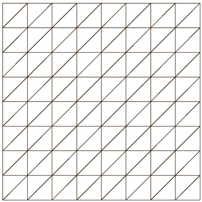
A representative example is shown in Figure 1. The polygonal mesh was generated using [27].

Refer to caption
Refer to caption
Refer to caption
Refer to caption
Figure 1. Sample meshes used in the numerical test corresponding to an 8×88\times 8 subdivision of the domain: triangles, squares, radom quads, and polygons.

We use fixed point iterations analysed in Section 4 to solve the nonlinear system resulting from the VEM discretisation. This is compared below with Newton-Raphson iterations, defined as follows. Given an initial iterate uh0∈Vhu_{h}^{0}\in V_{h}, we construct a sequence uhn+1=uhn+δnu_{h}^{n+1}=u_{h}^{n}+\delta^{n}, n≥0n\geq 0, by solving at each iteration the linearised problem: find δn∈Vh\delta^{n}\in V_{h} such that

(5.1) ah​(uhn,δn,vh)+bh​(uhn,δn,vh)=(Phk−1​f,vh)−ah​(uhn,uhn,vh),∀vh∈Vh.a_{h}(u_{h}^{n};\delta^{n},v_{h})+b_{h}(u_{h}^{n};\delta^{n},v_{h})=({P}_{h}^{k-1}f,v_{h})-a_{h}(u_{h}^{n};u_{h}^{n},v_{h}),\quad\forall v_{h}\in V_{h}.

Here, the extra terms stemming from the linearisation of both the consistency and stability terms in aha_{h} are collected in the global form bh:=∑E∈𝒯hbhEb_{h}:=\sum_{E\in\mathcal{T}_{h}}b_{h}^{E}, with the local form bhEb_{h}^{E}, E∈𝒯hE\in\mathcal{T}_{h}, given by

bhE​(uhn,δn,vh)=\displaystyle b_{h}^{E}(u_{h}^{n};\delta^{n},v_{h})= ∫E𝜿u(Phuhn)Phδk(𝑷h∇uhn)⋅(𝑷h∇vh)d𝒙\displaystyle\int_{E}\bm{\kappa}_{u}({P}_{h}u_{h}^{n}){P}_{h}\delta^{k}(\bm{P}_{h}\,\nabla u_{h}^{n})\cdot(\bm{P}_{h}\,\nabla v_{h})\operatorname{d}\bm{x}
+hEd−2𝜿u(Ph0,Euhn)Ph0,Eδkuhn−Ph​uhn→⋅vh−Ph​vh→.\displaystyle+h_{E}^{d-2}{\bm{\kappa}_{u}({P}_{h}^{0,E}u_{h}^{n})}{P}_{h}^{0,E}\delta^{k}\,\overrightarrow{{u_{h}^{n}}-{P}_{h}u_{h}^{n}}\cdot\overrightarrow{v_{h}-{P}_{h}v_{h}}.

Numerical test. We consider the following test problem from [18]. We solve (1.1) on Ω=[0,1]2\Omega=[0,1]^{2} with 𝜿⁡(u)=1/(1+u)2\bm{\kappa}(u)=1/(1+u)^{2} and the function ff chosen such that the exact solution is u=(x−x2)​(y−y2)u=(x-x^{2})(y-y^{2}). Note that, although the diffusion coefficient is not even bounded on the whole of ℝ{\mathbb{R}}, it is smooth in a neighbourhood of the range of uu. As initial guess for the nonlinear solve we use the constant zero function and the conjugate-gradient method is used to solve the linear system at each iteration. The relative errors for the approximation of uu and its gradient as a function of the mesh size hh are shown in Table 1 for k=1k=1 and a sequence of polygonal meshes, cf. the right-most plot in Figure 1. The numerical results confirm the theoretical rate of convergence. The table also displays the number of fixed point and Newton-Raphson iterations performed until the indicated stopping criteria is reached.

DOF ‖u−Phk​uh‖\|u-{P}_{h}^{k}u_{h}\| EOC ∥∇u−Phk−1∇uh∥\|\nabla u-{P}_{h}^{k-1}\nabla u_{h}\| EOC FP NR
9 1.30E-02 – 9.44E-02 – 6 4
34 3.40E-03 2.018 4.96E-02 0.967 7 4
129 8.16E-04 2.140 2.51E-02 1.022 6 4
510 1.89E-04 2.131 1.25E-02 1.012 6 4
2042 4.49E-05 2.070 6.26E-03 1.001 6 3
8162 1.11E-05 2.011 3.12E-03 1.006 6 3
Table 1. Errors and empirical order of convergence (EOC) on a sequence of polygonal meshes. The Fixed Point and Newton-Raphson iterations needed to reach the tolerance 10−1010^{-10} are reported in the right-most columns.

The convergence history with respect to all meshes in Figure 1 are reported in the loglog plots of Figure 2 showing that the performance is similar in all cases. Note that, as k=1k=1, in the case of the sequence of triangular meshes, the VEM coincides with the standard linear finite element method.

Refer to caption
Refer to caption
Figure 2. Convergence history for k=1k=1 and the sequences of meshes represented in Figure 1.
∥ ∇ u - P h - k 1 ∇ u h ∥ / ∥ ∇ u ∥ / ‖ - u ⁢ P h k u h ‖ ‖ u ‖ ⁢ n D o F ⁢ n D o F

6. Conlusions

With this paper, we show that the Virtual Element Method can be extended to nonlinear problems. In particular, we consider elliptic quasilinear problems with Lipschitz continuous diffusion in two and three dimensions and show that it suffices to evaluate the diffusion coefficient with the component of the VEM solution which is readily accessible. We prove optimal order a priori error estimates under the same mesh assumptions used in the linear setting.

Acknowledgements

This research was initiated during the visit of PC to Leicester funded by the LMS Scheme 2 grant (Project RP201G0158). AC was partially supported by the EPSRC (Grant EP/L022745/1). EHG was supported by a Research Project Grant from The Leverhulme Trust (grant no. RPG 2015-306). All this support is gratefully acknowledged. We also express our gratitude to Martin Nolte (Albert-Ludwigs-Universität Freiburg) and Andreas Dedner (University of Warwick) for supporting the implementation of the VEM within DUNE-FEM.

References

  • [1] Ahmad, B., Alsaedi, A., Brezzi, F., Marini, L. D., and Russo, A. Equivalent projectors for virtual element methods. Computers & Mathematics with Applications 66, 3 (Sept. 2013), 376–391.
  • [2] Antonietti, P. F., Beirão da Veiga, L., Scacchi, S., and Verani, M. A C1C^{1} virtual element method for the Cahn-Hilliard equation with polygonal meshes. SIAM J. Numer. Anal. 54, 1 (2016), 34–56.
  • [3] Antonietti, P. F., Bigoni, N., and Verani, M. Mimetic finite difference approximation of quasilinear elliptic problems. Calcolo 52, 1 (2015), 45–67.
  • [4] Artioli, E., Beirão da Veiga, L., Lovadina, C., and Sacco, E. Arbitrary order 2d virtual elements for polygonal meshes: Part ii, inelastic problem. arXiv:1701.06676.
  • [5] Ayuso de Dios, B., Lipnikov, K., and Manzini, G. The nonconforming virtual element method. ESAIM Math. Model. Numer. Anal. 50, 3 (2016), 879–904.
  • [6] Beirão da Veiga, L., Brezzi, F., Cangiani, A., Manzini, G., Marini, L. D., and Russo, A. Basic principles of virtual element methods. Math. Models Methods Appl. Sci. 23, 1 (2013), 199–214.
  • [7] Beirão da Veiga, L., Lovadina, C., and Russo, A. Stability analysis for the virtual element method. Math. Models Methods Appl. Sci. 27, 13 (2017), 2557–2594.
  • [8] Beirão da Veiga, L., Lovadina, C., and Vacca, G. Virtual elements for the navier-stokes problem on polygonal meshes. arXiv:1703.00437.
  • [9] Beirão da Veiga, L., Brezzi, F., Marini, L. D., and Russo, A. The hitchhiker’s guide to the virtual element method. Math. Models Methods Appl. Sci. 24, 8 (2014), 1541–1573.
  • [10] Beirão da Veiga, L., Brezzi, F., Marini, L. D., and Russo, A. Virtual element methods for general second order elliptic problems on polygonal meshes. Math. Models Methods Appl. Sci. 24 (2016), 729–750.
  • [11] Beirão da Veiga, L., and Manzini, G. A virtual element method with arbitrary regularity. IMA J Numer Anal (published online) (July 2013).
  • [12] Blatt, M., Burchardt, A., Dedner, A., Engwer, C., Fahlke, J., Flemisch, B., Gersbacher, C., Gräser, C., Gruber, F., Grüninger, C., Kempf, D., Klöfkorn, R., Malkmus, T., Müthing, S., Nolte, M., Piatkowski, M., and O., S. The distributed and unified numerics environment, version 2.4. Archive of Numerical Software 4, 100 (2016).
  • [13] Brenner, S. C., Guan, Q., and Sung, L.-Y. Some Estimates for Virtual Element Methods. Comput. Methods Appl. Math. 17, 4 (2017), 553–574.
  • [14] Brenner, S. C., and Scott, L. R. The mathematical theory of finite element methods, third ed., vol. 15 of Texts in Applied Mathematics. Springer, New York, 2008.
  • [15] Cangiani, A., Dedner, A., Diwan, G., and Nolte, M. Virtual element method implementation within dune. In preparation.
  • [16] Cangiani, A., Georgoulis, E. H., Pryer, T., and Sutton, O. J. A posteriori error estimates for the virtual element method. Numer. Math. 137, 4 (2017), 857–893.
  • [17] Cangiani, A., Manzini, G., and Sutton, O. J. Conforming and nonconforming virtual element methods for elliptic problems. IMA J. Numer. Anal. 37, 3 (2017), 1317–1354.
  • [18] Chatzipantelidis, P., Ginting, V., and Lazarov, R. D. A finite volume element method for a non-linear elliptic problem. Numer. Linear Algebra Appl. 12, 5-6 (2005), 515–546.
  • [19] Cockburn, B., Di Pietro, D. A., and Ern, A. Bridging the hybrid high-order and hybridizable discontinuous Galerkin methods. ESAIM Math. Model. Numer. Anal. 50, 3 (2016), 635–650.
  • [20] Di Pietro, D. A., and Droniou, J. A hybrid high-order method for Leray-Lions elliptic equations on general meshes. Math. Comp. 86, 307 (2017), 2159–2191.
  • [21] Douglas, Jr., J., and Dupont, T. A Galerkin method for a nonlinear Dirichlet problem. Math. Comp. 29 (1975), 689–696.
  • [22] Douglas, Jr., J., Dupont, T., and Serrin, J. Uniqueness and comparison theorems for nonlinear elliptic equations in divergence form. Arch. Rational Mech. Anal. 42 (1971), 157–168.
  • [23] Droniou, J., Eymard, R., Gallouët, T., and Herbin, R. A unified approach to mimetic finite difference, hybrid finite volume and mixed finite volume methods. Math. Models Methods Appl. Sci. 20, 2 (2010), 265–295.
  • [24] Dupont, T., and Scott, L. R. Polynomial approximation of functions in Sobolev spaces. Math. Comp. 34, 150 (1980), 441–463.
  • [25] Sutton, O. J. Conforming and nonconforming virtual element methods for elliptic problems. PhD thesis, University of Leicester, 2017.
  • [26] Sutton, O. J. The virtual element method in 50 lines of MATLAB. Numer. Algorithms 75, 4 (2017), 1141–1159.
  • [27] Talischi, C., Paulino, G., Pereira, A., and Menezes, I. Polymesher: a general-purpose mesh generator for polygonal elements written in Matlab. Struct. Multidisc. Optim. 45 (2012), 309–328.