Shortcuts to adiabaticity using flow fields
Abstract
A shortcut to adiabaticity is a recipe for generating adiabatic evolution at an arbitrary pace. Shortcuts have been developed for quantum, classical and (most recently) stochastic dynamics. A shortcut might involve a counterdiabatic Hamiltonian that causes a system to follow the adiabatic evolution at all times, or it might utilize a fast-forward potential, which returns the system to the adiabatic path at the end of the process. We develop a general framework for constructing shortcuts to adiabaticity from flow fields that describe the desired adiabatic evolution. Our approach encompasses quantum, classical and stochastic dynamics, and provides surprisingly compact expressions for both counterdiabatic Hamiltonians and fast-forward potentials. We illustrate our method with numerical simulations of a model system, and we compare our shortcuts with previously obtained results. We also consider the semiclassical connections between our quantum and classical shortcuts. Our method, like the fast-forward approach developed by previous authors, is susceptible to singularities when applied to excited states of quantum systems; we propose a simple, intuitive criterion for determining whether these singularities will arise, for a given excited state.
I Introduction
The acceleration of quantum adiabatic dynamics is a goal shared by a variety of physical applications, including adiabatic quantum computing [1, 2, 3], cold atom transport [4, 5, 6], many-body state engineering [7, 8, 9, 10] and quantum thermodynamics [11, 12, 13]. According to the quantum adiabatic theorem [14, 15], a system evolving under a Hamiltonian remains in an instantaneous energy eigenstate if changes adiabatically (infinitely slowly). If changes rapidly the system develops undesirable excitations, evolving into a superposition of the energy eigenstates. Shortcuts to adiabaticity [16] are protocols that suppress these excitations by means of an auxiliary Hamiltonian , which is added to to achieve the desired evolution. A variety of shortcut protocols have been developed including invariant-based inverse engineering [17, 18], transitionless counterdiabatic driving [19, 20, 21, 22], fast-forward methods [23, 24, 25] and methods based on unitary [26, 27, 28, 29, 30] or gauge [31] transformations. Quantum shortcuts to adiabaticity have been extended to non-Hermitian Hamiltonians [32, 33], open quantum systems [34, 35, 36, 37] and Dirac-dynamics [38, 39, 40]. They have been demonstrated experimentally [41, 42, 43, 44, 45, 46], and their relationship with quantum speed limits has been clarified [47, 48]. Shortcuts to adiabaticity are complimentary to, and are sometimes combined with [49, 50], strategies based on optimal quantum control theory, which impose an optimality criterion to improve the fidelity of evolution [51, 52].
Analogous problems in classical Hamiltonian [22, 53, 29, 54, 55, 56, 57] and stochastic [58, 59, 60, 61, 62] dynamics have recently gained attention. For a classical system in one degree of freedom, evolving under a Hamiltonian , the action is an adiabatic invariant [63]. Classical shortcuts involve constructing an auxiliary Hamiltonian to preserve the action even when changes rapidly. Similarly, the evolution of an overdamped Brownian particle from one thermal equilibrium state to another can be accelerated using an appropriately crafted, time-dependent auxiliary potential. This approach was developed in Ref. [60], where its similarity with quantum and classical shortcuts was noted.
In this paper, we show that a broad class of quantum, classical and stochastic shortcuts to adiabaticity can be described within a simple, unifying framework. In this framework, the construction of the desired auxiliary Hamiltonian proceeds in three steps. First, we identify the adiabatic evolution as the evolution that the system of interest would undergo if the process were performed adiabatically. We then define velocity and acceleration flow fields and that characterize the adiabatic evolution, as illustrated in Figs. 1, 5 and 7 for the quantum, classical and stochastic cases. Finally, from these fields we immediately construct auxiliary terms that provide both “counterdiabatic” (Eqs. 13, 55a, 70) and “fast-forward” (Eqs. 16, 55b) shortcuts.
Our paper is structured as follows. In Sec. II we develop our approach to quantum shortcuts to adiabaticity, in one degree of freedom. After deriving the main results of this section, Eqs. 13 and 16, we compare them with previously obtained shortcuts; we show how they provide insight into the singularities that may arise in the fast-forward approach; we analyze the special case of scale-invariant dynamics; we illustrate our approach with numerical simulations; and we briefly discuss generalizations to three degrees of freedom. In Sec. III we review the results of Ref. [57], where our approach was applied to classical shortcuts to adiabaticity. In Sec. IV we discuss semiclassical connections – or the lack thereof – between the quantum and classical results. In Sec. V we use our approach to construct shortcuts to adiabaticity for an overdamped Brownian particle. We present concluding remarks in Sec. VI.
II Quantum shortcuts
We begin by reviewing two known quantum shortcuts to adiabaticity: transitionless quantum driving and the fast-forward method. The former, due to Demirplak and Rice [19] and Berry [21], involves the counterdiabatic Hamiltonian
| (1) |
where denotes the ’th eigenstate of a Hamiltonian of interest, , and . If a wavefunction evolves under from an initial state , then it remains in the ’th instantaneous eigenstate of at all times, as the term suppresses excitations to other eigenstates [19, 21]. Note that the counterdiabatic term (Eq. 1) does not depend on the choice of . Transitionless quantum driving is derived from basic principles of unitary evolution and is consequently quite general: it applies both to spatially continuous systems such as a particle in a time-dependent potential, and to discrete-state, e.g. spin, systems.
The operator (Eq. 1) is a generator of adiabatic transport [64, 22], in the sense that
| (2) |
aside from an overall phase. Eq. 2 clarifies why adding to produces transitionless driving [22]: for each time step , the evolution operator under is , which first evolves the state to , and then contributes an increment in the dynamical phase, . Here we have taken to be infinitesimal, and have ignored corrections.
The fast-forward approach, due to Masuda and Nakamura [23], pertains to a Hamiltonian of the form
| (3) |
For a given time interval , and a particular quantum number , a “fast-forward” potential is constructed with the following property: if a wavefunction evolves under from the initial state , then it will arrive in the eigenstate (up to an overall phase) at . For intermediate times , the wavefunction is in a superposition of eigenstates of , as illustrated in Fig. 3 of Ref. [23], or Fig. 3 below. The fast-forward potential depends on the chosen quantum number . Moreover, typically (though not always) becomes singular at nodes of the instantaneous eigenstate, that is, where . Hence the applicability of the fast-forward method is generally restricted to the ground state, , although there are exceptions to this statement. We will return to this point later in our discussion.
Both and are auxiliary Hamiltonians that are tailored to achieve the desired acceleration of adiabatic dynamics. We will use the term counterdiabatic () to refer to methods in which the auxiliary term causes the system to follow the adiabatic evolution – at an accelerated pace – for the duration of the process. This is the case with transitionless quantum driving: the wavefunction remains in a given eigenstate of at all times, when evolving under . The term fast-forward () will refer to methods in which the system strays from the adiabatic evolution at intermediate times, but returns to the adiabatic state at the final time , as in the Masuda-Nakamura method. As illustrated by the previous paragraphs, auxiliary terms in the fast-forward approach are local, in the sense that they are explicit functions of and . By contrast, counterdiabatic driving generally requires non-local auxiliary terms, given either by spectral sums (as with Eq. 1) or by expressions involving both coordinates and momenta (see Refs. [22, 29, 55], or Eq. 13 below). Thus, fast-forward auxiliary terms may generically be easier to implement experimentally, than counterdiabatic terms.
In what follows, we bridge the two approaches. We consider a Hamiltonian of interest
| (4) |
in one degree of freedom. We assume that varies with time only during the interval , and that this time-dependence is turned on and off smoothly – specifically, , and are continuous functions of time for all , and for . For a given choice of quantum number , we will define velocity and acceleration flow fields and , that characterize how the eigenstate probability distribution deforms with . From these flow fields we will construct simple expressions for both a counterdiabatic Hamiltonian (Eq. 13), and a local fast-forward potential (Eq. 16).
II.1 Setup and derivation of main results
Let the real-valued wavefunction denote the ’th eigenstate of , with eigenenergy :
| (5) |
For convenience we omit the subscript on and . The adiabatic evolution is identified as follows: 11 1 The dynamical phase is generically accompanied by a geometric phase [75], but the latter vanishes for a kinetic-plus-potential Hamiltonian in one degree of freedom.
| (6) |
When the time-dependence of is quasi-static, is a solution of the Schrödinger equation, [14, 15]. When the time-dependence is arbitrary, obeys
| (7) |
for the counterdiabatic term given by Eq. 1 [19, 21]. Thus the addition of the term causes the system to follow the adiabatic evolution, , when is varied rapidly. In what follows we construct a different counterdiabatic term, given as an explicit function of and (Eq. 13), which accomplishes the same result for a given choice of .

Let us define the integrated probability density function
| (8) |
As is a monotonically increasing function, we can invert it to obtain . We then define a velocity flow field 22 2 The quantity was identified as a “hydrodynamic velocity” in Ref. [25], Eq. (6).
| (9) |
This flow field can be pictured by dividing the area under into strips of equal area, delimited by vertical lines at locations , so that ; see Fig. 1. The locations evolve parametrically with , according to
| (10a) | |||
| Note that Eq. 10a does not reflect the unitary dynamics generated by , but rather the variation of the eigenstate probability density with . We similarly introduce an acceleration flow field, | |||
| (10b) | |||
By Eq. 10a this field satisfies
| (11) |
where the prime and dot denote and , respectively. Both flow fields vanish outside the interval :
| (12) |
as follows from the assumptions spelled out after Eq. 4. We will now use these flow fields to construct counterdiabatic and fast-forward shortcuts, given by Eqs. 13 and 16 below.
We begin by defining the counterdiabatic Hamiltonian,
| (13) |
We claim that the adiabatic wavefunction (Eq. 6) satisfies Eq. 7 for arbitrary time-dependence of , with now given by Eq.13. To show this, we first rearrange Eq. 9 as . Differentiating both sides with respect to leads to the continuity equation , equivalently,
| (14) |
We now use Eqs. 5, 6 and 14 to evaluate the right side of Eq. 7:
| (15) | |||||
which establishes that is a solution of Eq. 7. Thus if a wavefunction evolves under from an initial state , then it remains in the ’th instantaneous eigenstate of during the entire process, just as in the case of transitionless quantum driving [19, 21].
Turning our attention to the fast-forward approach, we construct a potential and a companion function as follows:
| (16) | |||||
| (17) |
By Eq. 11, these functions satisfy
| (18) |
Eqs. 16 and 17 specify and only up to arbitrary functions of time. We use this freedom, along with Eqs. 12 and 18, to impose the conditions
| (19) |
and
| (20) |
Eq. 12 further implies that
| (21) |
where are constants (i.e. independent of ).
We now show that the ansatz
| (22) |
is a solution of the Schrödinger equation
| (23) |
Evaluating the right side with the help of Eqs. 5, 14, 17 and 20, we obtain
| (24) | |||||
which is the desired result. By Eq. 21, the wave function begins in the ’th energy eigenstate at and ends in the ’th energy eigenstate at , which establishes that produces fast-forward evolution.
Note that we introduced the function (Eq. 17) only to facilitate the derivation of our fast-forward approach. This function need not be evaluated if one simply wishes to construct the potential . That potential can be determined directly from the acceleration field , by Eq. 16.
Also, we imposed Eq. 19 so as to obtain an auxiliary potential that is turned on at and off at , but this condition is not necessary. Any satisfying Eq. 16 will provide a shortcut that transports the ’th eigenstate of to the ’th eigenstate of . The addition of an arbitrary function to affects only the overall phase of the evolving wavefunction.
II.2 Comparison with previous results
Eqs. 13 and 16 are recipes for constructing shortcuts directly from the flow fields and . Let us compare these results with previously published counterdiabatic and fast-forward shortcuts.
Our result for (Eq. 13) is given explicitly in terms of the operators and . This appealing feature comes with a cost: in general, a different counterdiabatic term is required for each eigenstate , since depends on the choice of . By contrast the Demirplak-Rice-Berry [19, 21] counterdiabatic term (Eq. 1) is independent of , as noted earlier. We conclude that Eqs. 1 and 13 are not equivalent, although the two counterdiabatic terms produce the same effect when they act on the chosen adiabatic eigenstate:
| (25) |
Using the identity , which holds for given by Eq. 4, we rewrite the equality in Eq. 25 as follows:
| (26) |
In other words, the operator acts as the generator of adiabatic transport (see Eq. 2) for the state that was used to construct :
| (27) |
for infinitesimal .
Substituting Eq. 17 into Eq. 14 yields
| (28) |
Eqs. 20 and 28 are essentially equivalent to Eqs. 5 and 6 of Torrontegui et al [24], to Eqs. 17 and 15 of Takahashi [30], and to Eqs. 4 and 3 of Martínez-Garaot et al [25]. In Refs. [24, 30, 25] these equations were used to provide streamlined derivations of the fast-forward approach pioneered by Masuda and Nakamura [23]. (Our Eq. 28 is also equivalent to Eq. 2.18 of Ref. [23], and our Eq. 17 appears as Eq. 5 in Ref. [25].) Thus our fast-forward potential is equivalent to that derived by previous authors [23, 24, 30, 25].
The observation that the quantum counterdiabatic and fast forward approaches are closely related is not surprising, as previous authors have argued that can be constructed from by appropriate unitary [26, 27, 28, 29, 30] or gauge [31] transformations. The novelty of our approach is that we obtain both and directly from the velocity and acceleration fields that describe the time-dependence of (Fig. 1). Our results are given by compact, intuitive expressions (Eqs. 13, 16). This approach highlights the connection between counterdiabatic and fast-forward shortcuts, and – as we shall see – it provides insight into the divergences that often plague the fast-forward method when it is applied to excited states. Moreover, the construction of and from and is mirrored in classical shortcuts to adiabaticity, as will be discussed in Sec. III.
Finally, we note that Eq. 20 is a Hamilton-Jacobi equation for the Hamiltonian . Okuyama and Takahashi [56] have recently used the Hamilton-Jacobi formalism to explore the correspondence between quantum and classical shortcuts to adiabaticity. It would be interesting to explore the relationship between their approach and ours.
II.3 Divergences and a “no-flux” criterion
By Eq. 9, generically diverges at nodes of the wavefunction, where vanishes; this in turn leads to divergences in , and in and . These observations suggest that our method is in general restricted to ground state wavefunctions (), which have no nodes.
While nodes in typically spoil the applicability of our method, this need not always be the case: the numerator and denominator in Eq. 9 might vanish simultaneously in a way that prevents the ratio from blowing up at a node. Here we propose a simple criterion for determining whether our approach (and by extension the fast-forward approach [23, 24, 30, 25]) is applicable when an eigenstate has one or more nodes.
Let denote the location, and the velocity, of the ’th node of . We assume , as will generally be the case when the potential is well-behaved. As varies parametrically, the flux of probability across this node, from the region to the region , is given by
| (29) |
using Eqs. 8 and 9. This result has the familiar interpretation of “flux equals velocity times density”, in the node’s co-moving frame of reference. Eq. 29 implies that if does not blow up at a given node, then the probability flux across that node must be zero. This suggests a simple criterion: if the time-dependence of is such that there is no flux of probability across any node, i.e. if for all , then the velocity field will not diverge at the nodes and our method will remain valid and applicable 33 3 In fact, if then , although we will not make use of this result here. . Generalizing the term “nodes” to include the boundaries at , the no-flux criterion can alternatively be stated as follows: if the probability between all pairs of adjacent nodes remains independent of [i.e. if for all ], then will be free of divergences and will be well-behaved.
This “no-flux” criterion is not generically satisfied for given by Eq. 4. However, in Sec. II.4 we consider a particular class of time-dependent Hamiltonians for which this criterion is satisfied for every eigenstate, due to scale-invariance (Eq. 30). In agreement with the arguments presented above, our method provides non-singular counterdiabatic and fast-forward shortcuts for all energy eigenstates, for this class of Hamiltonians. In Sec. II.5 we present the results of numerical simulations for a non-scale-invariant Hamiltonian, for which the no-flux criterion is satisfied for the first excited state; again, our method successfully provides a non-singular shortcut for this situation.
Divergences associated with eigenstate nodes are problematic not only for our approach, but also for those of Refs. [23, 24, 30, 25], since all these approaches lead to equivalent expressions for . This problem has not received much attention in the literature, although Martínez-Garaot et al [25] consider it in a slightly different context. In Sec. III.D of their paper, they develop a fast-forward strategy to drive a wavefunction from a ground state to a first excited state . In their approach the fast-forward potential becomes singular due to the node in , but they demonstrate that ad hoc truncation of the singularity produces a well-behaved potential that achieves near-perfect fidelity. It would be interesting to test whether such truncation is also useful in the context of our method, when the no-flux criterion is not satisfied.
II.4 Scale-invariant dynamics
In the special case of scale-invariant driving, undergoes expansions, contractions and translations. As shown in Ref. [29] (and anticipated in Refs. [65, 66, 67, 68, 27, 22, 53]), simple expressions for counterdiabatic and fast-forward shortcuts can be obtained when a system is driven in a scale-invariant manner. In this section we show that these shortcuts are obtained naturally within our framework.
The Hamiltonian for scale-invariant driving takes the form [29]
| (30) |
where and are parameters that describe expansions/contractions, and translations, respectively. If we let denote the ’th eigenstate of , then the ’th eigenstate for a general choice of is given by [29]
| (31) |
This scaling result immediately reveals how the “picket fence” of lines depicted in Fig. 1 behaves when and are varied with time. Variations in result in translations of the entire picket fence, and variations in cause the picket fence to expand or contract linearly. These considerations give us
| (32) |
and therefore (by Eq. 11)
| (33) |
Eq. 32 also follows from Eq. 9, , since and (making use of Eq. 31)
| (34) | |||||
Combining Eqs. 32 and 33 with Eqs. 13 and 16, we obtain
| (35a) | |||||
| (35b) | |||||
in agreement with Eqs. 9 and 30 of Ref. [29]. Thus the shortcuts obtained previously for scale-invariant driving emerge naturally within our framework, from the flow fields and (Eqs. 32, 33).
We end this section by highlighting two exceptional features of scale-invariant Hamiltonians, both of which are due to the fact that all of the eigenstates of satisfy the same scaling property, Eq. 31. First, although denotes a specific energy eigenstate in the above calculations, the resulting flow fields and shortcuts (Eq. 35) are independent of the choice of . This suggests that for scale-invariant driving, in contrast with the general situation discussed in Sec. II.2. Indeed, it has been shown elsewhere that Eq. 35a – which we derived from Eq. 13 – follows directly from Eq. 1 [29]. Secondly, the shortcuts given by Eq. 35 do not suffer from divergences at the nodes of excited energy eigenstates. This is easy to understand in terms of the no-flux criterion of Sec. II.3: because variations in merely cause the eigenstate to expand or contract linearly, and variations in induce simple translations of , the probability between adjacent nodes of the wavefunction is independent of .
II.5 Numerical illustration of fast-forward driving
The parameter-dependent potential
| (36) |
belongs to a class of potentials studied by Razavy [69], for which convenient analytical expressions for low-lying eigenstates can be obtained. Here and below, we have set the quantities , and (appearing in Ref. [69]) to unity, so as to work with an effectively dimensionless Hamiltonian. As illustrated in Fig. 2, changes from a broad double well to a narrow single well as is increased from 0.1 to 6.0.
Now consider
| (37) |
where varies monotonically from to over the interval , according to
| (38) |
and remains constant outside this interval. Note that and , hence satisfies the continuity conditions described after Eq. 4.
The wavefunction for the first excited state of is given by [69]
| (39) |
where is set by normalization. The corresponding eigenenergy is . Although this eigenstate has a node at the origin, the no-flux criterion of Sec. II.3 is satisfied by the anti-symmetry of the wavefunction: , hence for all . Thus we expect our approach to apply despite the presence of the node.

Using the above expressions and setting , we numerically computed the function (Eq. 8), from which we constructed the flow fields and and the fast-forward potential (Eq. 16). As increases from to , becomes increasingly narrow (Fig. 2), as does the eigenstate ; this is reflected in the fields and , which describe the flow of probability toward the origin. initially develops into a potential well that resembles a parabola (though it is not precisely quadratic) – this brings about the acceleration of probability flow toward the origin. At later times during the process resembles an inverted parabola, which effectively decelerates this flow.
We performed two numerical simulations of evolution under the time-dependent Schrödinger equation
| (40) |
using in the first simulation and in the second; we will use the notation and to distinguish between the two simulations. In both cases the wavefunction was initialized in the state . The time evolution was performed using the split-time propagation scheme [70, 71], which involves the repeated application of the fast Fourier transform to toggle between the position and momentum representations.
Fig. 3 shows snapshots of (solid lines) and (dashed lines) for both simulations. Note that in the adiabatic limit (Eq. 6) – this is our motivation for plotting rather than , though in the following paragraphs we largely will stop writing the factor , for convenience.
The upper panel of Fig. 3 shows the evolution of . Due to the nonadiabatic time-dependence of , the wavefunction “lags” behind the instantaneous eigenstate . This is particularly evident in Fig. 3(b), where the probability associated with has shifted substantially toward the origin, while remains somewhat behind. This lag leads to shock waves, which are nascent in Fig. 3(b). These shocks propagate inward, and ends in a superposition of excited states [Fig. 3(c)].
The lower panel shows the evolution of . Here the wavefunction develops excitations at short times [Fig. 3(d)], in response to large forces generated by . These forces eliminate the lag that is observed in the upper panel, by “squeezing” the wavefunction and causing probability to accelerate toward the origin. At later times this flow is decelerated – again, due to – and the excitations subside [Fig. 3(e)]. The wavefunction gently arrives at the desired energy eigenstate at the final time [Fig. 3(f)].
In the present context Eq. 22 can be written as
| (41) |
which implies that the probability densities at all times, despite the excitations that develop in . We have verified this result in our simulations (data not shown). Eq. 41 further implies that , which is illustrated in Fig. 3(d), where the dashed line is manifestly the envelope of the solid line.
Finally, for both simulations we computed the fidelity , that is the degree of overlap between the evolving wavefunction and the energy eigenstate. Fig. 4 shows the results. In the absence of the auxiliary term, the fidelity decays monotonically to . When is included in the Hamiltonian, the fidelity at first drops rapidly to nearly zero – due to the excitations that develop in – but then it claws its way back to unity, illustrating the effectiveness of the fast-forward potential obtained from the acceleration flow field .
II.6 Extension to three degrees of freedom
Although the focus in this paper is on systems with one degree of freedom, here we briefly discuss how the results of Sec. II.1 might be extended to three dimensions. We will use boldface to denote vector quantities.
For a given choice of quantum number , let and denote the ’th eigenstate and eigenenergy, respectively, of the Hamiltonian given by Eq. 3. Let us define a vector field by the equation
| (42) |
which describes how the eigenstate probability density varies parametrically with . We assume that and its first two time derivatives vanish outside the interval (as in the one-dimensional case), therefore can be constructed to vanish outside this interval as well: for . 44 4 Eq. 42 defines only up to gauge-like transformations of the form , where is an arbitrary, well-behaved vector field. Hence we have some freedom in constructing . This freedom was not present in Sec. II.1, where the was defined using the construction shown in Fig. 1, rather than from the continuity equation.
Since Eq. 42 is a continuity equation, it can be interpreted as describing an ensemble of independent trajectories, each evolving according to . The acceleration of these trajectories is described by a field whose ’th component satisfies
| (43) |
We now define a counterdiabatic Hamiltonian
| (44) |
Using (which follows from Eq. 42), it is readily verified that the wavefunction
| (45) |
is a solution of the Schrödinger equation .
Now let us suppose that the field can be chosen to be curl-free:
| (46) |
We can then introduce a function that satisfies
| (47) |
which allows us to rewrite Eq. 43 as
| (48) |
We have used both Eqs. 46 and 47 in going from Eq. 43 to Eq. 48. If we now define by the equation
| (49) |
then Eq. 48 implies (compare with Eq. 16). It is now a matter of algebra to verify that obeys the Schrödinger equation . Since is a constant outside the interval , we see that the addition of the fast-forward potential causes the chosen eigenstate of the initial Hamiltonian to evolve to the corresponding eigenstate of the final Hamiltonian.
As in the one-dimensional case, divergences in may arise whenever , potentially causing the method to break down for excited eigenstates. This issue deserves further exploration.
III Classical shortcuts
In this section we briefly review the procedure developed in Ref. [57] for obtaining counterdiabatic and fast-forward shortcuts for a classical Hamiltonian of interest
| (50) |
As in Sec. II, varies with time only during the interval , and this time-dependence is turned on and off smoothly, as per comments following Eq. 4. Let denote the classical action, where the integral is taken around an energy shell, that is a level curve of , containing the point . The action is equal to the volume of phase space enclosed by the energy shell, and it is an adiabatic invariant [63]: in the limit of adiabatic (quasi-static) driving, the value of remains constant along a trajectory evolving under . Thus, the adiabatic evolution is identified in the classical case with the preservation of the action along the trajectory.
If is the constant value of the action along a trajectory evolving under adiabatic conditions, then the value of the Hamiltonian along the trajectory, , is determined by the condition
| (51) |
The notation indicates that the line integral is carried out around the energy shell . We will refer to this shell as the adiabatic energy shell, and to as the adiabatic energy. The action value and the adiabatic energy are classical analogues of the quantum number and eigenenergy .
We now assume that varies at an arbitrary – i.e. non-adiabatic – rate, but we continue to use the term adiabatic energy to refer to defined by Eq. 51, for chosen value of action, . For a trajectory with initial action , we wish to construct a counterdiabatic Hamiltonian and a fast-forward potential such that: (1) if the trajectory evolves under , it remains on the adiabatic energy shell at all times, that is, ; and (2) if the trajectory evolves under , it returns to the adiabatic energy shell at the final time: . Here and below, denotes the value of the action function along the trajectory.
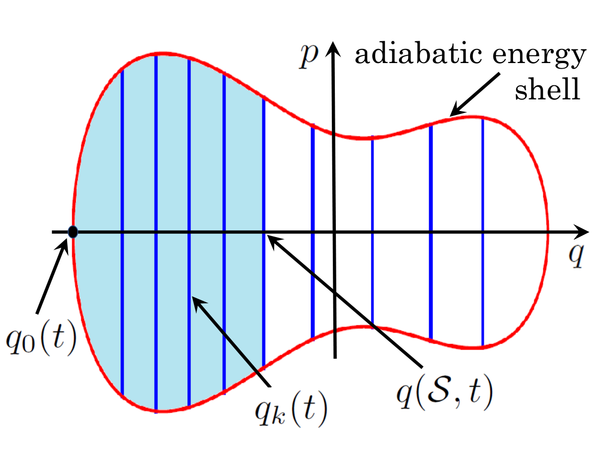
To construct these shortcuts for a given choice of , let
| (52) |
specify the upper branch of the adiabatic energy shell, and let
| (53) |
denote the volume of phase space enclosed by the adiabatic energy shell between the left turning point and a point . The function is monotonically increasing and therefore can be inverted to obtain , which in turn is used to define flow fields
| (54a) | |||||
| (54b) | |||||
These flow fields are pictured by dividing the adiabatic energy shell into strips enclosing equal phase space volume, delimited by lines drawn at locations ; see Fig. 5. The fields and describe the motion of these lines as the parameter is varied: and .
Using these flow fields we now define a counterdiabatic Hamiltonian
| (55a) | |||
| and a fast-forward potential that satisfies | |||
| (55b) | |||
both of which vanish for . As shown in Ref. [57], if a trajectory evolves under the Hamiltonian , then the action is preserved along the entire trajectory: for all . If the trajectory instead evolves under , then the initial and final action values are equal, , though at intermediate times. In both cases the action is defined with respect to the Hamiltonian , and the construction of and depends on the choice of action .
Figure 6 illustrates evolution under the fast-forward Hamiltonian . The trajectories begin on the adiabatic energy shell, they evolve away from it at intermediate times, and return to it at the final time.
IV Comparison of quantum and classical shortcuts
As proposed in Ref. [22] and illustrated in Ref. [55], a classical counterdiabatic Hamiltonian emerges when the right side of Eq. 1 is evaluated in the semiclassical limit. Similarly, it is natural to speculate that the classical shortcuts of Sec. III are the semiclassical limit of the quantum shortcuts of Sec. II. In that case the close similarity between Eqs. 55a, 55b and Eqs. 13, 16 would simply reflect the Correspondence Principle. In the following paragraph we address this issue by asking whether the flow fields and defined in Sec. III emerge from those of Sec. II in the semiclassical limit (). We will temporarily use the superscript (for “quantum”) to denote certain quantities defined in Sec. II, to denote their semiclassical limits, and to denote quantities defined in Sec. III.
When we consider the semiclassical limit of the field (Eq.9), we immediately run into a difficulty: the divergences discussed in Sec. II.3 proliferate in this limit, as the number of nodes of becomes large. This proliferation of divergences (nodes) arises from the rapid spatial oscillations of high-lying eigenstates . To obtain a non-singular velocity field, we replace the oscillatory probability density (used to construct ) by a locally averaged counterpart, , that smooths over these oscillations. The semiclassical limit of is the microcanonical probability distribution, projected from phase space onto the coordinate axis [15]:
| (56) |
with given by Eq. 52. Using in place of in Eq. 8 we obtain
| (57) |
We use this function to define , which is free of divergences and can be viewed as the semiclassical limit of (Eq. 9). Comparing with the field defined by Eq. 54a, we see that while one is constructed from the integrated microcanonical distribution , the other is constructed in terms of the phase space enclosed by the energy shell, . Therefore, in general, the two fields differ: . We conclude that Eq. 55a should not be viewed as the semiclassical limit of Eq. 13. Similar comments apply to the acceleration field .
We summarize the situation as follows: while the flow fields and are defined similarly in the quantum and classical cases (compare Figs. 1 and 5), and while the construction of counterdiabatic and fast-forward terms from the flow fields is essentially identical in the two cases, the Correspondence Principle does not provide an adequate explanation for this striking similarity. We also note that scale-invariant driving (Eq. 30) provides an exception to this general conclusion: in that case the quantum and classical flow fields are in fact identical [29, 57].
As a final item of semiclassical comparison, let us consider trajectories evolving under the classical Hamiltonian , with initial conditions sampled from the adiabatic energy shell (Fig. 6). It was shown in Ref. [57] that the function
| (58) |
remains constant along these trajectories: for all . This is illustrated in Fig. 6, where the thick red curve is obtained by “boosting” the thin black curve – the adiabatic energy shell – by an amount along the momentum direction. Now consider the fast-forward wavefunction (Eq. 22) evolving under Let us approximate the eigenstate by the WKB form [15]
| (59) |
where . The terms on the right side of Eq. 59 represent a right-moving wave train and a left-moving wave train, with local momenta corresponding to the upper and lower branches of the adiabatic energy shell (Fig. 5). Then for the fast-forward wavefunction we get
| (60) |
since (Eq. 17). The terms in Eq. 60 are wave trains with local momenta . Thus the fast-forward wavefunction is represented, in the WKB sense, by a “boosted” adiabatic energy shell similar to the one shown as a thick red curve in Fig. 6. Although this interpretation provides a neat correspondence between the quantum and classical fast-forward methods, it should not be taken too literally, since the fast-forward method of Sec. II generally applies only to the ground state (as discussed earlier), where the WKB approximation (Eq. 59) is not generally accurate.
V Shortcuts for stochastic systems

Finally, let us consider an overdamped Brownian particle in a time-dependent potential , which varies smoothly for but is fixed outside this interval. The particle is in contact with a thermal reservoir at temperature . The interactions with the degrees of freedom of the reservoir give rise to the random and dissipative forces that characterize Brownian dynamics.
We will work in the ensemble picture, in which the dynamics are described by a probability density function that evolves according to the Fokker-Planck equation
| (61) |
The friction and diffusion coefficients, and , obey the Einstein-Smoluchowski relation, , where is the Boltzmann constant. The equilibrium distribution associated with the potential is given by
| (62) |
It is straightforward to verify the identity
| (63) |
which confirms that the equilibrium distribution is a stationary solution of the dynamics, when the potential does not vary with time. When changes quasi-statically, then the slowly varying is a solution of Eq. 61 (both sides tend toward zero in that limit), as expected for a reversible process. Therefore, the adiabatic evolution is identified by the ensemble evolving through the continuous sequence of equilibrium states . 55 5 Here we use the term adiabatic consistently with its usage in the rest of the paper, namely to denote a slow process. This differs from its usage in thermodynamics, where an adiabatic process is one in which heat is not absorbed or released by a system. The dual meaning of this term is unfortunate.
We now consider the case in which the potential is varied at an arbitrary rate. To this potential we will add a counterdiabatic term , so that the system evolves under
| (64) | |||||
We wish to design so as to achieve adiabatic evolution, i.e. so that (Eq. 62) is an exact solution of Eq. 64. This problem has recently been studied by Li, Quan and Tu [62], who use a somewhat different derivation to arrive at the same solution as the one we obtain below (Eq. 70).
We define an integrated distribution
| (65) |
similar to (Eq. 8). Inverting this function to obtain (see Fig. 7), we construct a velocity flow field
| (66) |
Rearranging this result as and differentiating with respect to produces the continuity equation
| (67) |
Since we wish to be a solution of Eq. 64, we use Eqs. 63 and 67 to rewrite that equation as follows:
| (68) |
Integrating both sides gives
| (69) |
Here, is an arbitrary function of time that we set to zero, for convenience, arriving at the result
| (70) |
Eq. 70 defines up to an additive function of time that has no influence on the dynamics, and which can be adjusted so that for . The potential has the desired counterdiabatic property: when the system evolves in the time-dependent potential , it remains in equilibrium (with respect to over the entire duration of the process. Our potential is equivalent to the auxiliary potential obtained by Li et al [62], as can be seen by differentiating both sides of Eq. 12 of Ref. [62] with respect to .
Eq. 70 has elements in common with both the counterdiabatic and fast-forward shortcuts of previous sections. It is counterdiabatic in that the system follows the adiabatic evolution (it remains in the state ) at all times. Moreover, is given in terms of the velocity field (compare Eqs. 13, 55a, and 70), rather than the acceleration field . However, just as with the fast-forward shortcuts described earlier, is local, i.e. it is a time-dependent potential (compare Eqs. 16, 55b, and 70). Also, as in Secs. II and III, Eq. 70 defines the auxiliary potential only up to an arbitrary function of time that does not affect the dynamics.
When our Brownian particle evolves under alone, the state of the ensemble, , lags behind the instantaneous equilibrium state, , as illustrated in Ref. [72], Figure 1. The addition of the counterdiabatic potential eliminates this lag. Lagging distributions are relevant for numerical free-energy estimation methods, where the lag gives rise to poor convergence of the free-energy estimate. Vaikuntanathan and Jarzynski [58] have developed a method in which this lag is reduced or eliminated by the addition of an artificial flow field to the dynamics, although in Ref. [58] this flow field was not related to an auxiliary potential . Comparing Eq. 67 above with Eq. 15 of Ref. [58], we see that our field is equivalent to the perfect flow field () that “escorts” the system faithfully along the equilibrium path.
As a simple example, which makes a connection to the engineered swift equilibration approach recently developed and validated experimentally by Martínez et al [60], we consider a time-dependent harmonic potential,
| (71) |
The instantaneous equilibrium distribution is
| (72) |
Eq. 65 then gives
| (73) |
where is the Gaussian error function. In turn, Eq. 66 yields , and from there we use Eq. 70 to obtain
| (74) |
Therefore, under a harmonic trap of stiffness
| (75) |
the ensemble remains in the equilibrium state (Eq. 72) at all times.
Rearranging Eq. 75 and using , we get
| (76) |
This result is identical to Eq. 6 of Martínez et al [60], where the goal was to bring the system rapidly to the final equilibrium state, without concern for the intermediate states visited along the way. Our approach achieves the same result by guiding the system along the equilibrium path during the entire process. Eq. 76 was also obtained by Schmiedl and Seifert, in the contexts of optimal finite-time control [73] and stochastic heat engines [74].
While our analysis has been restricted to overdamped Brownian motion, Le Cununder and colleagues [61] have recently used a micromechanical cantilever to implement engineered swift equilibration for an underdamped harmonic oscillator. For underdamped motion in a general one-dimensional, time-dependent potential, Li, Quan and Tu [62] have proposed a momentum-dependent counterdiabatic term that achieves the desired adiabatic evolution. It remains to be seen whether this progress will lead to expressions for a momentum-independent counterdiabatic potential that extends the fast-forward method to underdamped Brownian dynamics beyond the harmonic regime.
VI Conclusions
We have developed a framework for constructing counterdiabatic and fast-forward shortcuts for quantum, classical and stochastic systems. This framework is organized around velocity and acceleration flow fields and , which describe the time-dependence of the desired adiabatic evolution. Once the flow fields have been determined, the shortcuts are given by simple expressions involving these fields (Eqs. 13, 16, 55a, 55b, 70).
The flow fields themselves are defined similarly, but not identically, in the three cases – quantum, classical, and stochastic. In each case these fields can be pictured in terms of the evolution of an appropriately defined “picket fence” of lines (Figs. 1, 5, 7) that glide around as time is varied parametrically. Formally, the fields and are constructed from integrated functions, , and , that define the picket fence.
Since both the classical and quantum cases involve an isolated system evolving under a time-dependent Hamiltonian, it might be expected that they are related by the Correspondence Principle. However, we argued in Sec. IV that in the semiclassical limit, the integrated function used in the quantum case, , does not converge to the one used in the classical case, , even after appropriate local averaging to smooth over divergences. In this sense the quantum shortcuts of Sec. II do not converge to the classical ones of Sec. III as . Hence the Correspondence Principle does not provide a satisfactory understanding of the conspicuous similarity between the expressions for and (Eqs. 13, 16), and those for and (Eqs. 55a, 55b).
As noted in Sec. II.3, the nodes of excited energy eigenstates generically pose a problem for our method, as they do for the fast-forward approach in general. The divergences in that result from these nodes can be understood intuitively by considering Eq. 29, which gives the probability flux across the ’th node: . The two factors on the right represent the flow velocity relative to the motion of the node, , and the local density, . If we momentarily imagine that is very small but non-zero at , then we see that must be very large in order to “push through” a fixed probability flux – an apt analogy is water flowing through a pipe that becomes narrow at a certain point. Thus diverges as : an infinite velocity is required to achieve a finite flux, at vanishing probability density.
When the time-dependence of is such that there is no flux of probability across nodes, i.e. when the probability between neighboring nodes remains constant even as the eigenstate deforms, then the flow fields and are non-singular and we expect our method (and more generally the fast-forward approach [23]) to work well. This no-flux criterion is satisfied for scale-invariant driving, as well as for the model system studied numerically in Sec. II.5. In the latter case the criterion is satisfied because the potential (Eq. 36) is symmetric about the origin. It would be useful to identify a more generic (i.e. non-symmetric) potential and eigenstate for which the no-flux criterion is satisfied, and to test whether our method continues to work in that situation. This would provide a more stringent test of the no-flux criterion than the one studied in Sec. II.5.
Our framework connects the counterdiabatic and fast-forward approaches. In the quantum case, the fields and provide two mathematical descriptions the same flow of probability. The former defines the counterdiabatic Hamiltonian , while the latter (together with the mass, ) determines the fast-forward potential . It is remarkable that no other input is required to construct these shortcuts. For the moment we lack a deeper or intuitive understanding of why this should be the case. Analogous comments apply to the classical shortcuts of Sec. III.
Finally, an open problem remains the development of fast-forward shortcuts for excited states of quantum systems, when the no-flux criterion is not satisfied. We are currently investigating whether the insights provided by our approach, based on flow fields, might yield either exact or approximate solutions to this problem. Another question worth exploring is whether our flow-fields method can be extended to obtain shortcuts for open quantum systems [34, 35, 36, 37].
Acknowledgments
We gratefully acknowledge financial support from the U.S. National Science Foundation under grant DMR-1506969 (CJ), and the U.S. Army Research Office under contract number W911NF-13-1-0390 (AP), and stimulating discussions with Alexander Boyd, Sebastian Deffner, Adolfo del Campo, Anatoli Polkovnikov and Yiğit Subaşı.
References
- [1] M. S. Sarandy, E. I. Duzzioni, and R. M. Serra, Phys. Lett. A 375, 3343 (2011).
- [2] A. C. Santos and M. S. Sarandy, Nat. Sci. Rep. 5, 15775 (2015).
- [3] M. A. Nielsen and I. L. Chuang, Quantum Computation and Quantum Information (Cambridge University Press, Cambridge, UK, 2000).
- [4] X. Chen, A. Ruschhaupt, S. Schmidt, A. del Campo, D. Guéry-Odelin, and J. G. Muga, Phys. Rev. Lett. 104, 063002 (2010).
- [5] E. Torrontegui, S. Ibáñez, X. Chen, A. Ruschhaupt, D. Guéry-Odelin, and J. G. Muga, Phys. Rev. A 83, 013415 (2011).
- [6] R. Bowler, J. Gaebler, Y. Lin, T. R. Tan, D. Hanneke, J. D. Jost, J. P. Home, D. Leibfried, and D. J. Wineland, Phys. Rev. Lett. 109, 080502 (2012).
- [7] A. del Campo, Phys. Rev. A 84, 031606(R) (2011).
- [8] A. del Campo, M. M. Rams, and W. H. Zurek, Phys. Rev. Lett. 109, 115703 (2012).
- [9] S. Masuda, K. Nakamura, and A. del Campo, Phys. Rev. Lett. 113, 063003 (2014).
- [10] V. Mukherjee, S. Montangero, and R. Fazio, Phys. Rev. A 93, 062108 (2016).
- [11] P. Salamon, K. H. Hoffmann, Y. Rezek, and R. Kosloff, Phys. Chem. Chem. Phys. 11, 1027 (2009).
- [12] Y. Rezek, P. Salamon, K. H. Hoffman, and R. Kosloff, Euro. Phys. Lett. 85, 30008 (2009).
- [13] P. Skrzypczyk, J. A. Short, and S. Popescu, Nat. Comm. 5, 4185 (2014).
- [14] M. Born and V. A. Fock, Zeitschrift für Physik A 51, 165 (1928).
- [15] D. J. Griffiths, Introduction to Quantum Mechanics (Pearson Prentice Hall, 2004), 2nd ed.
- [16] E. Torrontegui, S. Ibáñez, S. Martínez-Garaot, M. Modugno, A. del Campo, D. Guéry-Odelin, A. Ruschhaupt, X. Chen, and J. G. Muga, Adv. At. Mol. Opt. Phys. 62, 117 (2013).
- [17] X. Chen, E. Torrontegui, and J. G. Muga, Phys. Rev. A 83, 062116 (2011a).
- [18] E. Torrontegui, S. Martínez-Garaot, and J. G. Muga, Phys. Rev. A 89, 043408 (2014).
- [19] M. Demirplak and S. A. Rice, J. Phys. Chem. A 107, 9937 (2003).
- [20] M. Demirplak and S. A. Rice, J. Phys. Chem. B 109, 6838 (2005).
- [21] M. V. Berry, J. Phys. A: Math. Theor. 42, 365303 (2009).
- [22] C. Jarzynski, Phys. Rev. A 88, 040101(R) (2013).
- [23] S. Masuda and K. Nakamura, Proc. R. Soc. A 466, 1135 (2010).
- [24] E. Torrontegui, S. Martínez-Garaot, A. Ruschhaupt, and J. G. Muga, Phys. Rev. A 86, 013601 (2012).
- [25] S. Martínez-Garaot, M. Palmero, J. G. Muga, and D. Guéry-Odelin, Phys. Rev. A 94, 063418 (2016).
- [26] S. Ibáñez, X. Chen, E. Torrontegui, J. G. Muga, and A. Ruschhaupt, Phys. Rev. Lett. 109, 100403 (2012).
- [27] A. del Campo, Phys. Rev. Lett. 111, 100502 (2013).
- [28] S. Martínez-Garaot, E. Torrontegui, X. Chen, and J. G. Muga, Phys. Rev. A 89, 053408 (2014).
- [29] S. Deffner, C. Jarzynski, and A. del Campo, Phys. Rev. X 4, 021013 (2014).
- [30] K. Takahashi, Phys. Rev. A 91, 042115 (2015).
- [31] D. Sels and A. Polkovnikov, Proc. Natl. Acad. Sci. USA 114, 3909 (2017).
- [32] S. Ibáñez, S. Martínez-Garaot, X. Chen, E. Torrontegui, and J. G. Muga, Phys. Rev. A 84, 023415 (2011).
- [33] B. T. Torosov, G. D. Valle, and S. Longhi, Phys. Rev. A 87, 052502 (2013).
- [34] J. Jing, L.-A. Wu, M. S. Sarandy, and J. G. Muga, Phys. Rev. A 88, 053422 (2013).
- [35] G. Vacanti, R. Fazio, S. Montangero, G. M. Palma, M. Paternostro, and V. Vedral, New J. Phys. 16, 053017 (2014).
- [36] J. Song, Z. Zhang, Y. Xia, X. Sun, and Y. Jiang, Opt. Exp. 24, 21674 (2016).
- [37] J. Jing, M. S. Sarandy, D. A. Lidar, D.-W. Luo, and L.-A. Wu, Phys. Rev. A 94, 042131 (2016).
- [38] S. Deffner, New Journal of Physics 18, 012001 (2016).
- [39] J. G. Muga, M. A. Simón, and A. Tobalina, New. J. Phys. 18, 021005 (2016).
- [40] X. Song, F. Deng, L. Lamata, and J. G. Muga, Phys. Rev. A 95, 022332 (2017).
- [41] J.-F. Schaff, X.-L. Song, P. Vignolo, and G. Labeyrie, Phys. Rev. A 82, 033430 (2010).
- [42] J.-F. Schaff, X.-L. Song, P. Capuzzi, P. Vignolo, and G. Labeyrie, Europhys. Lett. 93, 23001 (2011).
- [43] M. G. Bason, M. Viteau, N. Malossi, P. Huillery, E. Arimondo, D. Ciampini, R. Fazio, V. Giovannetti, R. Mannella, and O. Morsch, Nature Physics 8, 147 (2011).
- [44] A. Walther, F. Ziesel, T. Ruster, S. T. Dawkins, K. Ott, M. Hettrich, K. Singer, F. Schmidt-Kaler, and U. Poschinger, Phys. Rev. Lett. 109, 080501 (2012).
- [45] J. Zhang, J. Hyun Shim, I. Niemeyer, T. Taniguchi, T. Teraji, H. Abe, S. Onoda, T. Yamamoto, T. Ohshima, J. Isoya, et al., Phys. Rev. Lett. 110, 240501 (2013).
- [46] S. An, D. Lv, A. del Campo, and K. Kim, Nat. Comm. 7, 12999 (2016).
- [47] S. Deffner and S. Campbell, Phys. Rev. Lett. 118, 100601 (2017).
- [48] K. Funo, J.-N. Zhang, C. Chatou, K. Kim, M. Ueda, and A. del Campo, Phys. Rev. Lett. 118, 100602 (2017).
- [49] X. Chen, E. Torrontegui, D. Stefanatos, J. Li, and J. G. Muga, Phys. Rev. A 84, 043415 (2011b).
- [50] S. Campbell, G. De Chiara, M. Paternostro, G. M. Palma, and R. Fazio, Phys. Rev. Lett. 114, 177206 (2015).
- [51] N. Wu, A. Nanduri, and H. Rabitz, Phys. Rev. B 91, 041115 (2015).
- [52] S. J. Glaser, U. Boscain, T. Calarco, C. P. Koch, W. Köckenberger, R. Kosloff, I. Kuprov, B. Luy, S. Schirmer, T. Schulte-Herbrüggen, et al., Eur. Phys. J. D 69, 279 (2015).
- [53] J. Deng, Q. Wang, Z. Liu, P. Hänggi, and J. Gong, Phys. Rev. E 88, 062122 (2013).
- [54] M. Okuyama and K. Takahashi, Phys. Rev. Lett. 117, 070401 (2016).
- [55] A. Patra and C. Jarzynski, J. Phys. Chem. B 121, 3403 (2017).
- [56] M. Okuyama and K. Takahashi, J. Phys. Soc. Japan 86, 043002 (2017).
- [57] C. Jarzynski, S. Deffner, A. Patra, and Y. Subasi, Phys. Rev. E 95, 032122 (2017).
- [58] S. Vaikuntanathan and C. Jarzynski, Phys. Rev. Lett. 100, 190601 (2008).
- [59] Z. C. Tu, Phys. Rev. E 89, 052148 (2014).
- [60] I. A. Martínez, A. Petrosyan, D. Guéry-Odelin, E. Trizac, and S. Ciliberto, Nat. Phys. 12, 843 (2016).
- [61] A. Le Cununder, I. Martínez, A. Petroysan, D. Guéry-Odelin, E. Trizac, and S. Ciliberto, Appl. Phys. Lett 109, 113502 (2016).
- [62] G. Li, H. T. Quan, and Z. C. Tu, Phys. Rev. E 96, 012144 (2017).
- [63] H. Goldstein, Classical Mechanics (Addison-Wesley, Reading, Massachusetts, 1980), 2nd ed.
- [64] C. Jarzynski, Phys. Rev. Lett. 74, 1732 (1995).
- [65] H. R. Lewis and P. G. Leach, J. Math. Phys. 23, 2371 (1982).
- [66] J. G. Muga, X. Chen, S. Ibáñez, I. Lizuain, and A. Ruschhaupt, J. Phys. B: At. Mol. Opt. Phys. 43, 085509 (2010).
- [67] A. del Campo and M. G. Boshier, Sci. Rep. 2, 648 (2012).
- [68] S. Di Martino, F. Anza, P. Facchi, A. Kossakowski, G. Marmo, A. Messina, B. Militello, and S. Pascazio, J. Phys. A: Math. Theor. 46, 365301 (2013).
- [69] M. Razavy, Am. J. Phys. 48, 285 (1980).
- [70] M. D. Feit, J. A. Fleck, Jr., and A. Steiger, J. Comp. Phys. 47, 412 (1982).
- [71] R. Kosloff, J. Phys. Chem. 92, 2087 (1988).
- [72] S. Vaikuntanathan and C. Jarzynski, Europhys. Lett. 87, 60005 (2009).
- [73] T. Schmiedl and U. Seifert, Phys. Rev. Lett. 98, 108301 (2007).
- [74] T. Schmiedl and U. Seifert, Europhys. Lett. 81, 20003 (2008).
- [75] M. V. Berry, Proceedings of the Royal Society A. 392, 45 (1984).