跳到论文正文
W Papers独立论文阅读器 arXiv:1707.01324 论文正文 计算阅读时间 · 0%
引用这篇论文根据当前论文元数据生成,正式投稿前建议核对。


License: arXiv.org perpetual non-exclusive license
arXiv:1707.01324v2 [math-ph] 01 Feb 2018

Three-body problem in dd-dimensional space: ground state, (quasi)-exact-solvability.

Alexander V Turbiner
Instituto de Ciencias Nucleares, UNAM, México DF 04510, Mexico
turbiner@nucleares.unam.mx
Willard Miller, Jr.
School of Mathematics, University of Minnesota,
Minneapolis, Minnesota, U.S.A.
miller@ima.umn.edu
and
M.A. Escobar-Ruiz,
School of Mathematics, University of Minnesota,
Minneapolis, Minnesota, U.S.A.
and
Centre de Recherches Mathématiques, Université de Montreal,
C.P. 6128, succ. Centre-Ville, Montréal, QC H3C 3J7, Canada
mauricio.escobar@nucleares.unam.mx
Abstract

As a straightforward generalization and extension of our previous paper, J. Phys. A50 (2017) 215201 [1] we study aspects of the quantum and classical dynamics of a 33-body system with equal masses, each body with dd degrees of freedom, with interaction depending only on mutual (relative) distances. The study is restricted to solutions in the space of relative motion which are functions of mutual (relative) distances only. It is shown that the ground state (and some other states) in the quantum case and the planar trajectories (which are in the interaction plane) in the classical case are of this type. The quantum (and classical) Hamiltonian for which the states are defined by this type eigenfunctions is derived. It corresponds to a three-dimensional quantum particle moving in a curved space with special dd-dimension-independent metric in a certain dd-dependent singular potential, while at d=1d=1 it elegantly degenerates to a two-dimensional particle moving in flat space. It admits a description in terms of pure geometrical characteristics of the interaction triangle which is defined by the three relative distances. The kinetic energy of the system is dd-independent, it has a hidden s​l​(4,R)sl(4,R) Lie (Poisson) algebra structure, alternatively, the hidden algebra h(3)h^{(3)} typical for the H3H_{3} Calogero model as in the d=3d=3 case. We find an exactly-solvable three-body S3S^{3}-permutationally invariant, generalized harmonic oscillator-type potential as well as a quasi-exactly-solvable three-body sextic polynomial type potential with singular terms. For both models an extra first order integral exists. For d=1d=1 the whole family of 3-body (two-dimensional) Calogero-Moser-Sutherland systems as well as the TTW model are reproduced. It is shown that a straightforward generalization of the 3-body (rational) Calogero model to d>1d>1 leads to two primitive quasi-exactly-solvable problems. The extension to the case of non-equal masses is straightforward and is briefly discussed.

Introduction

Let us take three classical particles in dd-dimensional space with potential depending on mutual distances alone. Assume that all the initial particle positions lie on the same plane. If initial velocities are chosen parallel to this plane then the motion will be planar: all trajectories are in the plane. Thus, after separation of the center-of-mass motion the trajectories are defined by evolution of the relative (mutual) distances. The old question is to find equations for trajectories which depend on relative distances only. The aim of the present paper is to construct the Hamiltonian which depends on relative distances and also describes such a planar dynamics for the three particle case. Our strategy is to study the quantum problem and then take the classical limit, making de-quantization.

The quantum Hamiltonian for three dd-dimensional particles with translation-invariant potential, which depends on relative (mutual) distances between particles only, is of the form,

ℋ=−∑i=1312​miΔi(d)+V(r12,r13,r23),{\cal H}\ =\ -\sum_{i=1}^{3}\frac{1}{2m_{i}}\Delta_{i}^{(d)}\ +\ V(r_{12},\,r_{13},\,r_{23})\ ,\ (1)

with coordinate vector of iith particle 𝐫i≡𝐫i(d)=(xi,1,xi,2,xi,3​…,xi,d){\bf r}_{i}\equiv{\bf r}^{(d)}_{i}=(x_{i,1}\,,x_{i,2}\,,x_{i,3}\ldots\,,x_{i,d}) , where

ri​j=|𝐫i−𝐫j|,i,j=1,2,3,r_{ij}=|{\bf r}_{i}-{\bf r}_{j}|\ ,\quad i,j=1,2,3\ , (2)

is the (relative) distance between particles ii and jj, ri​j=rj​ir_{ij}=r_{ji}, sometimes called the Jacobi distances.
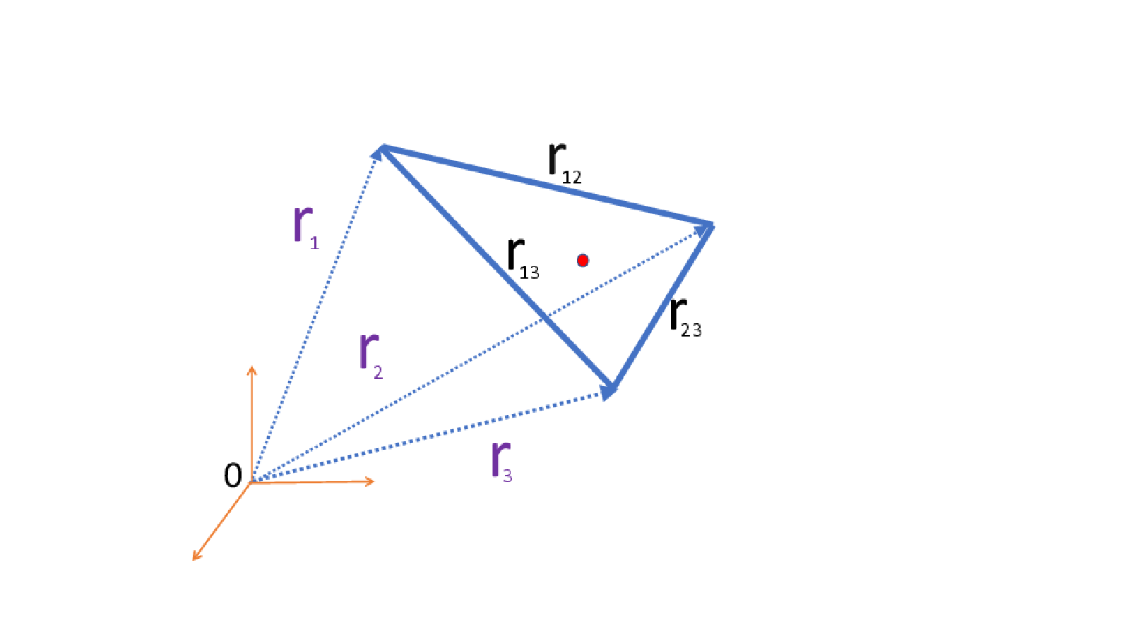
Refer to caption
Figure 1: Three-particle system: the coordinate vectors 𝐫i{\bf r}_{i} mark positions of vertices of the triangle of interaction with sides ri​jr_{ij}. The center-of-mass (the barycenter of the triangle) is marked by a (red) bubble.

The number of relative distances is equal to the number of edges of the triangle which is formed by taking the particle positions as vertices. We call this triangle the triangle of interaction, see for illustration Fig.1. Here, Δi(d)\Delta_{i}^{(d)} is the dd-dimensional Laplacian,

Δi(d)=∂2∂𝐫i​∂𝐫i,\Delta_{i}^{(d)}\ =\ \frac{\partial^{2}}{\partial{{\bf r}_{i}}\partial{{\bf r}_{i}}}\ ,

associated with the iith body. For simplicity all masses in (1) are assumed to be equal: mi=m=1m_{i}=m=1. The configuration space for ℋ{\cal H} is 𝐑3​d{\bf R}^{3d}. The center-of-mass motion described by vectorial coordinate

𝐑0=13∑k=13𝐫k,{\bf R}_{{}_{0}}\ =\ \frac{1}{{\sqrt{3}}}\,\sum_{k=1}^{3}{\bf r}_{{}_{k}}\ ,

can be separated out; this motion is described by a dd-dimensional plane wave, ∼ei𝐤⋅𝐑0\sim e^{i\,{\bf k}\cdot{\bf R}_{{}_{0}}}.

The spectral problem is formulated in the space of relative motion 𝐑r≡𝐑2​d{\bf R}_{r}\equiv{\bf R}^{2d}; it is of the form,

ℋr​Ψ​(x)≡(−12​Δr(2​d)+V⁡(r12,r13,r23))​Ψ​(x)=E​Ψ​(x),Ψ∈L2​(𝐑r),{\cal H}_{r}\,\Psi(x)\ \equiv\ \bigg(-\frac{1}{2}\,\Delta_{r}^{(2d)}+V(r_{12},\,r_{13},\,r_{23})\bigg)\,\Psi(x)\ =\ E\,\Psi(x)\ ,\ \Psi\in L_{2}({\bf R}_{r})\ , (3)

where Δr(2​d)\Delta_{r}^{(2d)} is the flat-space Laplacian in the space of relative motion. If the space of relative motion 𝐑r{\bf R}_{r} is parameterized by two, dd-dimensional vectorial Jacobi coordinates

𝐪j=1j⁡(j+1)∑k=1jk(𝐫k+1−𝐫k),j=1,2,{\bf q}_{j}\ =\ \frac{1}{\sqrt{j(j+1)}}\sum_{k=1}^{j}k\,({\bf r}_{k+1}-{\bf r}_{{k}})\ ,\qquad\qquad j=1,2\ , (4)

the flat-space 2​d2d-dimensional Laplacian in the space of relative motion becomes diagonal

Δr(2​d)=∑j=1,2∂2∂𝐪j​∂𝐪j.\Delta_{r}^{(2d)}\ =\ \sum_{j=1,2}\frac{\partial^{2}}{\partial{{\bf q}_{j}}\partial{{\bf q}_{j}}}\ . (5)

Thus, 𝐪j{\bf q}_{j} plays a role of the Cartesian coordinate vector in the space of relative motion.

The case d=1d=1 (three bodies on a line) is special. The triangle of interaction degenerates into an interval with the marked point inside - the vertices of the triangle correspond to the endpoints and the marked point - its area is equal to zero. Moreover, for d=1d=1 the relative distances obey the constraint (hyperplane condition),

r12+r23+r13= 0,r_{12}+r_{23}+r_{13}\ =\ 0\ , (6)

where it is assumed that r13=−r31r_{13}=-r_{31}. Hence, the three relative distances are related and only two relative distances can serve as independent variables. Therefore, the Laplacian in the space of relative variables becomes

Δr(2)= 2​(∂2∂r122+∂2∂r232−∂2∂r12​∂r23),\Delta_{r}^{(2)}\ =\ 2\,\bigg(\frac{\partial^{2}}{\partial r_{12}^{2}}\ +\ \frac{\partial^{2}}{\partial r_{23}^{2}}-\frac{\partial^{2}}{\partial r_{12}\,\partial r_{23}}\bigg)\ , (7)

cf. (5). The configuration space 𝐑r{\bf R}_{r} is the quadrant, r12,r23≥0r_{12},r_{23}\geq 0.

Observation [2] :

There exists a family of eigenstates of the Hamiltonian (1), including the ground state, which depend on the three relative distances {ri​j}\{r_{ij}\} alone . The same is correct for the nn body problem: there exists a family of eigenstates, including the ground state, which depend on relative distances alone.

This observation is presented for the case of scalar particles, bosons. It can be generalized to the case of fermions,

Conjecture :

In the case of three fermions there exists a family of the eigenstates of the Hamiltonian (1), including the ground state, in which the coordinate functions depend on three relative distances {ri​j}\{r_{ij}\} only . The same is correct for the nn body problem: there exists a family of the eigenstates, including the ground state, in which the coordinate functions depend on relative distances only.

Our primary goal is to find the differential operator in the space of relative distances {ri​j}\{r_{ij}\} for which these states are eigenstates. In other words, to find a differential equation depending only on {ri​j}\{r_{ij}\} for which these states are solutions. This implies a study of the evolution of the triangle of interaction with fixed barycenter (center-of-mass). We consider the case of three spinless particles.

In our previous paper [1] the physically important case d=3d=3 was studied in detail. In this paper it will be shown that the generalization to arbitrary dd is straightforward. Except for d=1d=1 almost all formulas remain conceptually unchanged, the presentation (and even wording) remains almost the same and most conclusions are unaltered.

I Generalities

As a first step let us change variables in the space of relative motion 𝐑r{\bf R}_{r}:

(𝐪j)↔(ri​j,Ω),({\bf q}_{j})\leftrightarrow(r_{ij},\Omega)\ ,

where for d>1d>1 the number of (independent) relative distances ri​jr_{ij} is equal to 3 and Ω\Omega is a collection of (2​d−3)(2d-3) angular variables. Thus, we split 𝐑r{\bf R}_{r} into a combination of the space of relative distances 𝐑~{\bf\tilde{R}} and a space parameterized by angular variables, essentially those on the sphere S2​d−3S^{2d-3}. There are known several ways to introduce variables in 𝐑r{\bf R}_{r}: the perimetric coordinates by Hylleraas [3], the scalar products of vectorial Jacobi coordinates 𝐫i​j{\bf r}_{ij} [4] and the three relative (mutual) distances ri​jr_{ij} (see e.g. [5]). We follow the last one. In turn, the angular variables are introduced as the Euler angles on the S2​d−4S^{2d-4} sphere defining the normal to the interaction plane (triangle) and the azimuthal angle of rotation of the interaction triangle around its barycenter, see e.g. [4].

A key observation is that in new coordinates (ri​j,Ω)(r_{ij},\Omega) the flat-space Laplace operator (the kinetic energy operator) in the space of relative motion 𝐑r{\bf R}_{r} takes the form of the sum of two second-order differential operators

12Δr(2​d)=ΔR(ri​j,∂i​j)+Δ~(ri​j,Ω,∂i​j,∂Ω),∂i​j≡∂∂ri​j,\frac{1}{2}\Delta_{r}^{(2d)}\ =\ {\Delta_{R}}(r_{ij},\partial_{ij})+{\tilde{\Delta}}(r_{ij},\Omega,\partial_{ij},\partial_{\Omega})\ ,\quad\partial_{ij}\equiv\frac{\partial}{\partial r_{ij}}\ , (8)

where the first operator depends on relative distances only, (hence, the coefficient functions do not depend on angles), while the second operator depends on angular derivatives in such a way that it annihilates any angle-independent function,

Δ~(ri​j,Ω,∂i​j,∂Ω)Ψ(ri​j)= 0.{\tilde{\Delta}}(r_{ij},\Omega,\partial_{ij},\partial_{\Omega})\,\Psi(r_{ij})\ =\ 0\ .

This observation holds for the nn-body case as well [6].

For d=1d=1 the operator Δ~{\tilde{\Delta}} is absent (no angular variables occur) and we have

ΔR(ri​j,∂i​j)=Δr(2),{\Delta_{R}}(r_{ij},\partial_{ij})\ =\ \Delta_{r}^{(2)}\ ,

see (7). In general, for d>1d>1 the commutator

[ΔR(ri​j),Δ~(ri​j,Ω,∂Ω)]≠0.[{\Delta_{R}}(r_{ij})\ ,\ {\tilde{\Delta}}(r_{ij},\Omega,\partial_{\Omega})]\neq 0\ .

If we look for angle-independent solutions of (3), due to the decomposition (8) the general spectral problem (3) reduces to a particular 3-body spectral problem

ℋ~RΨ(ri​j)≡(−ΔR(ri​j,∂i​j)+V(ri​j))Ψ(ri​j)=EΨ(ri​j),Ψ∈L2(𝐑~),{\tilde{\cal H}}_{R}\,\Psi(r_{ij})\ \equiv\ \bigg(-{\Delta_{R}}(r_{ij},\partial_{ij})+V(r_{ij})\bigg)\,\Psi(r_{ij})\ =\ E\,\Psi(r_{ij})\ ,\quad\Psi\in L_{2}({\bf\tilde{R}})\ , (9)

where 𝐑~{\bf\tilde{R}} is the space of relative distances. Clearly, we can write

ΔR(ri​j,∂i​j)=gμ​ν(r)∂μ∂ν+bμ∂μ,{\Delta_{R}}(r_{ij},\partial_{ij})\ =\ g^{\mu\nu}(r)\partial_{\mu}\partial_{\nu}\ +\ b^{\mu}\partial_{\mu}\ , (10)

where gμ​ν​(r)g^{\mu\nu}(r) is the matrix made out of coefficients in front of the second derivatives and bμb^{\mu} is a column vector.

Surprisingly, for any d>1d>1 one can find the dd-dependent gauge factor Γ⁡(ri​j)\Gamma(r_{ij}) such that the operator ΔR(ri​j,∂i​j){\Delta_{R}}(r_{ij},\partial_{ij}) takes the form of the Schrödinger operator,

Γ−1ΔR(ri​j,∂i​j)Γ=ΔL​B(r)−V~(r)≡−Δ~R,\Gamma^{-1}\,{\Delta_{R}}\,(r_{ij},\partial_{ij})\,\Gamma\ =\ {\Delta_{LB}}(r)-{\tilde{V}}(r)\ \equiv-{\tilde{\Delta}}_{R}\ , (11)

where ΔL​B​(r)\Delta_{LB}(r) is the Laplace-Beltrami operator with contravariant, dd-independent metric gμ​ν​(r)g^{\mu\nu}(r), in general, on some non-flat, (non-constant curvature) manifold. It makes sense of the kinetic energy. Here V~​(r){\tilde{V}}(r) is the effective potential. The potential V~{\tilde{V}} becomes singular at the boundary of the configuration space, where the determinant D⁡(r)=detgμ​ν​(r)D(r)=\det g^{\mu\nu}(r) vanishes. The operator Δ~R{\tilde{\Delta}}_{R} is Hermitian with measure D​(r)−12D(r)^{-\frac{1}{2}}. Eventually, we arrive at the spectral problem for the Hamiltonian

HL​B​(r)≡−ΔL​B​(r)+V⁡(r)+V~​(r),{H}_{LB}(r)\ \equiv\ -{\Delta_{LB}}(r)+V(r)+{\tilde{V}}(r)\ , (12)

with dd-independent kinetic energy ΔL​B​(r){\Delta_{LB}}(r). Again the case d=1d=1 is special, the gauge factor is trivial, Γ=1\Gamma=1, and

ΔL​B​(r)=ΔR​(r)=Δr(2).{\Delta_{LB}}(r)\ =\ {\Delta_{R}}(r)\ =\ \Delta_{r}^{(2)}\ .

Following the de-quantization procedure of replacement of the quantum momentum (derivative) by the classical momentum

−i∂→P,-i\,\partial\ \rightarrow\ P\ ,

one can get a classical analogue of (12),

HL​B(c)=gμ​ν​(r)​Pμ​Pν+V⁡(r)+V~​(r).{H}^{(c)}_{LB}\ =\ g^{\mu\nu}(r)P_{\mu}P_{\nu}+V(r)+{\tilde{V}}(r)\ . (13)

It describes the internal motion of a 3-dimensional body with tensor of inertia (gμ​ν)−1(g^{\mu\nu})^{-1}  with center of mass fixed.

The Hamiltonians (12), (13) are the main objects of study of this paper.

II Three-body case: d=1d=1, concrete results

In the one-dimensional case d=1d=1 the Laplace-Beltrami operator in (12) becomes

ΔL​B​(r)= 2​(∂2∂r122+∂2∂r232−∂2∂r12​∂r23),{\Delta_{LB}}(r)\ =\ 2\bigg(\frac{\partial^{2}}{\partial r_{12}^{2}}\ +\ \frac{\partial^{2}}{\partial r_{23}^{2}}-\frac{\partial^{2}}{\partial r_{12}\,\partial r_{23}}\bigg)\ ,

see (7). It corresponds to the two-dimensional flat space Laplacian and is evidently an algebraic operator. Formally, it is not S3S_{3} invariant unlike the original 3​d3d-Laplacian in (1), the kinetic energy, although it remains S2S_{2} invariant. Note that in variables,

r122=ρ12,r132=ρ13,r232=ρ23,r_{12}^{2}\ =\ \rho_{12}\ ,\ r_{13}^{2}\ =\ \rho_{13}\ ,\ r_{23}^{2}\ =\ \rho_{23}\ ,

see below, the emerging flat-space Laplacian ΔL​B​(ρ){\Delta_{LB}}(\rho) is not anymore algebraic. As a realization of S2S_{2} invariance of (7) let us introduce S2S_{2} invariants

ξ1=r12+r23,ξ2=r12​r23,\xi_{1}=r_{12}+r_{23}\quad,\quad\xi_{2}=r_{12}\,r_{23}\ , (14)

as new variables, which is a polynomial change of variables, then

ΔL​B​(ξ)= 2​(∂2∂ξ12+(ξ12−3​ξ2)​∂2∂ξ22+ξ1​∂2∂ξ1​∂ξ2−∂∂ξ2).{\Delta_{LB}}(\xi)\ =\ 2\,\bigg(\frac{\partial^{2}}{\partial\xi_{1}^{2}}\ +\ (\xi_{1}^{2}-3\xi_{2})\frac{\partial^{2}}{\partial\xi_{2}^{2}}+\xi_{1}\frac{\partial^{2}}{\partial\xi_{1}\,\partial\xi_{2}}-\frac{\partial}{\partial\xi_{2}}\bigg)\ . (15)

This is an algebraic operator which can be rewritten in terms of the generators of the maximal affine subalgebra b2b_{2} of the algebra s​l​(3,𝐑)sl(3,{\bf R}) in ξ\xi-variables, c.f. below (49), see [7, 8].

There exists another polynomial S2S_{2}-symmetric change of variables [8]

σ2=−r12​r23−r122−r232=ξ2−ξ12,σ3=−r12​r23​(r12+r23)=−ξ1​ξ2,\sigma_{2}=-r_{12}r_{23}-r_{12}^{2}-r_{23}^{2}\ =\ \xi_{2}-\xi_{1}^{2}\ ,\ \sigma_{3}=-r_{12}\,r_{23}(r_{12}+r_{23})=-\xi_{1}\xi_{2}\ , (16)

which leaves the operator ΔL​B{\Delta_{LB}} algebraic,

ΔL​B​(σ)=−2​(3​σ2​∂2∂σ22−σ22​∂2∂σ32+9​σ3​∂2∂σ2​∂σ3+3​∂∂σ2).{\Delta_{LB}}(\sigma)\ =\ -2\,\bigg(3\sigma_{2}\,\frac{\partial^{2}}{\partial\sigma_{2}^{2}}\ -\ \sigma_{2}^{2}\frac{\partial^{2}}{\partial\sigma_{3}^{2}}+9\,\sigma_{3}\frac{\partial^{2}}{\partial\sigma_{2}\,\partial\sigma_{3}}+3\frac{\partial}{\partial\sigma_{2}}\bigg)\ . (17)

In fact, the variables (16)

σ1=r12+r23+r31,σ2=r12r23+r12r13+r23r13,σ3=r12r23r13,\sigma_{1}=r_{12}+r_{23}+r_{31}\ ,\ \sigma_{2}=r_{12}r_{23}+r_{12}r_{13}+r_{23}r_{13}\quad,\quad\sigma_{3}=r_{12}\,r_{23}\,r_{13}\ , (18)

are S3S_{3} invariants, subject to the condition that the 1st invariant σ1\sigma_{1} vanishes,

σ1= 0.\sigma_{1}\ =\ 0\ .

Hence, the operator (17) is, in fact, S3S_{3} permutationally invariant. It can be immediately seen that the operator (17) describes the kinetic energy of relative motion of the 3-body (A2)(A_{2}) rational Calogero model [9] with potential

VA2=g⁡(1r122+1r232+1r132)=g⁡(1ρ12+1ρ23+1ρ13),V_{A_{2}}\ =\ g\bigg(\frac{1}{r_{12}^{2}}+\frac{1}{r_{23}^{2}}+\frac{1}{r_{13}^{2}}\bigg)\ =\ g\bigg(\frac{1}{\rho_{12}}+\frac{1}{\rho_{23}}+\frac{1}{\rho_{13}}\bigg)\ , (19)

in algebraic form, see [8]. It is easy to check that the potential VA2V_{A_{2}} is a rational function in σ2,3\sigma_{2,3} (16). It was shown in [7, 8] that the Hamiltonian of relative motion of the 3-body (A2)(A_{2}) rational Calogero model (even with potential modified by adding the harmonic oscillator potential), gauge-rotated with its ground state function and written in variables σ2,3\sigma_{2,3} is an algebraic operator as well. This operator can be rewritten in terms of the generators of the maximal affine subalgebra b2b_{2} of the algebra s​l​(3,𝐑)sl(3,{\bf R})

𝒥i−\displaystyle{\cal J}_{i}^{-} =\displaystyle= ∂∂ui,i=1,2,\displaystyle\frac{\partial}{\partial u_{i}}\ ,\qquad\quad i=1,2\ ,
𝒥i​j0\displaystyle{{\cal J}_{ij}}^{0} =\displaystyle= ui​∂∂uj,i,j=1,2,\displaystyle u_{i}\frac{\partial}{\partial u_{j}}\ ,\qquad i,j=1,2\ , (20)
𝒥0​(N)\displaystyle{\cal J}^{0}(N) =\displaystyle= ∑i=12ui​∂∂ui−N,\displaystyle\sum_{i=1}^{2}u_{i}\frac{\partial}{\partial u_{i}}-N\,,
𝒥i+​(N)\displaystyle{\cal J}_{i}^{+}(N) =\displaystyle= ui𝒥0(N)=ui(∑j=12uj∂∂uj−N),i=1,2,\displaystyle u_{i}{\cal J}^{0}(N)\ =\ u_{i}\,\left(\sum_{j=1}^{2}u_{j}\frac{\partial}{\partial u_{j}}-N\right)\ ,\quad i=1,2\ , (21)

where NN is a parameter and

u1=σ2,u2=σ3.u_{1}\ =\ \sigma_{2}\ ,\ u_{2}\ =\ \sigma_{3}\ .

Another polynomial change of variables

λ1=σ2=−r12​r23−r122−r232=ξ2−ξ12,λ2=σ32=r122​r232​(r12+r23)2=ξ12​ξ22,\lambda_{1}=\sigma_{2}=-r_{12}r_{23}-r_{12}^{2}-r_{23}^{2}\ =\ \xi_{2}-\xi_{1}^{2}\ ,\ \lambda_{2}=\sigma_{3}^{2}=r_{12}^{2}\,r_{23}^{2}(r_{12}+r_{23})^{2}=\xi_{1}^{2}\xi_{2}^{2}\ , (22)

leaves the operator ΔL​B{\Delta_{LB}} algebraic,

ΔL​B​(λ)=−2​(3​λ1​∂2∂λ12− 4​λ12​λ2​∂2∂λ22+18​λ2​∂2∂λ1​∂λ2+3​∂∂λ1−2​λ12​∂∂λ2).{\Delta_{LB}}(\lambda)\ =\ -2\,\bigg(3\lambda_{1}\,\frac{\partial^{2}}{\partial\lambda_{1}^{2}}\ -\ 4\lambda_{1}^{2}\lambda_{2}\frac{\partial^{2}}{\partial\lambda_{2}^{2}}+18\,\lambda_{2}\frac{\partial^{2}}{\partial\lambda_{1}\,\partial\lambda_{2}}+3\frac{\partial}{\partial\lambda_{1}}-2\lambda_{1}^{2}\frac{\partial}{\partial\lambda_{2}}\bigg)\ . (23)

It can be immediately seen that the operator (23) describes the kinetic energy of relative motion of the 3-body (G2)(G_{2}) rational Wolfes model [10] with potential

VG2=g⁡(1r122+1r232+1r132)+g1​(1(r12−r23)2+1(r23−r31)2+1(r12−r31)2),V_{G_{2}}\ =\ g\bigg(\frac{1}{r_{12}^{2}}+\frac{1}{r_{23}^{2}}+\frac{1}{r_{13}^{2}}\bigg)\ +\ g_{1}\bigg(\frac{1}{(r_{12}-r_{23})^{2}}+\frac{1}{(r_{23}-r_{31})^{2}}+\frac{1}{(r_{12}-r_{31})^{2}}\bigg)\ ,

in algebraic form, see [8]. It can be rewritten in terms of the generators of the algebra g(2)g^{(2)}, see [8]. It is easy to check that the potential VG2V_{G_{2}} is a rational function in λ1,2\lambda_{1,2} (22). It was shown in [7, 8] that the Hamiltonian of relative motion of the 3-body (G2)(G_{2}) rational Wolfes model (even with potential modified by adding the harmonic oscillator potential), gauge-rotated with its ground state function and written in variables λ1,2\lambda_{1,2} is an algebraic operator. This operator can also be rewritten in terms of the generators of the algebra g(2)g^{(2)}.

The most general polynomial change of variables known so far, which leaves the operator ΔL​B{\Delta_{LB}} algebraic, has led to the discovery of the so-called TTW model [11] - the most general superintegrable and exactly-solvable model on the plane. Following Calogero [9] let us introduce polar coordinates in the space of relative distances,

q1=12​r12=r​cos⁡φ,q2=23​(r13+r23)=r​sin⁡φ,q_{1}\,=\,\frac{1}{\sqrt{2}}\,r_{12}=r\cos\varphi\ ,\ q_{2}\,=\,\sqrt{\frac{2}{3}}\,(r_{13}+r_{23})=r\sin\varphi\ ,

see (4). Now we define new variables

t=r2,u=r2​k​sin2⁡k​φ,t\ =\ r^{2}\ ,\ u\ =\ r^{2k}\sin^{2}{k\varphi}\ ,

which are the invariants of the dihedral group I2​(k)I_{2}(k) for integer kk  (and even rational kk). The operator (7) takes an amazingly simple algebraic form,

ΔL​B(k)=−4t∂2t−8ku∂2t​u−4k2tk−1u∂2u−4∂t−2k2tk−1∂u,{\Delta_{LB}}^{(k)}\ =\ -4t\partial^{2}_{t}-8ku\partial^{2}_{tu}-4k^{2}t^{k-1}u\partial^{2}_{u}-4\partial_{t}-2k^{2}t^{k-1}\partial_{u}\ ,

for k=1,2,…k=1,2,\ldots . This operator can be rewritten in terms of the generators of the algebra g(k)g^{(k)}, see [11] . Forming the Schrödinger operator

ℋT​T​W(k)=−ΔL​B(k)+ω2​t+k2​α​tk−1tk−u+k2​β​tk−1u,{\cal H}_{TTW}^{(k)}\ =\ -{\Delta_{LB}}^{(k)}+\omega^{2}t+\frac{k^{2}\alpha\,t^{k-1}}{t^{k}-u}+\frac{k^{2}\beta\,t^{k-1}}{u}\ , (24)

we arrive at the Tremblay-Turbiner-Winternitz (TTW) model; if k=3k=3 at α=0\alpha=0 the 3-body (A2)(A_{2}) rational Calogero model occurs, otherwise for α≠0\alpha\neq 0 the 3-body (G2)(G_{2}) rational Wolfes model occurs, both after separation out center-of-mass motion. Interestingly, for k=1k=1 we get the Smorodinsky-Winternitz model, while for k=2k=2 it will be the B​C2BC_{2} rational model. Both models describe the relative motion of 3-body problem.

The TTW model is exactly-solvable and integrable for any real kk - there exists a 2nd order integral (the 1st order symmetry operator squared), while for rational k=p/qk=p/q the model is superintegrable - there exists an integral of order 2​(p+q)−12(p+q)-1 [12]. For integer kk by gauge-rotation of the Hamiltonian (24) with its ground state function one can transform it to an algebraic operator. The same is true for both integrals: gauge rotation with ground state eigenfunction leads them to a form of algebraic operators in variables t,ut,u . All these algebraic operators can be rewritten in terms of the generators of the algebra g(k)g^{(k)}.

It must be emphasized that there are non-polynomial changes of variables (r12,r23)(r_{12}\,,\,r_{23}) (trigonometric and elliptic) in ( 7) which can still lead to algebraic operators. In the case of trigonometric change of variables there occurs the kinetic energy of the relative motion of 3-body, (A2)(A_{2}) trigonometric Sutherland model [7], or (G2)(G_{2}) trigonometric Sutherland model [8], or the kinetic energy of B​C2BC_{2} trigonometric model [13]. For discussion see [14].

In the case of elliptic change of variables there occurs the kinetic energy of relative motion of the 3-body, (A2)(A_{2}) elliptic Calogero model, or (G2)(G_{2}) elliptic model [15], or the kinetic energy of the B​C2BC_{2} elliptic model [16].

III Three-body case: d>1d>1, concrete results

III.1 rr-representation

Assuming d>1d>1, after straightforward calculations the operator ΔR(ri​j,∂i​j){\Delta_{R}}(r_{ij},\partial_{ij}) (in decomposition (8)) can be found to be

2ΔR(ri​j,∂i​j)=[ 2(∂r122+∂r232+∂r132)+2​(d−1)r12∂r12+2​(d−1)r23∂r23+2​(d−1)r13∂r132{\Delta_{R}}(r_{ij},\partial_{ij})\ =\ \bigg[\ 2\,(\partial^{2}_{r_{12}}+\partial^{2}_{r_{23}}+\partial^{2}_{r_{13}})+\frac{2(d-1)}{r_{12}}\,\partial_{r_{12}}+\frac{2(d-1)}{r_{23}}\,\partial_{r_{23}}+\frac{2(d-1)}{r_{13}}\,\partial_{r_{13}}
+r122−r132+r232r12​r23∂r12∂r23+r122+r132−r232r12​r13∂r12∂r13+r132+r232−r122r13​r23∂r23∂r13],+\frac{r_{12}^{2}-r_{13}^{2}+r_{23}^{2}}{r_{12}r_{23}}\,\partial_{r_{12}}\partial_{r_{23}}+\frac{r_{12}^{2}+r_{13}^{2}-r_{23}^{2}}{r_{12}r_{13}}\,\partial_{r_{12}}\partial_{r_{13}}+\frac{r_{13}^{2}+r_{23}^{2}-r_{12}^{2}}{r_{13}r_{23}}\,\partial_{r_{23}}\partial_{r_{13}}\ \bigg]\ , (25)

cf. e.g. [5]. Note that at d=1d=1 the operator (25) becomes degenerate. This can be seen by calculating the determinant of the metric gμ​νg^{\mu\nu}, see (10) for definition, of the operator (25),

D⁡(r)=detgμ​ν​(r)=12r122​r232​r132​(r122+r232+r132)​S△2,D(r)=\det g^{\mu\nu}(r)\ =\ \frac{12}{r_{12}^{2}\,r_{23}^{2}\,r_{13}^{2}}(r_{12}^{2}+r_{23}^{2}+r_{13}^{2})\,S^{2}_{\triangle}\ ,

where S△S_{\triangle} is the area of the interaction triangle, see below. For d=1d=1 the interaction triangle shrinks to the interval with marked point, its area vanishes, S△=0S_{\triangle}=0, and the determinant is identically zero, D⁡(r)=0D(r)=0. This implies that the original three-dimensional configuration space at d>1d>1 given by S△≥0S_{\triangle}\geq 0, shrinks to the boundary, S△=0S_{\triangle}=0 and effectively becomes two-dimensional.

In general, the operator (25) does not depend on the choice of the angular variables Ω\Omega. While the operator Δ~(ri​j,∂i​j,Ω,∂Ω){\tilde{\Delta}}(r_{ij},\partial_{ij},\Omega,\partial_{\Omega}) in (8), for example at d=2d=2, where there is a single angular variable, Ω=θ\Omega=\theta, is equal to

Δ~=−12​S△r122​r232​r132(r123∂r12+r233∂r23+r133∂r13−r124+r234+r134S△∂θ)∂θ,{\tilde{\Delta}}\ =\ -\ \frac{12\,S_{\triangle}}{r_{12}^{2}\,r_{23}^{2}\,r_{13}^{2}}\,\bigg({r_{12}^{3}}\,\partial_{r_{12}}\,+\,{r_{23}^{3}}\,\partial_{r_{23}}\,+\,{r_{13}^{3}}\,\partial_{r_{13}}\,-\,\frac{r_{12}^{4}+r_{23}^{4}+r_{13}^{4}}{S_{\triangle}}\,\partial_{\theta}\bigg)\partial_{\theta}\ ,

where θ\theta is the azimuthal angle of rotation around barycenter of triangle of interaction, see Fig. 1 and S△S_{\triangle} is the area of the interaction triangle, see below Eq.(29). It is evident that Δ~{\tilde{\Delta}} annihilates any angle-independent function. The variable θ\theta is not separated in Δ~{\tilde{\Delta}} and, thus, in Δr(2​d)\Delta_{r}^{(2d)} (8): the eigenfunctions in (3) are not factorizable to the form R⁡(ri​j)​A​(θ)R(r_{ij})\,A(\theta).

The configuration space in the space of relative distances is

0<r12,r13,r23<∞,r23<r12+r13,r13<r12+r23,r12<r13+r23,0<r_{12},r_{13},r_{23}<\infty\,,\quad r_{23}<\ r_{12}+r_{13}\,,\quad r_{13}<r_{12}+r_{23}\,,\quad r_{12}<r_{13}+r_{23}\ , (26)

equivalent to S△>0S_{\triangle}>0. In the space with Cartesian coordinates (x,y,z)=(r12,r13,r23)(x,y,z)=(r_{12},r_{13},r_{23}) the configuration space lies in the first octant and is the interior of the inverted tetrahedral-shaped object with base at infinity, vertex at the origin and edges (t,t,2​t)(t,t,2t), (t,2​t,t)(t,2t,t) and (2​t,t,t)(2t,t,t), 0≤t<∞0\leq t<\infty.

III.2 ρ\rho-representation

Formally, the operator (25) is invariant under reflections Z2⊕Z2⊕Z2Z_{2}\oplus Z_{2}\oplus Z_{2},

r12→−r12,r13⇔−r13,r23⇔−r23,r_{12}\rightarrow-r_{12}\ ,\qquad r_{13}\Leftrightarrow-r_{13}\ ,\qquad r_{23}\Leftrightarrow-r_{23}\ ,

and w.r.t. S3S_{3}-group action. If we introduce new variables,

r122=ρ12,r132=ρ13,r232=ρ23,r_{12}^{2}\ =\ \rho_{12}\ ,\ r_{13}^{2}\ =\ \rho_{13}\ ,\ r_{23}^{2}\ =\ \rho_{23}\ , (27)

the operator (25) becomes algebraic,

ΔR(ρ)= 4(ρ12∂ρ122+ρ13∂ρ132+ρ23∂ρ232)+{\Delta_{R}}(\rho)\ =\ 4(\rho_{12}\partial^{2}_{\rho_{12}}+\rho_{13}\partial^{2}_{\rho_{13}}+\rho_{23}\partial^{2}_{\rho_{23}})\ +\
2((ρ12+ρ13−ρ23)∂ρ12∂ρ13+(ρ12+ρ23−ρ13)∂ρ12∂ρ23+(ρ13+ρ23−ρ12)∂ρ13∂ρ23)+2\bigg((\rho_{12}+\rho_{13}-\rho_{23})\partial_{\rho_{12}}\partial_{\rho_{13}}\ +(\rho_{12}+\rho_{23}-\rho_{13})\partial_{\rho_{12}}\partial_{\rho_{23}}\ +(\rho_{13}+\rho_{23}-\rho_{12})\partial_{\rho_{13}}\partial_{\rho_{23}}\bigg)\ +
2d(∂ρ12+∂ρ13+∂ρ23),2d(\partial_{\rho_{12}}+\partial_{\rho_{13}}+\partial_{\rho_{23}})\ , (28)

c.f. [1] at d=3d=3. Note that the operator (28) is of Lie-algebraic nature: it can be rewritten in terms of the generators of the algebra s​l​(4,𝐑)sl(4,{\bf R}) realized by the first order differential operators, see below. It acts as a filtration for the flag of finite-dimensional representation spaces of this algebra

𝒫N(1,2,3)=⟨ρ12p1ρ13p2ρ23p3| 0≤p1+p2+p3≤N⟩,N=0,1,2,….{\mathcal{P}}^{(1,2,3)}_{N}\ =\ \langle\rho_{12}^{p_{1}}\rho_{13}^{p_{2}}\rho_{23}^{p_{3}}|\ 0\leq p_{1}+p_{2}+p_{3}\leq N\rangle\ ,\ N=0,1,2,\ldots\ .

From (26) and (27) it follows that the corresponding configuration space in ρ\rho variables is given by the conditions

0<ρ12,ρ13,ρ23<∞,ρ23<(ρ12+ρ13)2,ρ13<(ρ12+ρ23)2,ρ12<(ρ13+ρ23)2,0<\rho_{12},\rho_{13},\rho_{23}<\infty\ ,\ {\rho}_{23}<(\sqrt{{\rho}_{12}}+\sqrt{{\rho}_{13}})^{2},\ {\rho}_{13}<(\sqrt{{\rho}_{12}}+\sqrt{{\rho}_{23}})^{2},\ {\rho}_{12}<\ (\sqrt{{\rho}_{13}}+\sqrt{{\rho}_{23}})^{2}\ ,

equivalent to S△>0S_{\triangle}>0. The boundary of the configuration space is given by S⁡(ρ)=S△2=0S(\rho)=S^{2}_{\triangle}=0. We remark that

−16​S≡ρ122+ρ132+ρ232−2​(ρ12​ρ13+ρ12​ρ23+ρ13​ρ23)≤ 0,\quad-16\,S\ \equiv\ \rho_{12}^{2}+\rho_{13}^{2}+\rho_{23}^{2}-2(\rho_{12}\rho_{13}+\rho_{12}\rho_{23}+\rho_{13}\rho_{23})\ \leq\ 0\ , (29)

because the left-hand side (l.h.s.) is equal to

−(r12+r13−r23)​(r12+r23−r13)​(r13+r23−r12)​(r12+r13+r23)-(r_{12}+r_{13}-r_{23})(r_{12}+r_{23}-r_{13})(r_{13}+r_{23}-r_{12})(r_{12}+r_{13}+r_{23})

and conditions (26) should hold. Therefore, following the Heron formula, l.h.s. is proportional to the square of the area of the triangle of interaction S△2=SS^{2}_{\triangle}=S .

The associated contravariant metric for the operator ΔR​(ρ){\Delta_{R}}(\rho) defined by coefficients in front of second derivatives is remarkably simple

gμ​ν​(ρ)=|4​ρ12ρ12+ρ13−ρ23ρ12+ρ23−ρ13ρ12+ρ13−ρ23 4​ρ13ρ13+ρ23−ρ12ρ12+ρ23−ρ13ρ13+ρ23−ρ124​ρ23|,g^{\mu\nu}(\rho)\ =\left|\begin{array}[]{ccc}4\rho_{12}&\ \rho_{12}+\rho_{13}-\rho_{23}&\ \rho_{12}+\rho_{23}-\rho_{13}\\ &&\\ \rho_{12}+\rho_{13}-\rho_{23}&\ 4\rho_{13}&\ \rho_{13}+\rho_{23}-\rho_{12}\\ &&\\ \rho_{12}+\rho_{23}-\rho_{13}&\ \rho_{13}+\rho_{23}-\rho_{12}&4\rho_{23}\end{array}\right|\ , (30)

it is linear in ρ\rho-coordinates(!) with factorized determinant

detgμ​ν​(ρ)=−6​(ρ12+ρ13+ρ23)​(ρ122+ρ132+ρ232−2​(ρ12​ρ13+ρ12​ρ23+ρ13​ρ23))≡D⁡(ρ)≥0,\det g^{\mu\nu}(\rho)\ =\ -6\left(\rho_{12}+\rho_{13}+\rho_{23}\right)\left(\rho_{12}^{2}+\rho_{13}^{2}+\rho_{23}^{2}-2(\rho_{12}\,\rho_{13}+\rho_{12}\,\rho_{23}+\rho_{13}\,\rho_{23})\,\right)\equiv D(\rho)\geq 0\ , (31)

and is positive definite. It does not depend on dimension dd, c.f. [1], explicitly. However, at d=1d=1 this determinant vanishes identically(!) (see below). It is worth noting a remarkable factorization property of the determinant

D(ρ)= 6(r122+r132+r232)×D(\rho)\ =\ 6\,(r_{12}^{2}+r_{13}^{2}+r_{23}^{2})\ \times
(r12+r13−r23)​(r12+r23−r13)​(r13+r23−r12)​(r12+r13+r23)=(r_{12}+r_{13}-r_{23})(r_{12}+r_{23}-r_{13})(r_{13}+r_{23}-r_{12})(r_{12}+r_{13}+r_{23})\ =
= 96​P​S△2,=\ 96\,P\ S^{2}_{\triangle}\ ,

where P=r122+r132+r232P=r_{12}^{2}+r_{13}^{2}+r_{23}^{2} - the sum of squares of the sides of the interaction triangle - the trace of metric tensor, Tr​gμ​ν​(ρ)=P/4\mbox{Tr}\,g^{\mu\nu}(\rho)=P/4\,.

The operator (28) is S3S_{3} permutationally-invariant. Hence, it can be rewritten in terms of elementary symmetric polynomials σ1,2,3\sigma_{1,2,3},

τ1=σ1​(ρ12,ρ13,ρ23)=ρ12+ρ13+ρ23,\displaystyle\tau_{1}\ =\ \sigma_{1}(\rho_{12},\,\rho_{13},\,\rho_{23})\ =\ \rho_{12}+\rho_{13}+\rho_{23}\ , (32)
τ2=σ2​(ρ12,ρ13,ρ23)=ρ12​ρ13+ρ12​ρ23+ρ13​ρ23,\displaystyle\tau_{2}\ =\ \sigma_{2}(\rho_{12},\,\rho_{13},\,\rho_{23})\ =\ \rho_{12}\,\rho_{13}+\rho_{12}\,\rho_{23}+\rho_{13}\,\rho_{23}\ ,
τ3=σ3​(ρ12,ρ13,ρ23)=ρ12​ρ13​ρ23.\displaystyle\tau_{3}\ =\ \sigma_{3}(\rho_{12},\,\rho_{13},\,\rho_{23})\ =\ \rho_{12}\,\rho_{13}\,\rho_{23}\ .

The determinant D⁡(ρ)D(\rho) has the very simple form,

D⁡(ρ)= 6​τ1​(4​τ2−τ12),D(\rho)\ =\ 6\,\tau_{1}\ (4\tau_{2}-\tau_{1}^{2})\ , (33)

with

16​S△2=(4​τ2−τ12),16\,S^{2}_{\triangle}\ =\ (4\,\tau_{2}-\tau_{1}^{2})\ ,

where only the elementary symmetric polynomials τ1,2\tau_{1,2} are involved. When detgμ​ν​(ρ)=0\det g^{\mu\nu}(\rho)=0, hence, either τ1=0\tau_{1}=0, or τ12=4​τ2\tau_{1}^{2}=4\tau_{2}, it defines the boundary of the configuration space, see (29).

III.3 τ\tau-representation

The operator (28) being rewritten in terms of elementary symmetric polynomials σ1,2,3\sigma_{1,2,3} in ρ\rho-variables (32), remains algebraic

ΔR(τ)= 6τ1∂τ12+ 2τ1(7τ2−τ12)∂τ22+ 2τ3(6τ2−τ12)∂τ32+ 24τ2∂1,22+ 36τ3∂τ1,τ32{\Delta_{R}}(\tau)\ =\ 6\,\tau_{1}\partial_{\tau_{1}}^{2}\ +\ 2\tau_{1}(7\tau_{2}-\tau_{1}^{2})\partial_{\tau_{2}}^{2}\ +\ 2\tau_{3}(6\tau_{2}-\tau_{1}^{2})\partial_{\tau_{3}}^{2}\ +\ 24\,\tau_{2}\partial_{1,2}^{2}\ +\ 36\tau_{3}\partial_{{\tau_{1}},{\tau_{3}}}^{2}
+ 2[9τ3τ1+τ2(4τ2−τ12)]∂τ2,τ32+ 6d∂τ1+ 2(2d+1)τ1∂τ2+ 2[(d+4)τ2−τ12]∂τ3,\ +\ 2\,[9\tau_{3}\tau_{1}+\tau_{2}(4\,\tau_{2}-\tau_{1}^{2})]\partial_{{\tau_{2}},{\tau_{3}}}^{2}\ +\ 6\,d\,\partial_{\tau_{1}}\ +\ 2\,(2d+1)\tau_{1}\,\partial_{\tau_{2}}\ +\ 2\,[(d+4)\tau_{2}-\tau_{1}^{2}]\,\partial_{\tau_{3}}\ , (34)

with metric

gμ​ν​(τ)=|6​τ112​τ218​τ312​τ22​τ1​(7​τ2−τ12) 9​τ3​τ1+4​τ22−τ2​τ1218​τ3 9​τ3​τ1+4​τ22−τ2​τ122​τ3​(6​τ2−τ12)|,g^{\mu\nu}(\tau)\ =\left|\begin{array}[]{ccc}6\,\tau_{1}&12\,\tau_{2}&18\,\tau_{3}\\ &&\\ 12\,\tau_{2}&2\,\tau_{1}\,(7\,\tau_{2}-\tau_{1}^{2})&\ 9\,\tau_{3}\,\tau_{1}+4\,\tau_{2}^{2}-\tau_{2}\,\tau_{1}^{2}\\ &&\\ 18\,\tau_{3}&\ 9\,\tau_{3}\,\tau_{1}+4\,\tau_{2}^{2}-\tau_{2}\tau_{1}^{2}&2\,\tau_{3}\,(6\,\tau_{2}-\tau_{1}^{2})\end{array}\right|\ , (35)

see below (72), (73). Its determinant,

detgμ​ν​(τ)= 6​τ1​(4​τ2−τ12)​[2​τ1​(9​τ2−2​τ12)​τ3−(4​τ2−τ12)−27​τ33],\det g^{\mu\nu}(\tau)\ =\ 6\,\tau_{1}\,\left(4\tau_{2}-\tau_{1}^{2}\right)[2\,\tau_{1}\,(9\,\tau_{2}-2\,\tau_{1}^{2})\,\tau_{3}-(4\,\tau_{2}-\tau_{1}^{2})-27\,\tau_{3}^{3}]\ ,

c.f. (33). Again, the determinant vanishes, if (16​S△2)=(4​τ2−τ12)=0(16\,S^{2}_{\triangle})=({4\tau_{2}-\tau_{1}^{2}})=0.

III.4 Geometrical variables representation

It is important to point out that the operator ΔR​(τ){\Delta_{R}}(\tau) can be rewritten in geometrical terms using them as geometrical variables

P=τ1=ρ12+ρ13+ρ23,\displaystyle P\ =\ \tau_{1}\ =\ \rho_{12}\ +\ \rho_{13}\ +\ \rho_{23}\ , (36)
S=S△2=4​τ2−τ1216=2​(ρ12​ρ13+ρ12​ρ23+ρ13​ρ23)−(ρ122+ρ132+ρ232)16,\displaystyle S\ =\ S^{2}_{\triangle}\ =\ \frac{4\,\tau_{2}-\tau_{1}^{2}}{16}\ =\ \frac{2(\rho_{12}\,\rho_{13}+\rho_{12}\,\rho_{23}+\rho_{13}\,\rho_{23})-(\rho_{12}^{2}+\rho_{13}^{2}+\rho_{23}^{2})}{16}\ ,
T=τ3=ρ12​ρ13​ρ23,\displaystyle T=\tau_{3}\ =\ \rho_{12}\,\rho_{13}\,\rho_{23}\ ,

namely,

ΔR=\displaystyle\Delta_{R}\ = 6P∂2P+12PS∂S2+T(48S+P2)∂T2+36T∂P,T+24S∂P,S+2S(16S+P2)∂S,T\displaystyle 6\,P\,\partial^{2}_{P}+\frac{1}{2}\,P\,S\,\partial_{S}^{2}+T\,(48\,S+P^{2})\,\partial_{T}^{2}+36\,T\,\partial_{P,{T}}+24\,S\,\partial_{P,S}+2\,S(16\,S+P^{2})\,\partial_{S,{T}} (37)
+ 6d∂P+14(d−1)P∂S+[8(d+4)S+d2P2]∂T,\displaystyle+\ 6\,d\,\partial_{P}\ +\ \frac{1}{4}\,(d-1)\,P\,\partial_{S}\ +\ [8\,(d+4)\,S+\frac{d}{2}\,P^{2}]\,\partial_{T}\ ,

where the metric is of the form

gμ​ν=|6​P 12​S 18​T12​S12​P​SS⁡(16​S+P2)18​TS⁡(16​S+P2)τ3​(48​S+P2)|,g^{\mu\nu}\ =\left|\begin{array}[]{ccc}6\,P&\ 12\,S&\ 18\,T\\ 12\,S&\ \frac{1}{2}P\,S&\ S(16\,S+P^{2})\\ 18\,T&\ S(16\,S+P^{2})&\ \tau_{3}(48\,S+P^{2})\\ \end{array}\right|\ , (38)

with determinant

detgμ​ν=−3​P​S​( 54​T2−T​P​(P2+ 144​S)+ 2​S​(P2+16​S)2).\det g^{\mu\nu}\ =\ -3\,P\,S\,\left(\ 54\,T^{2}\ -\ T\,P\left(P^{2}\,+\,144\,\,S\right)\ +\ 2\,S\,\left(P^{2}+16\,S\right)^{2}\ \right)\ .

Note that the operator (37) is of Lie-algebraic nature: it can be rewritten in terms of the generators of the algebra h(3)h^{(3)} realized by the differential operators, see below. It acts as a filtration for the flag of finite-dimensional representation spaces of this algebra

𝒫N(1,2,3)=⟨Pp1Sp2Tp3| 0≤p1+2p2+3p3≤N⟩,N=0,1,2,….{\mathcal{P}}^{(1,2,3)}_{N}\ =\ \langle P^{p_{1}}S^{p_{2}}T^{p_{3}}|\ 0\leq p_{1}+2p_{2}+3p_{3}\leq N\rangle\ ,\ N=0,1,2,\ldots\ .

This operator will be instrumental for construction of (quasi)-exactly-solvable problems for Case III.

III.5 Towards d=1d=1

For d=1d=1 when the square of the interaction triangle vanishes, hence, S≡116​(4​τ2−τ12)=0S\equiv\frac{1}{16}(4\tau_{2}-\tau_{1}^{2})=0, the metric becomes degenerate, detgμ​ν​(ρ)=detgμ​ν​(τ)=0\det g^{\mu\nu}(\rho)=\det g^{\mu\nu}(\tau)=0. Effectively, it leads to a reduction of the dimension of the space of relative distances from 3 to 2: the configuration space 4​τ2−τ12≥04\tau_{2}-\tau_{1}^{2}\geq 0 shrinks to the boundary 4​τ2−τ12=04\tau_{2}-\tau_{1}^{2}=0. In order to see this dimensional reduction explicitly, let us change variables in (28),

(ρ12,ρ13,ρ23)→(ρ12,ρ13,S).(\rho_{12},\rho_{13},\rho_{23})\rightarrow(\rho_{12},\rho_{13},S)\ .

It follows that

ΔR(ρ)= 4(ρ12∂ρ122+ρ13∂ρ132)+12S(ρ12+ρ13+ρ23)∂S2+ 2(ρ12+ρ13−ρ23)∂ρ12∂ρ13+{\Delta_{R}}(\rho)\ =\ 4(\rho_{12}\partial^{2}_{\rho_{12}}+\rho_{13}\partial^{2}_{\rho_{13}})+\frac{1}{2}\,S\,(\rho_{12}+\rho_{13}+\rho_{23})\partial^{2}_{S}\ +\ 2(\rho_{12}+\rho_{13}-\rho_{23})\partial_{\rho_{12}}\partial_{\rho_{13}}\ +
8S(∂ρ12∂S+∂ρ13∂S)+ 2d(∂ρ12+∂ρ13)+14(d−1)(ρ12+ρ13+ρ23)∂S,8\,S\,(\partial_{\rho_{12}}\partial_{S}\ +\ \partial_{\rho_{13}}\partial_{S})\ +\ 2d(\partial_{\rho_{12}}+\partial_{\rho_{13}})+\frac{1}{4}(d-1)(\rho_{12}+\rho_{13}+\rho_{23})\partial_{S}\ , (39)

with metric

gμ​ν=|4​ρ12 4​Sρ12+ρ13−ρ234​S12​S​(ρ12+ρ13+ρ23) 4​Sρ12+ρ13−ρ23 4​S 4​ρ13|,g^{\mu\nu}\ =\left|\begin{array}[]{ccc}4\,\rho_{12}&\ 4\,S&\ \rho_{12}+\rho_{13}-\rho_{23}\\ 4\,S&\ \frac{1}{2}\,S\,(\rho_{12}+\rho_{13}+\rho_{23})&\ 4\,S\\ \rho_{12}+\rho_{13}-\rho_{23}&\ 4\,S&\ 4\,\rho_{13}\\ \end{array}\right|\ , (40)

where ρ23=ρ23​(ρ12,ρ13,S){\rho}_{23}={\rho}_{23}({\rho}_{12},{\rho}_{13},S) and determinant

detgμ​ν=−12​S​(4​S−ρ12​ρ13)​ρ23,\det g^{\mu\nu}\ =\ -12\,S\,(4\,S-\rho_{12}\,\rho_{13})\,{\rho}_{23}\ ,

which vanishes identically if S=0S=0.

Imposing conditions: d=1d=1 and S=0S=0 on ΔR\Delta_{R} (39), we get

Δ~R(ρ)= 4(ρ12∂ρ122+ρ13∂ρ132)+ 2(ρ12+ρ13−ρ23)∂ρ12∂ρ13+ 2(∂ρ12+∂ρ13),{{\tilde{\Delta}}_{R}}(\rho)\ =\ 4(\rho_{12}\partial^{2}_{\rho_{12}}+\rho_{13}\partial^{2}_{\rho_{13}})\ +\ 2(\rho_{12}+\rho_{13}-\rho_{23})\partial_{\rho_{12}}\partial_{\rho_{13}}\ +\ 2(\partial_{\rho_{12}}+\partial_{\rho_{13}})\ , (41)

where ρ23=(ρ12±ρ13)2{\rho}_{23}=(\sqrt{{\rho}_{12}}\pm\sqrt{{\rho}_{13}})^{2} . The operator (41) is not algebraic anymore. However, it can be easily checked by calculating the curvature that is a Laplace-Beltrami operator in flat space. By changing variables ρ→r\rho\rightarrow r in (41),

r122=ρ12,r132=ρ13,r_{12}^{2}\ =\ \rho_{12}\ ,\ r_{13}^{2}\ =\ \rho_{13}\ ,

we arrive at the algebraic operator (7), which is nothing but the flat Laplacian. There are also numerous changes of the coordinates ρ12,ρ13\rho_{12},\rho_{13}, see Section II, into ξ1,2\xi_{1,2} (14), σ1,2\sigma_{1,2} (16), λ1,2\lambda_{1,2} (22), (t,u)(t,u) etc. in all those the operator (41) is algebraic.

It is important to emphasize that unlike (39), in the limit d→1d\rightarrow 1 and S→0S\rightarrow 0 the algebraic operator (37) continues to be algebraic,

ΔR=\displaystyle\Delta_{R}\ = 6P∂2P+TP2∂T2+ 36T∂P,T+ 6∂P+12P2∂T.\displaystyle 6\,P\,\partial^{2}_{P}\ +\ T\,P^{2}\,\partial_{T}^{2}\ +\ 36\,T\,\partial_{P,{T}}\ +\ 6\,\partial_{P}\ +\ \frac{1}{2}\,P^{2}\,\partial_{T}\ . (42)

The metric of operator (42) is given by

gμ​ν=| 6​P 18​T 18​TT​P2|,g^{\mu\nu}\ =\ \left|\begin{array}[]{cc}\ 6\,P&\ 18\,T\\ \ 18\,T&\ T\,P^{2}\\ \end{array}\right|\ , (43)

with determinant

detgμ​ν= 6​T​(P3−54​T).\det g^{\mu\nu}\ =\ 6\,T\,(P^{3}-54\,T)\ .

Its curvature is zero, thus, ΔR\Delta_{R} is the Laplace-Beltrami operator in flat space. In fact, the geometrical coordinates P,TP,T correspond to λ1,2\lambda_{1,2} (22), in those the 3-body G2G_{2} rational, Wolfes model becomes algebraic. Later the geometrical coordinates P,S,TP,S,T will play an important role in construction of (quasi)-exactly-solvable 3-body problems.

III.6 Integral

It can be shown that there exists the 1st order symmetry operator written in ρ−\rho-variables as

L1=(ρ13−ρ23)∂ρ12+(ρ23−ρ12)∂ρ13+(ρ12−ρ13)∂ρ23,L_{1}\ =\ (\rho_{13}-\rho_{23})\partial_{\rho_{12}}+(\rho_{23}-\rho_{12})\partial_{\rho_{13}}+(\rho_{12}-\rho_{13})\partial_{\rho_{23}}\ , (44)

for the operator (28), such that

[ΔR​(ρ),L1]=0.[{\Delta_{R}}(\rho)\ ,\ L_{1}]=0\ .

Here, L1L_{1} is an algebraic operator, which is anti-invariant under the S3S_{3}-group action. The existence of the symmetry L1L_{1} implies that in the space of relative distances one variable can be separated out in (28).

Set

w1=ρ12+ρ13+ρ23=P,w2= 2​ρ122+ρ132+ρ232−ρ12​ρ13−ρ12​ρ23−ρ13​ρ23,w_{1}\ =\ \rho_{12}+\rho_{13}+\rho_{23}=P\ ,\quad w_{2}\ =\ 2\,\sqrt{\rho_{12}^{2}+\rho_{13}^{2}+\rho_{23}^{2}-\rho_{12}\rho_{13}-\rho_{12}\rho_{23}-\rho_{13}\rho_{23}}\quad, (45)

where w22=4​(τ12−3​τ2)=P2−48​Sw_{2}^{2}=4(\tau_{1}^{2}-3\tau_{2})=P^{2}-48S in geometrical variables as well , which are invariant under the action of L1L_{1}, and

w3=39​(sgn⁡(ρ23−ρ13)​arcsin⁡(2​ρ12−ρ23−ρ13w2)+sgn⁡(ρ13−ρ12)​arcsin⁡(2​ρ23−ρ13−ρ12w2)CLOSEw_{3}=\frac{\sqrt{3}}{9}\left({\rm sgn}\,(\rho_{23}-\rho_{13})\arcsin(\frac{2\rho_{12}-\rho_{23}-\rho_{13}}{w_{2}})+{\rm sgn}(\rho_{13}-\rho_{12})\,\arcsin(\frac{2\rho_{23}-\rho_{13}-\rho_{12}}{w_{2}})\right.
OPEN+sgn⁡(ρ12−ρ23)​arcsin⁡(2​ρ13−ρ23−ρ12w2)−3​π4),\left.+{\rm sgn}(\rho_{12}-\rho_{23})\,\arcsin(\frac{2\rho_{13}-\rho_{23}-\rho_{12}}{w_{2}})-\frac{3\pi}{4}\right), (46)

with sgn⁡(x)=x|x|{\rm sgn}(x)=\frac{x}{|x|} for nonzero xx. These coordinates are invariant under a cyclic permutation of the indices on the ρj​k\rho_{jk}: 1→2→3→11\to 2\to 3\to 1. Under a transposition of exactly two indices, see e.g. (12),(3)(12),(3) , we see that w1,w2w_{1},w_{2} remain invariant, and w3→−w3−3​π6w_{3}\to-w_{3}-\frac{\sqrt{3}\pi}{6}. (For the method used to compute w3w_{3} see [17].) Expressions for w3w_{3} vary, depending on which of the 6 non-overlapping regions of (ρ12,ρ13,ρ23)(\rho_{12},\rho_{13},\rho_{23}) space we choose to evaluate them:

  1. 1.
    (a):ρ23>ρ13>ρ12,(b):ρ13>ρ12>ρ23,(c):ρ12>ρ23>ρ13,(a):\ \rho_{23}>\rho_{13}>\rho_{12}\ ,\quad(b):\ \rho_{13}>\rho_{12}>\rho_{23}\ ,\quad(c):\ \rho_{12}>\rho_{23}>\rho_{13}\ ,
  2. 2.
    (d):ρ13>ρ23>ρ12,(e):ρ12>ρ13>ρ23,(f):ρ23>ρ12>ρ13,(d):\ \rho_{13}>\rho_{23}>\rho_{12}\ ,\quad(e):\ \rho_{12}>\rho_{13}>\rho_{23}\ ,\quad(f):\ \rho_{23}>\rho_{12}>\rho_{13}\ ,

The regions in class 1 are related by cyclic permutations, as are the regions in class 2. We map between regions by a transposition. Thus it is enough to evaluate w3w_{3} in the region (a):ρ23>ρ13>ρ12(a):\ \rho_{23}>\rho_{13}>\rho_{12}. The other 5 expressions will then follow from the permutation symmetries. In this case we have

(a):w3=−39arcsin[2​2w23((2−3)ρ13−ρ23+(3−1)ρ12)×(a):\ w_{3}=-\frac{\sqrt{3}}{9}\arcsin\left[\frac{2\sqrt{2}}{w_{2}^{3}}((2-\sqrt{3})\rho_{13}-\rho_{23}+(\sqrt{3}-1)\rho_{12})\times\right.
(2ρ23−(1+3)ρ13+(3−1)ρ12)((2+3)ρ12−(1+3)ρ13−ρ23)].\left.(2\rho_{23}-(1+\sqrt{3})\rho_{13}+(\sqrt{3}-1)\rho_{12})((2+\sqrt{3})\rho_{12}-(1+\sqrt{3})\rho_{13}-\rho_{23})\right].

(The special cases where exactly two of the ρj​k\rho_{jk} are equal can be obtained from these results by continuity. Here, w3w_{3} is a single-valued differentiable function of ρ12,ρ13,ρ23\rho_{12},\rho_{13},\rho_{23} everywhere in the physical domain (configuration space), except for the points ρ12=ρ13=ρ23\rho_{12}=\rho_{13}=\rho_{23} where it is undefined.)

In these coordinates, the operators (44) and (28) take the form

L1(w)=∂w3,L_{1}(w)\ =\partial_{w_{3}}\ ,
16ΔR(w)=w1∂w12+w1∂w22+w13​w22∂w32+ 2w2∂w1​w22+d∂w1+w1w2∂w2,\frac{1}{6}\Delta_{R}(w)\ =\ \ w_{1}\partial_{w_{1}}^{2}\ +\ w_{1}\partial_{w_{2}}^{2}\ +\ \frac{w_{1}}{3w_{2}^{2}}\partial_{w_{3}}^{2}\ +\ 2\,w_{2}\partial_{w_{1}w_{2}}^{2}\ +\ d\,\partial_{w_{1}}\ +\ \frac{w_{1}}{w_{2}}\partial_{w_{2}}\ ,

respectively. It is evident that for the w3w_{3}-independent potential

V⁡(w1,w2,w3)= 6​g​(w1,w2),V(w_{1},\,w_{2};w_{3})\ =\ 6\,g(w_{1},\,w_{2})\ ,

where the factor 6 is introduced for convenience, the operator L1L_{1} is still an integral for an arbitrary function gg:

[L1​(w),−ΔR​(w)+6​g​(w1,w2)]=0.[L_{1}(w),-\Delta_{R}(w)+6\,g(w_{1},\,w_{2})]=0\ .

This property of integrability permits separation of the variable w3w_{3} in the spectral problem

[−ΔR​(w)+6​g​(w1,w2)]​Ψ=E​Ψ,[-\Delta_{R}(w)+6\,g(w_{1},\,w_{2})]\Psi\ =\ E\Psi\ ,

where Ψ=ψ⁡(w1,w2)​ξ​(w3)\Psi=\psi(w_{1},\,w_{2})\,\xi(w_{3}) is defined by the differential equations,

∂w3ξ=ipξ,ξ=ei​p​w3,p=0,±1,±2…\partial_{w_{3}}\xi\ =\ i\,p\,\xi\ ,\quad\xi\,=\,e^{ipw_{3}}\ ,\quad p=0,\pm 1,\pm 2\ \ldots (47)
(w1∂w12+w1∂w22+ 2w2∂w1​w22+d∂w1+w1w2∂w2−p2w13​w22−g(w1,w2))ψ\left(w_{1}\partial_{w_{1}}^{2}\ +\ w_{1}\partial_{w_{2}}^{2}\ +\ 2\,w_{2}\partial_{w_{1}w_{2}}^{2}\ +\ d\,\partial_{w_{1}}\ +\ \frac{w_{1}}{w_{2}}\partial_{w_{2}}\ -\ p^{2}\,\frac{w_{1}}{3\,w_{2}^{2}}\ -\ g(w_{1},\,w_{2})\right)\psi\
=−E​ψ.=\ -E\,\psi\ . (48)

Note that the integral L1L_{1} is the integral for the three-dimensional quantum problem (12). As for the original 3-body problem (3) this integral is a particular integral [18]: it commutes with the Hamiltonian (3) over the space of relative distances 𝐑~{\bf\tilde{R}} only

[ℋr,L1]:𝐑~→{0}.[{\cal H}_{r},L_{1}]\,:\,{\bf\tilde{R}}\ \rightarrow\ \{0\}\ .

As for the operators ℋr{\cal H}_{r} and L1L_{1}, they do not commute.

III.7 The Representations of s​l​(4,𝐑)sl(4,{\bf R})

Both operators (28) and (44) are s​l​(4,𝐑)sl(4,{\bf R})-Lie algebraic - they can be rewritten in terms of the generators of the maximal affine subalgebra b4b_{4} of the algebra s​l​(4,𝐑)sl(4,{\bf R}), see e.g. [19, 20]

𝒥i−\displaystyle{\cal J}_{i}^{-} =\displaystyle= ∂∂ui,i=1,2,3,\displaystyle\frac{\partial}{\partial u_{i}}\ ,\qquad\quad i=1,2,3\ ,
𝒥i​j0\displaystyle{{\cal J}_{ij}}^{0} =\displaystyle= ui​∂∂uj,i,j=1,2,3,\displaystyle u_{i}\frac{\partial}{\partial u_{j}}\ ,\qquad i,j=1,2,3\ , (49)
𝒥0​(N)\displaystyle{\cal J}^{0}(N) =\displaystyle= ∑i=13ui​∂∂ui−N,\displaystyle\sum_{i=1}^{3}u_{i}\frac{\partial}{\partial u_{i}}-N\,,
𝒥i+​(N)\displaystyle{\cal J}_{i}^{+}(N) =\displaystyle= ui𝒥0(N)=ui(∑j=13uj∂∂uj−N),i=1,2,3,\displaystyle u_{i}{\cal J}^{0}(N)\ =\ u_{i}\,\left(\sum_{j=1}^{3}u_{j}\frac{\partial}{\partial u_{j}}-N\right)\ ,\quad i=1,2,3\ , (50)

where NN is a parameter and

u1≡ρ12,u2≡ρ13,u3≡ρ23.u_{1}\equiv\rho_{12}\ ,\qquad u_{2}\equiv\rho_{13}\ ,\qquad u_{3}\equiv\rho_{23}\ .

If NN is a non-negative integer, a finite-dimensional representation space occurs,

𝒫N=⟨u1p1u2p2u3p3| 0≤p1+p2+p3≤N⟩.{\cal P}_{N}\ =\ \langle u_{1}^{p_{1}}u_{2}^{p_{2}}u_{3}^{p_{3}}|\ 0\leq p_{1}+p_{2}+p_{3}\leq N\rangle\ . (51)

It is easy to check that the space 𝒫N{\cal P}_{N} is invariant with respect to projective transformations,

ui→ai​u1+bi​u2+ci​u3+diα​u1+β​u2+γ​u3+δ,i=1,2,3,u_{i}\rightarrow\frac{a_{i}u_{1}+b_{i}u_{2}+c_{i}u_{3}+d_{i}}{\alpha u_{1}+\beta u_{2}+\gamma u_{3}+\delta}\ ,\ i=1,2,3\ ,

where ai,bi,ci,di,α,β,γ,δa_{i},b_{i},c_{i},d_{i},\alpha,\beta,\gamma,\delta are real parameters, taking them as the rows of the 4 x 4 matrix GG we arrive at the condition G∈G​L​(4,R)G\in GL(4,R).

Explicitly, above-mentioned operators ΔR,L1\Delta_{R},L_{1} take the form

12​ΔR​(𝒥)= 2​(𝒥110​𝒥1−+𝒥220​𝒥2−+𝒥330​𝒥3−)+d⁡(𝒥1−+𝒥2−+𝒥3−)+\frac{1}{2}\,\Delta_{R}({\cal J})\ =\ 2(\,{\cal J}_{11}^{0}\,{\cal J}_{1}^{-}+{\cal J}_{22}^{0}\,{\cal J}_{2}^{-}+{\cal J}_{33}^{0}\,{\cal J}_{3}^{-}\,)\ +\ d\,({\cal J}_{1}^{-}+{\cal J}_{2}^{-}+{\cal J}_{3}^{-})\ + (52)
(𝒥110​(𝒥2−+𝒥3−)+𝒥220​(𝒥1−+𝒥3−)+𝒥330​(𝒥1−+𝒥2−)−𝒥310​𝒥2−−𝒥230​𝒥1−−𝒥120​𝒥3−),\bigg({\cal J}_{11}^{0}\,({\cal J}_{2}^{-}+{\cal J}_{3}^{-})+{\cal J}_{22}^{0}\,({\cal J}_{1}^{-}+{\cal J}_{3}^{-})+{\cal J}_{33}^{0}\,({\cal J}_{1}^{-}+{\cal J}_{2}^{-})-{\cal J}_{31}^{0}\,{\cal J}_{2}^{-}-{\cal J}_{23}^{0}\,{\cal J}_{1}^{-}-{\cal J}_{12}^{0}\,{\cal J}_{3}^{-}\bigg)\ ,

and

L1=𝒥210−𝒥310+𝒥320−𝒥120+𝒥130−𝒥230.L_{1}\ =\ {\cal J}_{21}^{0}\,-\,{\cal J}_{31}^{0}\,+\,{\cal J}_{32}^{0}\,-{\cal J}_{12}^{0}\,+\,{\cal J}_{13}^{0}\,-\,{\cal J}_{23}^{0}\,\ . (53)

in terms of s​l​(4,𝐑)sl(4,{\bf R}) generators.

III.8 The Laplace-Beltrami operator, underlying geometry

A remarkable property of the algebraic operator ΔR​(ρ){\Delta_{R}}(\rho) (28) is its gauge-equivalence to the Schrödinger operator. Making the gauge transformation with determinant D⁡(ρ)D(\rho) (31), (33) included into the factor for d≠1d\neq 1,

Γ=D−14​(4​τ2−τ12)3−d4∼1τ114​(4​τ2−τ12)d−24∼P−14​S△2−d2,\Gamma\ =\ D^{-\frac{1}{4}}(4\tau_{2}-\tau_{1}^{2})^{\frac{3-d}{4}}\ \sim\ \frac{1}{{\tau_{1}^{\frac{1}{4}}(4\tau_{2}-\tau_{1}^{2})}^{\frac{d-2}{4}}}\ \sim\ P^{-\frac{1}{4}}\ S^{\frac{2-d}{2}}_{\triangle}\ ,

see also (32), we find that

Γ−1​ΔR​(ρ)​Γ=ΔL​B​(ρ)−V~​(ρ),\Gamma^{-1}\,{\Delta_{R}}(\rho)\,\Gamma\ =\ \Delta_{LB}(\rho)-\tilde{V}(\rho)\ , (54)

where the effective potential is of the form

V~​(ρ)=98​(ρ12+ρ13+ρ23)−(d−2)​(d−4)2​(ρ12+ρ13+ρ23)(ρ122+ρ132+ρ232−2​ρ12​ρ13−2​ρ12​ρ23−2​ρ13​ρ23)\tilde{V}(\rho)\ =\ \frac{9}{8\left(\rho_{12}+\rho_{13}+\rho_{23}\right)}\ -\ \frac{(d-2)(d-4)}{2}\,\frac{\left(\rho_{12}+\rho_{13}+\rho_{23}\right)}{\left(\rho_{12}^{2}+\rho_{13}^{2}+\rho_{23}^{2}-2\rho_{12}\rho_{13}-2\rho_{12}\rho_{23}-2\rho_{13}\rho_{23}\right)}
=98​P+(d−2)​(d−4)32​PS△2,=\ \frac{9}{8\,P}\ +\ \frac{(d-2)(d-4)}{32}\frac{P}{S^{2}_{\triangle}}\ , (55)

thus, of geometric nature, with vanishing second term at d=2,4d=2,4. In turn,

ΔL​B(ρ)= 4(ρ12∂ρ122+ρ13∂ρ132+ρ23∂ρ232)\Delta_{LB}(\rho)\ =\ 4(\rho_{12}\partial^{2}_{\rho_{12}}+\rho_{13}\partial^{2}_{\rho_{13}}+\rho_{23}\partial^{2}_{\rho_{23}})
+ 2((ρ12+ρ13−ρ23)∂ρ12∂ρ13+(ρ12+ρ23−ρ13)∂ρ12∂ρ23+(ρ13+ρ23−ρ12)∂ρ13∂ρ23)+\ 2\,\bigg((\rho_{12}+\rho_{13}-\rho_{23})\partial_{\rho_{12}}\partial_{\rho_{13}}\ +(\rho_{12}+\rho_{23}-\rho_{13})\partial_{\rho_{12}}\partial_{\rho_{23}}\ +(\rho_{13}+\rho_{23}-\rho_{12})\partial_{\rho_{13}}\partial_{\rho_{23}}\bigg)
−3(ρ12∂ρ12+ρ13∂ρ13+ρ23∂ρ23ρ12+ρ13+ρ23)+4(∂ρ12+∂ρ23+∂ρ13),-3\,\bigg(\frac{\rho_{12}\partial_{\rho_{12}}+\rho_{13}\partial_{\rho_{13}}+\rho_{23}\partial_{\rho_{23}}}{\rho_{12}+\rho_{13}+\rho_{23}}\bigg)+4\,(\partial_{\rho_{12}}+\partial_{\rho_{23}}+\partial_{\rho_{13}})\ , (56)

is the dd-independent Laplace-Beltrami operator,

ΔL​B(ρ)=D⁡(ρ)∂μ1D⁡(ρ)gμ​ν∂ν,∂ν≡∂∂ρν,\Delta_{LB}(\rho)\ =\ {\sqrt{D(\rho)}}\,\partial_{\mu}\frac{1}{\sqrt{D(\rho)}}\,g^{\mu\nu}\partial_{\nu}\ ,\quad\partial_{\nu}\equiv\frac{\partial}{\partial{\rho_{\nu}}}\ ,

see (30), (31). Eventually, taking into account the gauge rotation (54) we arrive at the three-dimensional Hamiltonian

HL​B​(r)=−ΔL​B​(r)+V~​(r)+V⁡(r),{H}_{LB}(r)\ =\ -\Delta_{LB}(r)+\tilde{V}(r)+V(r)\ ,

in the space of rr-relative distances, or

HL​B​(ρ)=−ΔL​B​(ρ)+V~​(ρ)+V⁡(ρ),{H}_{LB}(\rho)\ =\ -\Delta_{LB}(\rho)+\tilde{V}(\rho)+V(\rho)\ ,

in ρ\rho-space, see (27), or

HL​B​(τ)=−ΔL​B​(τ)+V~​(τ)+V⁡(τ),{H}_{LB}(\tau)\ =\ -\Delta_{LB}(\tau)+\tilde{V}(\tau)+V(\tau)\ ,

in τ\tau-space, see (32). These Hamiltonians describe the three-dimensional quantum particle moving in the curved space with metric gμ​νg^{\mu\nu} with kinetic energy ΔL​B\Delta_{LB}, in particular, in ρ\rho-space with metric gμ​ν​(ρ)g^{\mu\nu}(\rho) (30) with kinetic energy ΔL​B​(ρ)\Delta_{LB}(\rho) (56) and effective potential V~​(ρ)\tilde{V}(\rho) (55). The Ricci scalar, see e.g. [21], in ρ\rho-space is equal to

R​s=−41​(ρ12+ρ13+ρ23)2−84​(ρ12​ρ13+ρ12​ρ23+ρ23​ρ13)12​(ρ12+ρ13+ρ23)​((ρ12+ρ13+ρ23)2−4​(ρ12​ρ13+ρ12​ρ23+ρ23​ρ13))Rs\ =\ -\frac{41\,{(\rho_{12}+\rho_{13}+\rho_{23})}^{2}-84\,(\rho_{12}\,\rho_{13}+\rho_{12}\,\rho_{23}+\rho_{23}\,\rho_{13})}{12\,(\rho_{12}+\rho_{13}+\rho_{23})\left({(\rho_{12}+\rho_{13}+\rho_{23})}^{2}-4\,(\rho_{12}\,\rho_{13}+\rho_{12}\,\rho_{23}+\rho_{23}\,\rho_{13})\right)}
=−84​τ2+ 41​τ1212​τ1​(4​τ2−τ12)=5​P2−84​S48​P​S=−74​P+5​P48​S,\ =\ \frac{-84\,\tau_{2}\ +\ 41\,{\tau_{1}}^{2}}{12\,\tau_{1}(4\,\tau_{2}\ -\ \tau_{1}^{2})}\ =\ \frac{5P^{2}-84S}{48\,P\,S}\ =\ -\frac{7}{4\,P}+\frac{5\,P}{48\,S}\ ,

interestingly, it has a structure similar to one of the effective potential (54).

It is singular at the boundary of the configuration space. (For d=1d=1 the configuration space degenerates to the boundary, 4​τ2=τ124\,\tau_{2}\ =\ \tau_{1}^{2} and becomes flat.) The Cotton tensor, see e.g. [21], for the metric (30) is nonzero, so the space is not conformally flat.

Making the de-quantization of (III.8) we arrive at a three-dimensional classical system which is characterized by the Hamiltonian,

HL​B(c)​(ρ)=gμ​ν​(ρ)​Pμ​Pν+V~​(ρ)+V⁡(ρ),{H}_{LB}^{(c)}(\rho)\ =\ g^{\mu\nu}(\rho)\,P_{\mu}\,P_{\nu}\ +\ \tilde{V}(\rho)\ +\ V(\rho)\ , (57)

where Pμ,μ=12,23,13P_{\mu}\,,\ \mu=12,23,13 is classical canonical momenta in ρ\rho-space and gμ​ν​(ρ)g^{\mu\nu}(\rho) is given by (30). Here the underlying manifold (zero-potential case) admits an s​o​(3)so(3) algebra of constants of the motion linear in the momenta, i.e., Killing vectors. Thus, the free Hamilton-Jacobi equation is integrable. However, it admits no separable coordinate system. The classical kinetic energy T=gμ​ν​(ρ)​Pμ​PνT=g^{\mu\nu}(\rho)\,P_{\mu}\,P_{\nu} Poisson-commutes with

L1(c)=(ρ13−ρ23)​P12+(ρ23−ρ12)​P13+(ρ12−ρ13)​P23.L_{1}^{(c)}\ =\ (\rho_{13}-\rho_{23})P_{12}+(\rho_{23}-\rho_{12})P_{13}+(\rho_{12}-\rho_{13})P_{23}\ .

IV (Quasi)-exact-solvability

IV.1 QES in ρ,τ−\rho,\tau- variables, d≠1d\neq 1

(I). Quasi-Exactly-Solvable problem in ρ\rho-variables.

Let us take the dd-independent function

Ψ0​(ρ12,ρ13,ρ23)=τ11/4​(4​τ2−τ12)γ2​e−ω​τ1−A2​τ12≡Ψ0​(τ1,τ2),\Psi_{0}(\rho_{12},\,\rho_{13},\,\rho_{23})\ =\ \tau_{1}^{1/4}{(4\,\tau_{2}-\tau_{1}^{2})}^{\frac{\gamma}{2}}\,e^{-\omega\,\tau_{1}-\frac{A}{2}\,\tau_{1}^{2}}\ \equiv\Psi_{0}(\tau_{1},\tau_{2})\ , (58)

assuming d≠1d\neq 1, where γ,ω>0\gamma,\,\omega>0 and A≥0A\geq 0 and for ω=0\omega=0, A>0A>0 are constants and τ\tau’s are given by (32). We look for the potential for which the function (58) is the ground state function for the Hamiltonian HL​B​(ρ){H}_{LB}(\rho) of the 3-dimensional quantum particle. This potential can be found immediately by calculating the ratio

ΔL​B​(ρ)​Ψ0Ψ0=V0−E0,\frac{\Delta_{LB}(\rho)\Psi_{0}}{\Psi_{0}}\ =\ V_{0}-E_{0}\ ,

where ΔL​B​(ρ)\Delta_{LB}(\rho) is given by (56) with metric (30). The result is

V0​(τ1,τ2)=98​τ1+γ⁡(γ−1)​(2​τ14​τ2−τ12)+V_{0}(\tau_{1},\,\tau_{2})\ =\ \frac{9}{8\tau_{1}}+\,\gamma(\gamma-1)\left(\frac{2\tau_{1}}{4\tau_{2}-\tau_{1}^{2}}\right)\ +
6​ω2​τ1+ 6​A​τ1​(2​ω​τ1− 2​γ−3)+ 6​A2​τ13,6\,\omega^{2}\,\tau_{1}\,+\,6\,A\,\tau_{1}\,(2\,\omega\,\tau_{1}\,-\,2\gamma-3)\,+\,6\,A^{2}\tau_{1}^{3}\ , (59)

which is dd-independent, it includes the effective potential V~\tilde{V} and many-body potential VV with the energy of the ground state

E0= 12​ω​(1+γ).E_{0}\ =\ 12\,\omega\,(1+\,\gamma)\ . (60)

Now, let us take the Hamiltonian HL​B,0≡−ΔL​B​(ρ)+V0{H}_{LB,0}\equiv-\Delta_{LB}(\rho)+V_{0} with potential (59), subtract E0E_{0} (60) and make the gauge rotation with Ψ0\Psi_{0} (58). As the result we obtain the s​l​(4,𝐑)sl(4,{\bf R})-Lie-algebraic operator with additional potential Δ​VN\Delta V_{N}, [19, 20]

Ψ0−1​(−ΔL​B​(ρ)+V0−E0)​Ψ0=−ΔR​(𝒥)+ 2​(d−2−2​γ)​(𝒥1−+𝒥2−+𝒥3−)+\Psi_{0}^{-1}\,(-{\Delta_{LB}}(\rho)+V_{0}-E_{0})\,\Psi_{0}\ =\ -{\Delta_{R}}({\cal J})\ +\ 2(d-2-2\,\gamma)\,({\cal J}_{1}^{-}+{\cal J}_{2}^{-}+{\cal J}_{3}^{-})\ +
12​ω​(𝒥110+𝒥220+𝒥330)+12​A​(𝒥1+​(N)+𝒥2+​(N)+𝒥3+​(N))+ 12​A​N​τ112\,\omega\,({\cal J}_{11}^{0}+{\cal J}_{22}^{0}+{\cal J}_{33}^{0})+12\,A\,\left({\cal J}_{1}^{+}(N)+{\cal J}_{2}^{+}(N)+{\cal J}_{3}^{+}(N)\right)\ +\ 12\,A\,N\tau_{1} (61)
≡h(q​e​s)​(J)+Δ​VN,\equiv h^{(qes)}(J)\ +\ \Delta V_{N}\ ,

see (52), where

Δ​VN= 12​A​N​τ1.\Delta V_{N}\ =\ 12\,A\,N\tau_{1}\ .

It is evident that for integer NN the dd-independent operator h(q​e​s)​(J)h^{(qes)}(J) has a finite-dimensional invariant subspace 𝒫N{\cal P}_{N}, (51), with dim𝒫N∼N3\dim{\cal P}_{N}\sim N^{3} at large NN. Finally, we arrive at the quasi-exactly-solvable, dd-independent, single particle Hamiltonian in the space of relative distances ρ\rho,

HL​B(q​e​s)​(ρ)=−ΔL​B​(ρ)+VN(q​e​s)​(ρ),{H}_{LB}^{(qes)}(\rho)\ =\ -\Delta_{LB}(\rho)\ +\ V_{N}^{(qes)}(\rho)\ , (62)

cf.(12), where

VN(q​e​s)​(τ1,τ2)=98​τ1+γ⁡(γ−1)​(2​τ14​τ2−τ12)+V^{(qes)}_{N}(\tau_{1},\,\tau_{2})\ =\ \frac{9}{8\tau_{1}}+\,\gamma(\gamma-1)\left(\frac{2\tau_{1}}{4\tau_{2}-\tau_{1}^{2}}\right)\ +
+ 6​ω2​τ1+ 6​A​τ1​(2​ω​τ1− 2​γ− 2​N− 3)+ 6​A2​τ13.+\ 6\,\omega^{2}\,\tau_{1}\ +\ 6\,A\,\tau_{1}\,(2\,\omega\,\tau_{1}\,-\,2\gamma\ -\ 2N\,-\,3)\ +\ 6\,A^{2}\tau_{1}^{3}\ . (63)

is two-variable QES potential. Its configuration space is τ1≥0\tau_{1}\geq 0 and 4​τ2≥τ124\tau_{2}\geq\tau_{1}^{2}. For this potential ∼N3\sim N^{3} eigenstates can be found by algebraic means. They have the factorized form of the polynomial in ρ\rho multiplied by Ψ0\Psi_{0} (58),

PolN​(ρ12,ρ13,ρ23)​Ψ0​(τ1,τ2).\mbox{Pol}_{N}(\rho_{12},\rho_{13},\rho_{23})\ \Psi_{0}(\tau_{1},\tau_{2})\ .

These polynomials are the eigenfunctions of the quasi-exactly-solvable algebraic operator

12​h(q​e​s)​(ρ)=\frac{1}{2}\,h^{(qes)}(\rho)\ =\ (64)
−2(ρ12∂ρ122+ρ13∂ρ132+ρ23∂ρ232)-2(\rho_{12}\partial^{2}_{\rho_{12}}+\rho_{13}\partial^{2}_{\rho_{13}}+\rho_{23}\partial^{2}_{\rho_{23}})
−((ρ12+ρ13−ρ23)∂ρ12∂ρ13+(ρ12+ρ23−ρ13)∂ρ12∂ρ23+(ρ13+ρ23−ρ12)∂ρ13∂ρ23)-\bigg((\rho_{12}+\rho_{13}-\rho_{23})\partial_{\rho_{12}}\partial_{\rho_{13}}+(\rho_{12}+\rho_{23}-\rho_{13})\partial_{\rho_{12}}\partial_{\rho_{23}}+(\rho_{13}+\rho_{23}-\rho_{12})\partial_{\rho_{13}}\partial_{\rho_{23}}\bigg)
− 2(1+γ)(∂ρ12+∂ρ13+∂ρ23)+6ω(ρ12∂ρ12+ρ13∂ρ13+ρ23∂ρ23)-\ 2\,(1\,+\,\gamma)(\partial_{\rho_{12}}+\partial_{\rho_{13}}+\partial_{\rho_{23}})+6\,\omega(\rho_{12}\partial_{\rho_{12}}+\rho_{13}\partial_{\rho_{13}}+\rho_{23}\partial_{\rho_{23}})
−6A(ρ12+ρ13+ρ23)(ρ12∂ρ12+ρ13∂ρ13+ρ23∂ρ23−N)-6\,A\,(\rho_{12}+\rho_{13}+\rho_{23})(\rho_{12}\,\partial_{\rho_{12}}+\rho_{13}\,\partial_{\rho_{13}}+\rho_{23}\,\partial_{\rho_{23}}-N)

which is the quasi-exactly-solvable s​l​(4,𝐑)sl(4,\,{\bf R})-Lie-algebraic operator

12​h(q​e​s)​(J)=−2​(𝒥110​𝒥1−+𝒥220​𝒥2−+𝒥330​𝒥3−)\frac{1}{2}\,h^{(qes)}(J)\ =\ -2(\,{\cal J}_{11}^{0}\,{\cal J}_{1}^{-}+{\cal J}_{22}^{0}\,{\cal J}_{2}^{-}+{\cal J}_{33}^{0}\,{\cal J}_{3}^{-}\,) (65)
−(𝒥110​(𝒥2−+𝒥3−)+𝒥220​(𝒥1−+𝒥3−)+𝒥330​(𝒥1−+𝒥2−)−𝒥310​𝒥2−−𝒥230​𝒥1−−𝒥120​𝒥3−)-\bigg({\cal J}_{11}^{0}\,({\cal J}_{2}^{-}+{\cal J}_{3}^{-})+{\cal J}_{22}^{0}\,({\cal J}_{1}^{-}+{\cal J}_{3}^{-})+{\cal J}_{33}^{0}\,({\cal J}_{1}^{-}+{\cal J}_{2}^{-})-{\cal J}_{31}^{0}\,{\cal J}_{2}^{-}-{\cal J}_{23}^{0}\,{\cal J}_{1}^{-}-{\cal J}_{12}^{0}\,{\cal J}_{3}^{-}\bigg)
− 2​(1+γ)​(𝒥1−+𝒥2−+𝒥3−)+6​ω​(𝒥110+𝒥220+𝒥330)-\ 2\,(1\,+\,\gamma)\,({\cal J}_{1}^{-}+{\cal J}_{2}^{-}+{\cal J}_{3}^{-})+6\,\omega\,({\cal J}_{11}^{0}+{\cal J}_{22}^{0}+{\cal J}_{33}^{0})
+ 6​A​(J1+​(N)+J2+​(N)+J3+​(N)),+\,6\,A\,(\,J_{1}^{+}(N)+J_{2}^{+}(N)+J_{3}^{+}(N)\,)\ ,

cf. (61).

As for the original many-body problem (9) in the space of relative motion

ℋ~R​Ψ​(r)≡(−ΔR​(r)+V⁡(r))​Ψ​(r)=E​Ψ​(r),Ψ∈L2​(𝐑~),{\tilde{\cal H}}_{R}\,\Psi(r)\equiv\ \bigg(-{\Delta_{R}}(r)\ +\ V(r)\bigg)\,\Psi(r)\ =\ E\,\Psi(r)\ ,\ \Psi\in L_{2}({\bf\tilde{R}})\ ,

the potential for which quasi-exactly-solvable, polynomial solutions occur in the form

PolN​(ρ12,ρ13,ρ23)​Γ​Ψ0​(τ1,τ2),\mbox{Pol}_{N}(\rho_{12},\rho_{13},\rho_{23})\ \Gamma\ \Psi_{0}(\tau_{1},\tau_{2})\ ,

where Γ∼D−1/4(ρ)(4τ2−τ12)3−d4\Gamma\sim D^{-1/4}(\rho)\,(4\tau_{2}-\tau_{1}^{2})^{\frac{3-d}{4}}, see (33). The three-body potential is given by

Vr​e​l​a​t​i​v​e,N(q​e​s)​(τ)=VN(q​e​s)−V~=V_{relative,N}^{(qes)}(\tau)\ =\ V^{(qes)}_{N}\ -\ \tilde{V}\ =
4​γ​(γ−1)−(d−2)​(d−4)2​(τ14​τ2−τ12)+ 6​ω2​τ1+ 6​A​τ1​(2​ω​τ1− 2​γ− 2​N− 3)+ 6​A2​τ13,\frac{4\,\gamma(\gamma-1)-(d-2)(d-4)}{2}\left(\frac{\tau_{1}}{4\tau_{2}-\tau_{1}^{2}}\right)+\ 6\,\omega^{2}\,\tau_{1}\ +\ 6\,A\,\tau_{1}\,(2\,\omega\,\tau_{1}\,-\,2\,{\gamma}\ -\ 2N\,-\,3)\ +\ 6\,A^{2}\tau_{1}^{3}\ , (66)

c.f. (63); it does not depend on the τ3\tau_{3}-variable and does not contain a singular term ∼1/τ1\sim 1/\tau_{1}.

(II). Exactly-Solvable problem in ρ\rho-variables.

If the parameter AA vanishes in (58), (63) and (61), (65) we will arrive at the exactly-solvable problem, where Ψ0\Psi_{0} (58) at A=0A=0 plays the role of the ground state function,

Ψ0​(ρ12,ρ13,ρ23)=τ11/4​(4​τ2−τ12)γ2​e−ω​τ1.\Psi_{0}(\rho_{12},\,\rho_{13},\,\rho_{23})\ =\ \tau_{1}^{1/4}{(4\,\tau_{2}-\tau_{1}^{2})}^{\frac{\gamma}{2}}\,e^{-\omega\,\tau_{1}}\ . (67)

The s​l​(4,𝐑)sl(4,{\bf R})-Lie-algebraic operator (65) contains no raising generators {𝒥+​(N)}\{{\cal J}^{+}(N)\} and becomes

h(e​x​a​c​t)=−ΔR​(𝒥)+2​(d−2−2​γ)​(𝒥1−+𝒥2−+𝒥3−)+12​ω​(𝒥110+𝒥220+𝒥330),h^{(exact)}=-{\Delta_{R}}({\cal J})+2(d-2-2\,\gamma)\,({\cal J}_{1}^{-}+{\cal J}_{2}^{-}+{\cal J}_{3}^{-})+12\,\omega\,({\cal J}_{11}^{0}+{\cal J}_{22}^{0}+{\cal J}_{33}^{0})\ ,

see (52), and, hence, preserves the infinite flag of finite-dimensional invariant subspaces 𝒫N{\cal P}_{N} (51) at N=0,1,2​…N=0,1,2\ldots . The single particle potential (63) becomes

V(e​s)​(τ1,τ2)=98​τ1+γ⁡(γ−1)​(2​τ14​τ2−τ12)+ 6​ω2​τ1=V^{(es)}(\tau_{1},\,\tau_{2})\ =\ \frac{9}{8\tau_{1}}+\,\gamma(\gamma-1)\left(\frac{2\tau_{1}}{4\tau_{2}-\tau_{1}^{2}}\right)\ +\ 6\,\omega^{2}\,\tau_{1}\ =\ (68)
=98​(ρ12+ρ13+ρ23)+ 6​ω2​(ρ12+ρ13+ρ23)=\ \frac{9}{8\left(\rho_{12}+\rho_{13}+\rho_{23}\right)}\ +\ 6\omega^{2}\left(\rho_{12}+\rho_{13}+\rho_{23}\right)
−γ⁡(γ−1)​(2​(ρ12+ρ13+ρ13)ρ122+ρ132+ρ232−2​ρ12​ρ13−2​ρ12​ρ23−2​ρ13​ρ23)-\ \gamma(\gamma-1)\left(\frac{2(\rho_{12}+\rho_{13}+\rho_{13})}{\rho_{12}^{2}+\rho_{13}^{2}+\rho_{23}^{2}-2\rho_{12}\rho_{13}-2\rho_{12}\rho_{23}-2\rho_{13}\rho_{23}}\right)\

Eventually, we arrive at the exactly-solvable single particle Hamiltonian in the space of relative distances

HL​B(e​s)​(ρ)=−ΔL​B​(ρ)+V(e​s)​(ρ),{H}_{LB}^{(es)}(\rho)\ =\ -\Delta_{LB}(\rho)\ +\ V^{(es)}(\rho)\ , (69)

where the spectra of energies

EN=n1+n2+n3= 12ω(N+γ+1),N=0,1,2,…E_{N=n_{1}+n_{2}+n_{3}}\ =\ 12\,\omega\,(N+\gamma+1)\ ,\quad N=0,1,2,\ldots

is equidistant. Its degeneracy is equal to number of partitions of N=n1+n2+n3N=n_{1}+n_{2}+n_{3}. All eigenfunctions have the factorized form of a polynomial in ρ\rho multiplied by Ψ0\Psi_{0} (67),

PolN​(ρ12,ρ13,ρ23)​Ψ0​(τ1,τ2),N=0,1,….\mbox{Pol}_{N}(\rho_{12},\rho_{13},\rho_{23})\ \Psi_{0}(\tau_{1},\tau_{2})\ ,\quad N=0,1,\ldots\ .

These polynomials are eigenfunctions of the exactly-solvable, dd-independent, algebraic operator

12​h(e​x​a​c​t)​(ρ)=\frac{1}{2}\,h^{(exact)}(\rho)\ =
−2(ρ12∂ρ122+ρ13∂ρ132+ρ23∂ρ232)− 2(1+γ)(∂ρ12+∂ρ13+∂ρ23)+6ω(ρ12∂ρ12+ρ13∂ρ13+ρ23∂ρ23)\ -2(\rho_{12}\partial^{2}_{\rho_{12}}+\rho_{13}\partial^{2}_{\rho_{13}}+\rho_{23}\partial^{2}_{\rho_{23}})-\ 2\,(1\,+\,\gamma)(\partial_{\rho_{12}}+\partial_{\rho_{13}}+\partial_{\rho_{23}})+6\,\omega(\rho_{12}\partial_{\rho_{12}}+\rho_{13}\partial_{\rho_{13}}+\rho_{23}\partial_{\rho_{23}})
−(ρ12+ρ13−ρ23)∂ρ12∂ρ13−(ρ12+ρ23−ρ13)∂ρ12∂ρ23−(ρ13+ρ23−ρ12)∂ρ13∂ρ23,-\,(\rho_{12}+\rho_{13}-\rho_{23})\partial_{\rho_{12}}\partial_{\rho_{13}}-\,(\rho_{12}+\rho_{23}-\rho_{13})\partial_{\rho_{12}}\partial_{\rho_{23}}-\,(\rho_{13}+\rho_{23}-\rho_{12})\partial_{\rho_{13}}\partial_{\rho_{23}}\ , (70)

or, equivalently, of the exactly-solvable s​l​(4,𝐑)sl(4,{\bf R})-Lie-algebraic operator

12​h(e​x​a​c​t)​(J)=−2​(𝒥110​𝒥1−+𝒥220​𝒥2−+𝒥330​𝒥3−)\frac{1}{2}\,h^{(exact)}(J)\ =\ -2(\,{\cal J}_{11}^{0}\,{\cal J}_{1}^{-}+{\cal J}_{22}^{0}\,{\cal J}_{2}^{-}+{\cal J}_{33}^{0}\,{\cal J}_{3}^{-}\,)
−(𝒥110​(𝒥2−+𝒥3−)+𝒥220​(𝒥1−+𝒥3−)+𝒥330​(𝒥1−+𝒥2−)−𝒥310​𝒥2−−𝒥230​𝒥1−−𝒥120​𝒥3−)-\,\bigg({\cal J}_{11}^{0}\,({\cal J}_{2}^{-}+{\cal J}_{3}^{-})+{\cal J}_{22}^{0}\,({\cal J}_{1}^{-}+{\cal J}_{3}^{-})+{\cal J}_{33}^{0}\,({\cal J}_{1}^{-}+{\cal J}_{2}^{-})-{\cal J}_{31}^{0}\,{\cal J}_{2}^{-}-{\cal J}_{23}^{0}\,{\cal J}_{1}^{-}-{\cal J}_{12}^{0}\,{\cal J}_{3}^{-}\bigg)
− 2​(1+γ)​(𝒥1−+𝒥2−+𝒥3−)+6​ω​(𝒥110+𝒥220+𝒥330).-\ 2\,(1\,+\,\gamma)\,({\cal J}_{1}^{-}+{\cal J}_{2}^{-}+{\cal J}_{3}^{-})+6\,\omega\,({\cal J}_{11}^{0}+{\cal J}_{22}^{0}+{\cal J}_{33}^{0})\ . (71)

Those polynomials PolN\mbox{Pol}_{N} are orthogonal w.r.t. Ψ02\Psi_{0}^{2} , (58) at A=0A=0, their domain is given by (29). Being written in variables w1,2,3w_{1,2,3}, see above, they are factorisable, F⁡(w1,w2)​f​(w3)F(w_{1},w_{2})\,f(w_{3}). To the best of our knowledge these orthogonal polynomials have not been studied in literature.

The Hamiltonian with potential (68) can be considered as a type of a dd-dimensional generalization of the 3-body Calogero model [9], see also [7], [15], with loss of the property of pairwise interaction and absence of singular interaction terms ∼τ2τ3\sim\frac{\tau_{2}}{\tau_{3}}. Now the potential of interaction contains two- and three-body interaction terms. If γ=0,1\gamma=0,1 in (68) we arrive at the celebrated harmonic oscillator potential in the space of relative distances, see e.g. [22]. In turn, in the space of relative motion this potential contains no singular terms at all and becomes,

V= 6​ω2​τ1= 6​ω2​(ρ12+ρ13+ρ23)= 6​ω2​(r122+r132+r232),V\ =\ 6\,\omega^{2}\,\tau_{1}\ =\ 6\,\omega^{2}\,(\rho_{12}+\rho_{13}+\rho_{23})\ =\ 6\,\omega^{2}\,(r^{2}_{12}+\ r^{2}_{13}+\ r^{2}_{23})\ ,

see [22]. We arrive at the harmonic oscillator potential VV. Therefore, the potential (68) is a dd-dimensional generalization of the harmonic oscillator in the space of relative motion rather than 3-body (rational) Calogero model. An attempt to construct a true dd-dimensional generalization of the 3-body (rational) Calogero model will be made below.

(III). (Quasi)-Exactly-Solvable problem in τ\tau-variables.

The quasi-exactly-solvable s​l​(4,𝐑)sl(4,\,{\bf R})-Lie-algebraic operator h(q​e​s)​(J)h^{(qes)}(J) , (65) as well as the exactly-solvable operator h(e​s)​(J)h^{(es)}(J) (71) as its degeneration at A=0A=0, were acting originally in ρ\rho variables (64). They are characterized by accidental permutation symmetry S3S^{3} in ρ\rho variables and, hence, they can be rewritten in τ\tau variables (32). Surprisingly, the operator (64) remains algebraic (!)

h(q​e​s)(τ)=−6τ1∂τ12−2τ1(7τ2−τ12)∂τ22−2τ3(6τ2−τ12)∂τ32− 24τ2∂τ1,τ22−36τ3∂τ3,τ32−h^{(qes)}(\tau)\ =\ -6\,\tau_{1}\partial_{\tau_{1}}^{2}-2\tau_{1}(7\tau_{2}-\tau_{1}^{2})\partial_{\tau_{2}}^{2}-2\tau_{3}(6\tau_{2}-\tau_{1}^{2})\partial_{\tau_{3}}^{2}-\,24\,\tau_{2}\partial_{\tau_{1},\tau_{2}}^{2}-36\tau_{3}\partial_{\tau_{3},\tau_{3}}^{2}\ - (72)
2(4τ22+9τ1τ3−τ12τ2)∂τ2,τ32−18∂1−14τ1∂2−2(7τ2−τ12)∂τ32\,(4\tau_{2}^{2}+9\tau_{1}\tau_{3}-\tau_{1}^{2}\tau_{2})\partial_{\tau_{2},\tau_{3}}^{2}-18\partial_{1}-14\tau_{1}\partial_{2}-2(7\tau_{2}-\tau_{1}^{2})\partial_{\tau_{3}}\
− 4(1+γ)(3∂τ1+2τ1∂τ2+τ2∂τ3)+12ω(τ1∂1+2τ2∂2+3τ3∂3)+-\ 4\,(1\,+\,\gamma)\,(3\partial_{\tau_{1}}+2\tau_{1}\partial_{\tau_{2}}+\tau_{2}\partial_{\tau_{3}})+12\omega\,(\tau_{1}\partial_{1}+2\tau_{2}\partial_{2}+3\tau_{3}\partial_{3})\ +
12Aτ1(τ1∂τ1+2τ2∂τ2+3τ3∂τ3−N).12\,A\tau_{1}(\tau_{1}\partial_{\tau_{1}}+2\tau_{2}\partial_{\tau_{2}}+3\tau_{3}\partial_{\tau_{3}}-N)\ .

Evidently, it remains algebraic at A=0A=0 as well,

h(e​s)(τ)=−6τ1∂τ12−2τ1(7τ2−τ12)∂τ22−2τ3(6τ2−τ12)∂τ32− 24τ2∂τ1,τ22−36τ3∂τ3,τ32−h^{(es)}(\tau)\ =\ -6\,\tau_{1}\partial_{\tau_{1}}^{2}-2\tau_{1}(7\tau_{2}-\tau_{1}^{2})\partial_{\tau_{2}}^{2}-2\tau_{3}(6\tau_{2}-\tau_{1}^{2})\partial_{\tau_{3}}^{2}-\,24\,\tau_{2}\partial_{\tau_{1},\tau_{2}}^{2}-36\tau_{3}\partial_{\tau_{3},\tau_{3}}^{2}\ - (73)
2(4τ22+9τ1τ3−τ12τ2)∂τ2,τ32−18∂1−14τ1∂2−2(7τ2−τ12)∂τ32\,(4\tau_{2}^{2}+9\tau_{1}\tau_{3}-\tau_{1}^{2}\tau_{2})\partial_{\tau_{2},\tau_{3}}^{2}-18\partial_{1}-14\tau_{1}\partial_{2}-2(7\tau_{2}-\tau_{1}^{2})\partial_{\tau_{3}}\
− 4(1+γ)(3∂τ1+2τ1∂τ2+τ2∂τ3)+12ω(τ1∂τ1+2τ2∂τ2+3τ3∂τ3),-\ 4\,(1\,+\,\gamma)\,(3\partial_{\tau_{1}}+2\tau_{1}\partial_{\tau_{2}}+\tau_{2}\partial_{\tau_{3}})+12\omega\,(\tau_{1}\partial_{\tau_{1}}+2\tau_{2}\partial_{\tau_{2}}+3\tau_{3}\partial_{\tau_{3}})\ ,

becoming the exactly-solvable one. Note that both quasi-exactly-solvable operator (72) and exactly-solvable operator (73) admit the integral

−L12=(27τ32−18τ3τ2τ1+4τ3τ13+4τ23−τ22τ12)∂τ32+(27τ3−9τ1τ2+2τ13)∂τ3,-L_{1}^{2}\ =\ \left(27\tau_{3}^{2}-18\tau_{3}\tau_{2}\tau_{1}+4\tau_{3}\tau_{1}^{3}+4\tau_{2}^{3}-\tau_{2}^{2}\tau_{1}^{2}\right)\partial^{2}_{\tau_{3}}\ +\ \left(27\tau_{3}-9\tau_{1}\tau_{2}+2\tau_{1}^{3}\right)\partial_{\tau_{3}}\ , (74)

cf. (44), [h(q​e​s)​(τ),L12]=0[h^{(qes)}(\tau),L_{1}^{2}]=0. This integral is an algebraic operator. It involves derivatives w.r.t. τ3\tau_{3} only.

It can be immediately checked that the quasi-exactly-solvable operator (72) has the finite-dimensional invariant subspace in polynomials in τ\tau,

𝒫N(1,2,3)=⟨τ1p1τ2p2τ3p3| 0≤p1+2p2+3p3≤N⟩,{\mathcal{P}}^{(1,2,3)}_{N}\ =\ \langle\tau_{1}^{p_{1}}\tau_{2}^{p_{2}}\tau_{3}^{p_{3}}|\ 0\leq p_{1}+2p_{2}+3p_{3}\leq N\rangle\ , (75)

cf. (51), with characteristic vector (1,2,3)(1,2,3), hence, the Newton pyramid has sides 1,2,3, associated with solid angle of 90o90^{o}, for discussion see e.g. [14]. This finite-dimensional space appears as a finite-dimensional representation space of the algebra of differential operators h(3)h^{(3)} which was discovered in the relation with H3H_{3} (non-crystallographic) rational Calogero model as its hidden algebra [23]. Note that the space 𝒫N(1,2,3){\mathcal{P}}^{(1,2,3)}_{N} is invariant with respect to the quasi-projective transformation,

τ1→τ1,τ2→τ2+A​τ12,τ3→τ3+B​τ1​τ2+C​τ13,\tau_{1}\rightarrow\tau_{1}\ ,\ \tau_{2}\rightarrow\tau_{2}+A\tau_{1}^{2}\ ,\ \tau_{3}\rightarrow\tau_{3}+B\tau_{1}\tau_{2}+C\tau_{1}^{3}\ , (76)

where A,B,CA,B,C are parameters. (AVT thanks M. Kontsevich for bringing attention to this property).

The algebra h(3)h^{(3)} is infinite-dimensional but finitely-generated, for discussion see [23]. Their generating elements can be split into two classes. The first class of generators (lowering and Cartan operators) act in 𝒫N(1,2,3)\mathcal{P}^{(1,2,3)}_{N} for any NN and therefore they preserve the flag 𝒫(1,2,3)\mathcal{P}^{(1,2,3)}. The second class operators (raising operators) act on the space 𝒫N(1,2,3)\mathcal{P}^{(1,2,3)}_{N} with fixed NN only.

Let us introduce the following notation for the derivatives:

∂i≡∂∂τi,∂i​j≡∂2∂τi​∂τj,∂i​j​k≡∂3∂τi​∂τj​∂τk.\partial_{i}\equiv\frac{\partial}{\partial\tau_{i}}\ ,\quad\partial_{ij}\equiv\frac{\partial^{2}}{\partial\tau_{i}\partial\tau_{j}}\ ,\quad\partial_{ijk}\equiv\frac{\partial^{3}}{\partial\tau_{i}\partial\tau_{j}\partial\tau_{k}}\ .

The first class of generating elements consists of the 22 generators where 13 of them are the first order operators

\displaystyle T0(1)=∂1,\displaystyle T_{0}^{(1)}=\partial_{1}\,, T0(2)=∂2,\displaystyle T_{0}^{(2)}=\partial_{2}\,, T0(3)=∂3,\displaystyle T_{0}^{(3)}=\partial_{3}\,, (77)
T1(1)=τ1∂1,\displaystyle T_{1}^{(1)}=\tau_{1}\partial_{1}\,, T2(2)=τ2∂2,\displaystyle T_{2}^{(2)}=\tau_{2}\partial_{2}\,, T3(3)=τ3∂3,\displaystyle T_{3}^{(3)}=\tau_{3}\partial_{3}\,,
T1(3)=τ1∂3,\displaystyle T_{1}^{(3)}=\tau_{1}\partial_{3}\,, T11(3)=τ12∂3,\displaystyle T_{11}^{(3)}=\tau_{1}^{2}\partial_{3}\,, T111(3)=τ13∂3,\displaystyle T_{111}^{(3)}=\tau_{1}^{3}\partial_{3}\,,
T1(2)=τ1∂2,\displaystyle T_{1}^{(2)}=\tau_{1}\partial_{2}\,, T11(2)=τ12∂2,\displaystyle T_{11}^{(2)}=\tau_{1}^{2}\partial_{2}\,, T2(3)=τ2∂3,\displaystyle T_{2}^{(3)}=\tau_{2}\partial_{3}\,,
T12(3)=τ1τ2∂3,\displaystyle T_{12}^{(3)}=\tau_{1}\tau_{2}\partial_{3}\ ,

the 6 are of the second order

\displaystyle T2(11)=τ2∂11,\displaystyle T_{2}^{(11)}=\tau_{2}\partial_{11}\,, T22(13)=τ22∂13,\displaystyle T_{22}^{(13)}=\tau_{2}^{2}\partial_{13}\,, T222(33)=τ23∂33,\displaystyle T_{222}^{(33)}=\tau_{2}^{3}\partial_{33}\,, (78)
T3(12)=τ3∂12,\displaystyle T_{3}^{(12)}=\tau_{3}\partial_{12}\,, T3(22)=τ3∂22,\displaystyle T_{3}^{(22)}=\tau_{3}\partial_{22}\,, T13(22)=τ1τ3∂22,\displaystyle T_{13}^{(22)}=\tau_{1}\tau_{3}\partial_{22}\ ,

and 2 are of the third order

\displaystyle T3(111)=τ3∂111,\displaystyle T_{3}^{(111)}=\tau_{3}\partial_{111}\,, T33(222)=τ32∂222.\displaystyle T_{33}^{(222)}=\tau_{3}^{2}\partial_{222}\ . (79)

The generators of the second class consist of 8 operators where single one of them is of the first order

T1+=τ1​T0,T_{1}^{+}=\tau_{1}T_{0}\ , (80)

4 are of the second order

\displaystyle T2,−1+=τ2​∂1T0,\displaystyle T_{2,-1}^{+}=\tau_{2}\partial_{1}T_{0}\,, T3,−2+=τ3​∂2T0,\displaystyle T_{3,-2}^{+}=\tau_{3}\partial_{2}T_{0}\,, T22,−3+=τ22​∂3T0,\displaystyle T_{22,-3}^{+}=\tau_{2}^{2}\partial_{3}T_{0}\,, T2+=τ2​T0​(T0+1),\displaystyle T_{2}^{+}=\tau_{2}T_{0}(T_{0}+1)\ , (81)

and 3 are of the third order

\displaystyle T3,−11+=τ3​∂11T0,\displaystyle T_{3,-11}^{+}=\tau_{3}\partial_{11}T_{0}\ , T3,−1+=τ3​∂1T0​(T0+1),\displaystyle T_{3,-1}^{+}=\tau_{3}\partial_{1}T_{0}(T_{0}+1)\ , T3+=τ3​T0​(T0+1)​(T0+2),\displaystyle T_{3}^{+}=\tau_{3}T_{0}(T_{0}+1)(T_{0}+2)\ , (82)

where we have introduced the diagonal operator (the Euler-Cartan generator)

T0=τ1∂1+2τ2∂2+3τ3∂3−N.T_{0}=\tau_{1}\partial_{1}+2\tau_{2}\partial_{2}+3\tau_{3}\partial_{3}-N\ . (83)

for a convenience. In fact, this operator is the identity operator, it is of the zeroth order and, hence, it belongs to the first class.

It is not surprising that the algebraic operator h(q​e​s)​(τ)h^{(qes)}(\tau), (72), can be rewritten in terms of generators of the h(3)h^{(3)}-algebra,

h(q​e​s)​(T)=\displaystyle h^{(qes)}(T)\ = −[6T1(1)T0(1)+2(7T2(2)−T11(2))T1(2)+T3(3)(6T2(3)−T11(3))\displaystyle-\bigg[6\,T_{1}^{(1)}\,T_{0}^{(1)}+2\,(7\,T_{2}^{(2)}-T_{11}^{(2)})\,T_{1}^{(2)}+T_{3}^{(3)}(6\,T_{2}^{(3)}-T_{11}^{(3)}) (84)
+ 12​T0(1)​(2​T2(2)+3​T3(3))+2​(4​T2(3)​T2(2)+9​T1(2)​T3(3)−T11(3)​T2(2))\displaystyle+\ 12T_{0}^{(1)}\,(2\,T_{2}^{(2)}+3\,T_{3}^{(3)})+2\,(4\,T_{2}^{(3)}\,T_{2}^{(2)}+9\,T_{1}^{(2)}\,T_{3}^{(3)}-\,T_{11}^{(3)}\,T_{2}^{(2)})
+2(9T0(1)+7T1(2))+2(7T2(3)−T11(3))]\displaystyle+2\,(9\,T_{0}^{(1)}+7\,T_{1}^{(2)})+2\,(7\,T_{2}^{(3)}-T_{11}^{(3)})\bigg]
− 4​(1+γ)​(T2(3)+2​T1(2)+3​T0(1))+ 12​ω​(T0+N)+ 12​A​T1+,-\ 4\,(1\,+\,\gamma)\,(T_{2}^{(3)}+2\,T_{1}^{(2)}+3\,T_{0}^{(1)})\ +\ 12\,\omega\,(T_{0}+N)\ +\ 12\,A\,T_{1}^{+}\ ,

as well as the algebraic operator h(e​s)​(τ)h^{(es)}(\tau), (73), which occurs at A=0A=0, can be rewritten in terms of generators of the h(3)h^{(3)}-algebra,

h(e​s)​(T)=\displaystyle h^{(es)}(T)\ = −[6T1(1)T0(1)+2(7T2(2)−T11(2))T1(2)+T3(3)(6T2(3)−T11(3))\displaystyle-\bigg[6\,T_{1}^{(1)}\,T_{0}^{(1)}+2\,(7\,T_{2}^{(2)}-T_{11}^{(2)})\,T_{1}^{(2)}+T_{3}^{(3)}(6\,T_{2}^{(3)}-T_{11}^{(3)}) (85)
+ 12​T0(1)​(2​T2(2)+ 3​T3(3))+2​(4​T2(3)​T2(2)+9​T1(2)​T3(3)−T11(3)​T2(2))\displaystyle+\ 12T_{0}^{(1)}\,(2\,T_{2}^{(2)}\,+\,3\,T_{3}^{(3)})+2\,(4\,T_{2}^{(3)}\,T_{2}^{(2)}+9\,T_{1}^{(2)}\,T_{3}^{(3)}-\,T_{11}^{(3)}\,T_{2}^{(2)})
+2(9T0(1)+7T1(2))+2(7T2(3)−T11(3))]\displaystyle+2\,(9\,T_{0}^{(1)}+7\,T_{1}^{(2)})+2\,(7\,T_{2}^{(3)}-T_{11}^{(3)})\bigg]
− 4​(1+γ)​(T2(3)+2​T1(2)+3​T0(1))+ 12​ω​T0,-\ 4\,(1\,+\,\gamma)\,(T_{2}^{(3)}+2\,T_{1}^{(2)}+3\,T_{0}^{(1)})\ +\ 12\,\omega\,T_{0}\ ,

where without a loss of generality we put N=0N=0. The integral (74) can be rewritten in terms of generators of the h(3)h^{(3)}-algebra as well,

−L12= 27​T3(3)​T3(3)−18​T3(3)​T12(3)+4​T3(3)​T111(3)+4​T222(33)−T12(3)​T12(3)−9​T12(3)+2​T111(3).-L_{1}^{2}\ =\ 27T_{3}^{(3)}T_{3}^{(3)}-18T_{3}^{(3)}T_{12}^{(3)}+4T_{3}^{(3)}T_{111}^{(3)}+4T_{222}^{(33)}-T_{12}^{(3)}T_{12}^{(3)}-9T_{12}^{(3)}+2T_{111}^{(3)}\ . (86)

It involves the generators of the first class only: (77), (78). Hence, it preserves the infinite flag of polynomials 𝒫N(1,2,3){\mathcal{P}}^{(1,2,3)}_{N}, see (75), N=0,1,2,…N=0,1,2,\ldots.

It can be immediately verified that with respect to the action of the operator (72) the finite-dimensional invariant subspace (75) is reducible: it preserves

𝒫N(1,2)≡⟨τ1p1τ2p2| 0≤p1+2p2≤N⟩⊂𝒫N(1,2,3).{\mathcal{P}}^{(1,2)}_{N}\ \equiv\ \langle\tau_{1}^{p_{1}}\tau_{2}^{p_{2}}|\ 0\leq p_{1}+2p_{2}\leq N\rangle\ \subset{\mathcal{P}}^{(1,2,3)}_{N}\ . (87)

The operator which acts on 𝒫N(1,2){\mathcal{P}}^{(1,2)}_{N} has the form,

h(q​e​s)(τ1,τ2)=−6τ1∂12−2τ1(7τ2−τ12)∂22− 24τ2∂1,22− 6(5+ 2γ)∂1−2(11+ 4γ)τ1∂2h^{(qes)}(\tau_{1},\tau_{2})\ =\ -6\,\tau_{1}\partial_{1}^{2}-2\tau_{1}(7\tau_{2}-\tau_{1}^{2})\partial_{2}^{2}-\,24\,\tau_{2}\partial_{1,2}^{2}\ -\ 6\,(5\,+\,2\gamma)\partial_{1}-2(11\,+\,4\gamma)\tau_{1}\partial_{2}\ (88)
+ 12ω(τ1∂1+2τ2∂2)+ 12Aτ1(τ1∂1+2τ2∂2−N),+\ 12\omega\,(\tau_{1}\partial_{1}+2\tau_{2}\partial_{2})\ +\ 12\,A\tau_{1}(\tau_{1}\partial_{1}+2\tau_{2}\partial_{2}-N)\ ,

cf. (48). It has ∼N2\sim{N}^{2} polynomial eigenfunctions which depends on two variables τ1,2\tau_{1,2} only. The space 𝒫N(1,2){\mathcal{P}}^{(1,2)}_{N} is finite-dimensional representation space of the non-semi-simple Lie algebra g(2)⊂g​l​(2,𝐑)⊕R3g^{(2)}\subset gl(2,{\bf R})\oplus R^{3} realized by the first order differential operators, [24] (see also [25], [26], [8]),

t1=∂τ1,t_{1}\ =\ \partial_{\tau_{1}}\ ,
t2(N)=τ1∂τ1−N3,t3(N)= 2τ2∂τ2−N3,t_{2}({N})\ =\ {\tau_{1}}\partial_{\tau_{1}}\ -\ \frac{{N}}{3}\ ,\ t_{3}({N})\ =\ 2{\tau_{2}}\partial_{\tau_{2}}\ -\ \frac{{N}}{3}\ ,
t4(N)=τ12∂τ1+ 2τ1τ2∂τ2−Nτ1,t_{4}({N})\ =\ {\tau_{1}}^{2}\partial_{\tau_{1}}\ +\ 2{\tau_{1}}{\tau_{2}}\partial_{\tau_{2}}\ -\ {N}{\tau_{1}}\ ,
ri=τ1i∂τ2,i=0,1,2.r_{i}\ =\ {\tau_{1}}^{i}\partial_{\tau_{2}}\ ,\quad i=0,1,2\ . (89)

The operator (88) can be rewritten in terms of g​l​(2,𝐑)⊕R3gl(2,{\bf R})\oplus R^{3} operators alone

h(q​e​s)​(t,r)=−6​r1​t1−14​(t3+N3)​r1+2​r2​r1−24​t1​(t3+N3)h^{(qes)}(t,r)\ =\ -6\,r_{1}t_{1}-14(t_{3}+\frac{{N}}{3})r_{1}+2r_{2}r_{1}-24t_{1}(t_{3}+\frac{{N}}{3})
−6​(5+ 2​γ)​t1−2​(11+ 4​γ)​r1+12​ω​(t2+t3+N)+ 12​A​t4.-6(5\,+\,2\gamma)t_{1}-2(11\,+\,4\gamma)r_{1}+12\,\omega(t_{2}+t_{3}+N)\ +\ 12At_{4}\ .

The space (75) is reducible further: the operator (72) (and also the operator (88)) preserves

𝒫N(1)≡⟨τ1p1| 0≤p1≤N⟩⊂𝒫N(1,2)⊂𝒫N(1,2,3),{\mathcal{P}}^{(1)}_{N}\ \equiv\ \langle\tau_{1}^{p_{1}}|\ 0\leq p_{1}\leq N\rangle\ \subset{\mathcal{P}}^{(1,2)}_{N}\ \subset{\mathcal{P}}^{(1,2,3)}_{N}\ , (90)

as well. The operator, which acts on 𝒫N(1){\mathcal{P}}^{(1)}_{N}, has the form,

16h(q​e​s)(τ1)=−τ1∂12+(2Aτ12+2ωτ1−(5+ 2γ))∂1−2ANτ1.\frac{1}{6}h^{(qes)}(\tau_{1})\ =\ -\,\tau_{1}\partial_{1}^{2}+\bigg(2\,A\tau_{1}^{2}+2\omega\,\tau_{1}-(5\,+\,2\gamma)\bigg)\partial_{1}\ -2\,AN\tau_{1}\ . (91)

It can be rewritten in terms of s​l​(2,𝐑)sl(2,{\bf R}) algebra generators,

𝒥+(N)=τ12∂τ1−Nτ1,𝒥0(N)= 2τ1∂τ1−N,𝒥−(N)=∂τ1.{\cal J}^{+}(N)\ =\ \tau_{1}^{2}\partial_{\tau_{1}}-N\tau_{1}\ ,\ {\cal J}^{0}(N)\ =\ 2\tau_{1}\partial_{\tau_{1}}-N\ ,\ {\cal J}^{-}(N)\ =\ \partial_{\tau_{1}}\ . (92)

It can be immediately recognized that the spectra of polynomial eigenfunctions of (91) corresponds to the spectra of the QES sextic polynomial potential with singular term ∼1/τ1\sim 1/\tau_{1}, see [20], Case VII.

Eventually, it can be stated that among ∼N3\sim N^{3} polynomial eigenfunctions in τ\tau variables of the quasi-exactly-solvable operator (72) there are ∼N2\sim N^{2} polynomial eigenfunctions of the quasi-exactly-solvable operator (88) and ∼N\sim N polynomial eigenfunctions of the quasi-exactly-solvable operator (91). A similar situation occurs for the exactly-solvable operator (73), see (72) at A=0A=0, for which there exist infinitely-many polynomial eigenfunctions in τ\tau variables. Among these eigenfunctions there exists the infinite family of the polynomial eigenfunctions in τ1,2\tau_{1,2} variables, which are eigenfunctions of the operator

h(e​s)(τ1,τ2)=−6τ1∂12−2τ1(7τ2−τ12)∂22− 24τ2∂1,22− 30∂1−22τ1∂2−h^{(es)}(\tau_{1},\tau_{2})\ =\ -6\,\tau_{1}\partial_{1}^{2}-2\tau_{1}(7\tau_{2}-\tau_{1}^{2})\partial_{2}^{2}-\,24\,\tau_{2}\partial_{1,2}^{2}\ -\ 30\,\partial_{1}-22\,\tau_{1}\partial_{2}\ -\ (93)
4γ(3∂1+2τ1∂2)+12ω(τ1∂1+2τ2∂2).4\gamma(3\partial_{1}+2\tau_{1}\partial_{2})+12\omega\,(\tau_{1}\partial_{1}+2\tau_{2}\partial_{2})\ .

Besides that there exists the infinite family of the polynomial eigenfunctions in the τ1\tau_{1} variable, which are eigensolutions of the operator

h(e​s)(τ1)=−6τ1∂12+ 6(2ωτ1− 2γ− 5)∂1;h^{(es)}(\tau_{1})\ =\ -6\,\tau_{1}\partial_{1}^{2}\ +\ 6\,(2\,\omega\,\tau_{1}\,-\,2\,\gamma\,-\,5)\partial_{1}\ ; (94)

they are nothing but the Laguerre polynomials. The spectra of polynomial eigenfunctions is equidistant,

EN= 12​ω​N,E_{N}\ =\ 12\,\omega\,N\ ,

and it corresponds to the spectra of a harmonic oscillator (with a singular term ∼1/τ1\sim 1/\tau_{1} in the potential).

Finally, we emphasize that both the above-described QES problems in ρ\rho and τ\tau variables exclude conceptually the limit d=1d=1: the determinant of the metric gμ​ν​(ρ)g^{\mu\nu}(\rho) and gμ​ν​(τ)g^{\mu\nu}(\tau) is identically zero at d=1d=1, since the area of the triangle of interaction shrinks to zero, and the operator ΔL​B{\Delta_{LB}} becomes singular.

IV.2 QES in geometrical variables for arbitrary dd

We consider the nn-body Hamiltonian (9)

ℋ~R=−ΔR+VG,{\tilde{\cal H}}_{R}\ =\ -{\Delta_{R}}+V_{G}\ ,

written in geometrical variables P,S,TP,S,T and look for potentials VGV_{G} for which there exists an (in)finite number of polynomial eigenfunctions for any positive d>0d>0. This problem can be reduced to search for a square-integrable function Ψ0​(P,S,T)\Psi_{0}(P,\,S,\,T) such that the gauge-rotated operator (Ψ0)−1​ΔR​Ψ0(\Psi_{0})^{-1}\Delta_{R}\Psi_{0} remains algebraic (up to an additive function) and can be rewritten in terms of the generators of the algebra h(3)h^{(3)} (acting on functions of variables P,S,TP,S,T).

IV.2.1 Exactly-solvable problem

Let us take the operator (37)

ΔR= 6P∂P2+12PS∂S2+T(48S+P2)∂T2+36T∂P,T+24S∂P,S+2S(16S+P2)∂S,T\Delta_{R}\ =\ 6\,P\,\partial^{2}_{P}+\frac{1}{2}\,P\,S\,\partial_{S}^{2}+T\,(48\,S+P^{2})\,\partial_{T}^{2}+36\,T\,\partial_{P,T}+24\,S\,\partial_{P,S}+2\,S(16\,S+P^{2})\,\partial_{S,T}
+ 6d∂P+14(d−1)P∂S+12[16(d+4)S+dP2]∂T,+\ 6\,d\,\partial_{P}\ +\ \frac{1}{4}\,(d-1)\,P\,\partial_{S}\ +\ \frac{1}{2}\,[16\,(d+4)\,S+d\,P^{2}]\,\partial_{T}\ ,

and gauge-rotate it with a TT-independent function

Ψ0​(P,S,T=0)=Sγ~​e−ω​P≡Ψ0​(P,S),γ~≥ 0.\Psi_{0}(P,\,S,\,T=0)\ =\ {S}^{\tilde{\gamma}}\,e^{-\omega\,P}\ \equiv\Psi_{0}(P,S)\ ,\ \tilde{\gamma}\ \geq\ 0\ . (95)

As a result we get the additional terms to ΔR\Delta_{R},

(Ψ0)−1ΔRΨ0=ΔR−12ω(P∂P+2S∂S+3T∂T)+24γ~∂P+γ~P∂S+2γ~(16S+P2)∂T(\Psi_{0})^{-1}\Delta_{R}\Psi_{0}\ =\ \Delta_{R}-12\omega(P\partial_{P}+2S\partial_{S}+3\,T\,\partial_{T})+24\tilde{\gamma}\partial_{P}+\tilde{\gamma}P\partial_{S}+2\tilde{\gamma}(16S+P^{2})\partial_{T}
+6​ω2​P+γ~​(2​γ~−3+d)​P4​S−6​ω​(d+4​γ~)≡h(e​x​a​c​t)+V(e​x​a​c​t)−E0,+6\omega^{2}P+\frac{\tilde{\gamma}(2\tilde{\gamma}-3+d)P}{4S}-6\omega(d+4\tilde{\gamma})\equiv h^{(exact)}+V^{(exact)}-E_{0}\ ,

where evidently

h(e​x​a​c​t)= 6P∂P2+12PS∂S2+T(48S+P2)∂T2+36τ3∂P,T+24S∂P,S+2S(16S+P2)∂S,Th^{(exact)}\ =\ \ 6\,P\,\partial^{2}_{P}+\frac{1}{2}\,P\,S\,\partial_{S}^{2}+T\,(48\,S+P^{2})\,\partial_{T}^{2}+36\,\tau_{3}\,\partial_{P,T}+24\,S\,\partial_{P,S}+2\,S(16\,S+P^{2})\,\partial_{S,T} (96)
−12ω(P∂P+2S∂S+3T∂T)-12\omega(P\partial_{P}+2S\partial_{S}+3T\partial_{T})
+ 6(d+4γ~)∂P+14(d−1+4γ~)P∂S+12[16(d+4+4γ~)S+(d+4γ~)P2]∂T,+\ 6\,(d+4\tilde{\gamma})\,\partial_{P}\ +\ \frac{1}{4}\,(d-1+4\tilde{\gamma})\,P\,\partial_{S}\ +\ \frac{1}{2}\,[16\,(d+4+4\tilde{\gamma})\,S+(d+4\tilde{\gamma})\,P^{2}]\,\partial_{T}\ ,

is an exactly-solvable, algebraic operator, see below, and the potential

V(e​x​a​c​t)= 6​ω2​P+γ~​(2​γ~−3+d)4​PS,V^{(exact)}\ =\ 6\omega^{2}P+\frac{\tilde{\gamma}(2\tilde{\gamma}-3+d)}{4}\frac{P}{S}\ , (97)

is the exactly-solvable many-body potential, which at γ~=0\tilde{\gamma}=0 can be identified with a harmonic oscillator potential, see e.g. [22]. The second terms play the role of a centrifugal potential due to rotation of the interaction plane (triangle) around the center-of-mass. Here

E0= 6​ω​(d+4​γ~),E_{0}\ =\ 6\omega(d+4\tilde{\gamma})\ , (98)

is the ground state energy. The function Ψ0​(P,S)\Psi_{0}(P,S) is nothing but the ground state function for the potential (97); it is positive in the configuration space S△>0S_{\triangle}>0.

It can be immediately checked that the exactly-solvable operator (96) has infinitely-many finite-dimensional invariant subspaces in polynomials in variables P,S,TP,S,T,

𝒫N(1,2,3)=⟨Pp1Sp2Tp3| 0≤p1+2p2+3p3≤N⟩,{\mathcal{P}}^{(1,2,3)}_{N}\ =\ \langle P^{p_{1}}S^{p_{2}}T^{p_{3}}|\ 0\leq p_{1}+2p_{2}+3p_{3}\leq N\rangle\ , (99)

cf. (75), with characteristic vector (1,2,3)(1,2,3), which form the infinite flag. The spectra of −h(e​x​a​c​t)-h^{(exact)} coincides with the spectra of the Hamiltonian, it is

Ep1,p2,p3= 12​ω​(p1+2​p2+3​p3)+E0,E_{p_{1},p_{2},p_{3}}\ =\ 12\omega(p_{1}+2p_{2}+3p_{3})+E_{0}\ , (100)

where p1,2,3=0,1,…p_{1,2,3}=0,1,\ldots are quantum numbers, with multiplicity

M=p1+2​p2+3​p3.M\ =\ p_{1}+2p_{2}+3p_{3}\ .

The operator (96) acts on (99) reducibly. It maps

h(e​x​a​c​t):𝒫N(1,2,0)→𝒫N(1,2,0)=⟨Pp1Sp2| 0≤p1+2p2≤N⟩≡𝒫N(1,2)⊂𝒫N(1,2,3).h^{(exact)}:{\mathcal{P}}^{(1,2,0)}_{N}\rightarrow{\mathcal{P}}^{(1,2,0)}_{N}=\langle P^{p_{1}}S^{p_{2}}|\ 0\leq p_{1}+2p_{2}\leq N\rangle\equiv{\mathcal{P}}^{(1,2)}_{N}\subset{\mathcal{P}}^{(1,2,3)}_{N}\ .

and

h(e​x​a​c​t):𝒫N(1,0,0)→𝒫N(1,0,0)=⟨Pp1| 0≤p1≤N⟩≡𝒫N(1)⊂𝒫N(1,2,3).h^{(exact)}:{\mathcal{P}}^{(1,0,0)}_{N}\rightarrow{\mathcal{P}}^{(1,0,0)}_{N}=\langle P^{p_{1}}|\ 0\leq p_{1}\leq N\rangle\equiv{\mathcal{P}}^{(1)}_{N}\subset{\mathcal{P}}^{(1,2,3)}_{N}\ .

Therefore, h(e​x​a​c​t)h^{(exact)} preserves the subflag of spaces of polynomials made of 𝒫N(1,2),N=0,1,2,…{\mathcal{P}}^{(1,2)}_{N},\ N=0,1,2,\ldots as well as polynomials 𝒫N(1),N=0,1,2,…{\mathcal{P}}^{(1)}_{N},\ N=0,1,2,\ldots. It implies the existence of a (sub)-family of the eigenpolynomials of the form PolN​(P,S)\mbox{Pol}_{N}(P,S) as well as another (sub)-family PolN​(P)\mbox{Pol}_{N}(P) . The first sub-family leads to the eigenfunctions of the reduced operator (96),

hr(e​x​a​c​t)= 6P∂P2+12PS∂S2+24S∂P,S−12ω(P∂P+2S∂S)h^{(exact)}_{r}\ =\ \ 6\,P\,\partial^{2}_{P}+\frac{1}{2}\,P\,S\,\partial_{S}^{2}+24\,S\,\partial_{P,S}-12\omega(P\partial_{P}+2S\partial_{S}) (101)
+ 6(d+4γ~)∂P+14(d−1+4γ~)P∂S,+\ 6\,(d+4\tilde{\gamma})\,\partial_{P}\ +\ \frac{1}{4}\,(d-1+4\tilde{\gamma})\,P\,\partial_{S}\ ,

namely,

hr(e​x​a​c​t):𝒫N(1,2)→𝒫N(1,2).h^{(exact)}_{r}:{\mathcal{P}}^{(1,2)}_{N}\rightarrow{\mathcal{P}}^{(1,2)}_{N}\ .

while the second sub-family leads to the eigenfunctions of another reduced operator (96),

hr​r(e​x​a​c​t)= 6P∂P2− 12ωP∂P+ 6(d+4γ~)∂P,h^{(exact)}_{rr}\ =\ 6\,P\,\partial^{2}_{P}\ -\ 12\omega\,P\partial_{P}\ +\ 6\,(d+4\tilde{\gamma})\,\partial_{P}\ , (102)

namely,

hr​r(e​x​a​c​t):𝒫N(1)→𝒫N(1).h^{(exact)}_{rr}:{\mathcal{P}}^{(1)}_{N}\rightarrow{\mathcal{P}}^{(1)}_{N}\ .

One can recognize that (102) is the Laguerre operator.

In general, the eigenfunctions of the algebraic sector of ℋ~R=−ΔR+V(e​x​a​c​t){\tilde{\cal H}}_{R}\ =\ -{\Delta_{R}}+V^{(exact)}, which correspond to the eigenvalues (99) are factorized to the product of a polynomial and Ψ0​(P,S)\Psi_{0}(P,S), thus, they are of the form

PolN​(P,S,T)​Ψ0​(P,S).\mbox{Pol}_{N}(P,S,T)\ \Psi_{0}(P,S)\ .

However, among them there exist two particular forms of eigenfunctions,

PolN​(P,S)​Ψ0​(P,S),\mbox{Pol}_{N}(P,S)\ \Psi_{0}(P,S)\ ,

and

PolN​(P)​Ψ0​(P,S).\mbox{Pol}_{N}(P)\ \Psi_{0}(P,S)\ .

It is evident that they form the infinite family of eigenstates of the reduced nn-body Hamiltonian ℋ~R{\tilde{\cal H}}_{R}, hence, this problem is exactly solvable. We do not know whether their spectra is complete. However, from the point of view of the original problem (3),

ℋr=−∑i=1312​miΔi(d)+V(e​x​a​c​t),{\cal H}_{r}=\ -\sum_{i=1}^{3}\frac{1}{2m_{i}}\Delta_{i}^{(d)}\ +\ V^{(exact)}\ ,

it is quasi-exactly-solvable, since it has infinitely-many angle-dependent eigenfunction which likely are of non-algebraic nature.

The limit d=1d=1 corresponds to vanishing area of the interaction triangle, hence, S=0S=0, and also γ~=0\tilde{\gamma}=0. The ground state function (95) becomes

Ψ0​(P,S=0,T=0)=e−ω​P≡Ψ0​(P),ω>0,\Psi_{0}(P,\,S=0,\,T=0)\ =\ e^{-\omega\,P}\ \equiv\ \Psi_{0}(P)\ ,\ \omega>0\ , (103)

the operator ΔR\Delta_{R} remains algebraic, see (42), and also the operator (96),

hd=1(e​x​a​c​t)= 6P∂P2+TP2∂T2+36T∂P,T−12ω(P∂P+3T∂T)+ 6∂P+P22∂T.h^{(exact)}_{d=1}\ =\ \ 6\,P\,\partial^{2}_{P}+T\,P^{2}\,\partial_{T}^{2}+36\,T\,\partial_{P,T}-12\omega(P\partial_{P}+3T\partial_{T})+\ 6\,\partial_{P}\ +\ \frac{P^{2}}{2}\,\partial_{T}\ . (104)

It is easy to check that at ω=0\omega=0 the operator hd=1(e​x​a​c​t)h^{(exact)}_{d=1} is the flat Laplace-Beltrami operator with metric (43). The potential contains no singular part,

Vd=1(e​x​a​c​t)= 6​ω2​P,V^{(exact)}_{d=1}\ =\ 6\omega^{2}P\ , (105)

and coincides with regular part of the 3-body G2G_{2} rational, Wolfes model. The geometrical coordinates P,TP,T correspond to λ1,2\lambda_{1,2} (22), in those the 3-body G2G_{2} rational, Wolfes model becomes algebraic, and

E0​(d=1)= 6​ω.E_{0}{(d=1)}\ =\ 6\omega\ . (106)

The spectra of the operator hd=1(e​x​a​c​t)h^{(exact)}_{d=1} (104) is equidistant

Ep1,0,p3= 12​ω​(p1+3​p3)+6​ω,E_{p_{1},0,p_{3}}\ =\ 12\omega(p_{1}+3p_{3})+6\omega\ , (107)

cf.(99), where p1,3=0,1,…p_{1,3}=0,1,\ldots are quantum numbers, with multiplicity

M=p1+3​p3.M\ =\ p_{1}+3p_{3}\ .

It can be immediately checked that the exactly-solvable operator (104) has infinitely-many finite-dimensional invariant subspaces of polynomials in variables P,TP,T,

𝒫N(1,0,3)=⟨Pp1Tp3| 0≤p1+3p3≤N⟩,𝒫N(1,0,3)⊂𝒫N(1,2,3){\mathcal{P}}^{(1,0,3)}_{N}\ =\ \langle P^{p_{1}}T^{p_{3}}|\ 0\leq p_{1}+3p_{3}\leq N\rangle\ ,\ {\mathcal{P}}^{(1,0,3)}_{N}\subset{\mathcal{P}}^{(1,2,3)}_{N} (108)

cf. (99), with characteristic vector (1,3)(1,3), which form an infinite flag. It is easy to check that the operator (104) acts on (108) reducibly. It maps

hd=1(e​x​a​c​t):𝒫N(1,0,0)→𝒫N(1,0,0)=⟨Pp1| 0≤p1≤N⟩≡𝒫N(1)⊂𝒫N(1,0,3).h^{(exact)}_{d=1}:{\mathcal{P}}^{(1,0,0)}_{N}\rightarrow{\mathcal{P}}^{(1,0,0)}_{N}=\langle P^{p_{1}}|\ 0\leq p_{1}\leq N\rangle\equiv{\mathcal{P}}^{(1)}_{N}\subset{\mathcal{P}}^{(1,0,3)}_{N}\ .

It leads to the eigenfunctions of a reduced operator (104),

h(e​x​a​c​t)d=1,r= 6P∂2P− 12ωP∂P+ 6∂P,h^{(exact)}_{d=1,r}\ =\ 6\,P\,\partial^{2}_{P}\ -\ 12\omega\,P\partial_{P}\ +\ 6\,\partial_{P}\ , (109)

cf. (102). It is again the Laguerre operator.

In general, the eigenfunctions of the algebraic sector of ℋ~R=−ΔR+Vd=1(e​x​a​c​t){\tilde{\cal H}}_{R}\ =\ -{\Delta_{R}}+V^{(exact)}_{d=1}, which correspond to the eigenvalues (99-d1) are factorized as the product of a polynomial and Ψ0​(P)\Psi_{0}(P), thus, they are of the form

PolN​(P,T)​Ψ0​(P).\mbox{Pol}_{N}(P,T)\ \Psi_{0}(P)\ .

However, among them there exists a particular form of eigenfunctions,

PolN​(P)​Ψ0​(P).\mbox{Pol}_{N}(P)\ \Psi_{0}(P)\ .

IV.2.2 Quasi-Exactly-solvable problem

Let us take the function

Ψ0​(P,S,T=0)=Sγ~​e−ω​P−A2​P2≡Ψ0​(P,S),γ~≥ 0,A≥0,\Psi_{0}(P,\,S,\,T=0)\ =\ {S}^{\tilde{\gamma}}\,e^{-\omega\,P-\frac{A}{2}P^{2}}\ \equiv\Psi_{0}(P,S)\ ,\ \tilde{\gamma}\ \geq\ 0\ ,\ A\geq 0\ , (110)

cf.(95), and make the gauge rotation of ΔR\Delta_{R} (37) with Ψ0\Psi_{0}. As the result we get ΔR\Delta_{R} and the additional first order terms, overall it can be split into three terms

(Ψ0)−1ΔRΨ0=ΔR−12ω(P∂P+2S∂S+3T∂T)+24γ~∂P+γ~P∂S+2γ~(16S+P2)∂T(\Psi_{0})^{-1}\Delta_{R}\Psi_{0}\ =\ \Delta_{R}-12\omega(P\partial_{P}+2S\partial_{S}+3T\partial_{T})+24\tilde{\gamma}\partial_{P}+\tilde{\gamma}P\partial_{S}+2\tilde{\gamma}(16S+P^{2})\partial_{T}
+6​ω2​P+γ~​(2​γ~−3+d)​P4​S−6​ω​(d+4​γ~)≡h(q​e​s)+V(q​e​s)−E0,+6\omega^{2}P+\frac{\tilde{\gamma}(2\tilde{\gamma}-3+d)P}{4S}-6\omega(d+4\tilde{\gamma})\equiv h^{(qes)}+V^{(qes)}-E_{0}\ ,

where

h(q​e​s)= 6P∂P2+12PS∂S2+T(48S+P2)∂τ32+36T∂P,T+24S∂P,S+2S(16S+P2)∂S,Th^{(qes)}\ =\ \ 6\,P\,\partial^{2}_{P}+\frac{1}{2}\,P\,S\,\partial_{S}^{2}+T\,(48\,S+P^{2})\,\partial_{\tau_{3}}^{2}+36\,T\,\partial_{P,T}+24\,S\,\partial_{P,S}+2\,S(16\,S+P^{2})\,\partial_{S,T} (111)
−12ω(P∂P+2S∂S+3T∂T)-12\omega(P\partial_{P}+2S\partial_{S}+3T\partial_{T})
+ 6(d+4γ~)∂P+14(d−1+4γ~)P∂S+12[16(d+4+4γ~)S+(d+4γ~)P2]∂T+\ 6\,(d+4\tilde{\gamma})\,\partial_{P}\ +\ \frac{1}{4}\,(d-1+4\tilde{\gamma})\,P\,\partial_{S}\ +\ \frac{1}{2}\,[16\,(d+4+4\tilde{\gamma})\,S+(d+4\tilde{\gamma})\,P^{2}]\,\partial_{T}
−12AP(P∂P+2S∂S+3T∂T−N),-12AP(P\partial_{P}+2S\partial_{S}+3T\partial_{T}-N)\ ,

is the algebraic, quasi-exactly-solvable, if NN is integer, operator, see below, and the potential

V(q​e​s)= 6​[ω2−A⁡(4​γ~+2​N+d+1)]​P+12​ω​A​P2+6​A2​P3+γ~​(2​γ~−3+d)4​PS,V^{(qes)}\ =\ 6[\omega^{2}-A(4\tilde{\gamma}+2N+d+1)]\,P+12\omega AP^{2}+6A^{2}P^{3}+\frac{\tilde{\gamma}(2\tilde{\gamma}-3+d)}{4}\frac{P}{S}\ , (112)

is the quasi-exactly-solvable many-body sextic potential, which at A=γ~=0A=\tilde{\gamma}=0 can be identified with harmonic oscillator (non-singular) potential (97), see e.g. [22], and E0E_{0} (98). The last term in V(q​e​s)V^{(qes)} plays the role of a centrifugal potential due to rotation of the interaction plane (triangle) around the center-of-mass (baricenter). Note that the term (2​A​N​P)(2ANP) is added to (111) and subtracted in (112).

For general value of the parameter NN the operator (111) is h(3)h^{(3)} Lie-algebraic: it can be rewritten in terms of the generators of the algebra h(3)h^{(3)} (77)-(78), (80). However, it can be immediately checked that for integer NN the operator (111) has single finite-dimensional invariant subspace in polynomials in variables P,S,TP,S,T,

𝒫N(1,2,3)=⟨Pp1Sp2Tp3| 0≤p1+2p2+3p3≤N⟩,{\mathcal{P}}^{(1,2,3)}_{N}\ =\ \langle P^{p_{1}}S^{p_{2}}T^{p_{3}}|\ 0\leq p_{1}+2p_{2}+3p_{3}\leq N\rangle\ ,

cf. (99), with characteristic vector (1,2,3)(1,2,3). Thus, it is quasi-exactly-solvable operator where ∼N3/6\sim N^{3}/6 eigenstates can be found algebraically. In particular, it can be constructed the algebraic secular equation of the degree ∼N3/6\sim N^{3}/6 with real roots alone whose roots are the eigenvalues. Simple analysis of the operator (111) shows that among the ∼N3/6\sim N^{3}/6 polynomial eigenfunctions in three variables P,S,TP,S,T there exist the ∼N2/2\sim N^{2}/2 polynomial eigenfunctions in two variables P,SP,S and the (N+1)(N+1) polynomial eigenfunctions in variable PP. These latter eigenfunctions are the eigenfunctions of the operators

hr(q​e​s)= 6P∂P2+12PS∂S2+24S∂P,S−12ω(P∂P+2S∂S)h^{(qes)}_{r}\ =\ \ 6\,P\,\partial^{2}_{P}+\frac{1}{2}\,P\,S\,\partial_{S}^{2}+24\,S\,\partial_{P,S}-12\omega(P\partial_{P}+2S\partial_{S}) (113)
+ 6(d+4γ~)∂P+14(d−1+4γ~)P∂S−12AP(P∂P+2S∂S−N),+\ 6\,(d+4\tilde{\gamma})\,\partial_{P}\ +\ \frac{1}{4}\,(d-1+4\tilde{\gamma})\,P\,\partial_{S}-12AP(P\partial_{P}+2S\partial_{S}-N)\ ,

cf. (101) and

hr​r(q​e​s)= 6P∂P2− 12ωP∂P+ 6(d+4γ~)∂P−12AP(P∂P−N),h^{(qes)}_{rr}\ =\ 6\,P\,\partial^{2}_{P}\ -\ 12\omega\,P\partial_{P}\ +\ 6\,(d+4\tilde{\gamma})\,\partial_{P}-12AP(P\partial_{P}-N)\ , (114)

cf. (102), respectively. It is easy to check that the quasi-exactly-solvable operator hr(q​e​s)h^{(qes)}_{r} (113) can be rewritten in terms of the generators of the algebra g(2)⊃g​l​(2,𝐑)⋉ℛ(2)g^{(2)}\supset gl(2,{\bf R})\ltimes{\cal R}^{(2)}, see e.g. [8],[11] while the (114) can be rewritten in terms of the generators of the algebra s​l​(2)sl(2) see [19]. The quasi-exactly-solvable operator hr​r(q​e​s)h^{(qes)}_{rr} corresponds to the Case VII in classification of one-dimensional QES operators [20] and describes the algebraic sector of the one-dimensional QES singular sextic polynomial potential. Note that the ground state function of the QES nn-body Hamiltonian (9) with potential (112)

ℋ~R=−ΔR+V(q​e​s),{\tilde{\cal H}}_{R}\ =\ -{\Delta_{R}}\ +\ V^{(qes)}\ ,

is of the form

Ψg​r​o​u​n​d​s​t​a​t​e=PN​(P)​Ψ0​(P,S)=PN​(P)​Sγ~​e−ω​P−A2​P2,\Psi_{ground\,state}\ =\ P_{N}(P)\Psi_{0}(P,S)\ =\ P_{N}(P)\,{S}^{\tilde{\gamma}}\,e^{-\omega\,P-\frac{A}{2}P^{2}}\ ,

see (110), where PN​(P)P_{N}(P) is the positive eigenfunction of the operator hr​r(q​e​s)h^{(qes)}_{rr} at P>0P>0.

In the limit d=1d=1 the area of the interaction triangle vanishes S=0S=0 as well as γ~=0\tilde{\gamma}=0 to ensure that the ground state function (110) remains finite

Ψ0​(P,S=0,T=0)=e−ω​P−A2​P2≡Ψ0​(P),ω≥0,A≥0.\Psi_{0}(P,\,S=0,\,T=0)\ =\ e^{-\omega\,P\ -\ \frac{A}{2}\,P^{2}}\ \equiv\ \Psi_{0}(P)\ ,\ \omega\geq 0\ ,\ A\geq 0\ . (115)

the operator h(q​e​s)h^{(qes)} remains algebraic,

h(q​e​s)d=1= 6P∂2P+TP2∂T2+36T∂P,T+ 6∂P+P22∂Th^{(qes)}_{d=1}\ =\ \ 6\,P\,\partial^{2}_{P}+T\,P^{2}\,\partial_{T}^{2}+36\,T\,\partial_{P,T}+\ 6\,\partial_{P}\ +\ \frac{P^{2}}{2}\,\partial_{T} (116)
−12ω(P∂P+3T∂T)−12AP(P∂P+3T∂T−N).-12\omega(P\partial_{P}+3T\partial_{T})-12AP(P\partial_{P}+3T\partial_{T}-N)\ .

It is easy to check that at ω=0,A=0\omega=0,A=0 the operator hd=1(q​e​s)h^{(qes)}_{d=1} is the flat Laplace-Beltrami operator with metric (43). The operator hd=1(q​e​s)h^{(qes)}_{d=1} (116) can be rewritten in terms of the generators of the algebra g(3)⊃g​l​(2,𝐑)⋉ℛ(3)g^{(3)}\supset gl(2,{\bf R})\ltimes{\cal R}^{(3)}, see e.g. [11]. If NN is integer, the operator hd=1(q​e​s)h^{(qes)}_{d=1} has finite-dimensional invariant subspace

𝒫N(1,3)=⟨Pp1Tp3| 0≤p1+3p3≤N⟩,{\mathcal{P}}^{(1,3)}_{N}\ =\ \langle P^{p_{1}}T^{p_{3}}|\ 0\leq p_{1}+3p_{3}\leq N\rangle\ ,

its ∼N2/2\sim N^{2}/2 eigenfunctions are NNth degree polynomials in variables P,TP,T. Interestingly, among these eigenfunctions there are (N+1)(N+1) eigenfunctions in the form of polynomials of degree NN in variable PP. They are the eigenfunctions of the operator

hd=1,r(q​e​s)= 6P∂P2− 12ωP∂P+ 6∂P−12AP(P∂P−N),h^{(qes)}_{d=1,r}\ =\ 6\,P\,\partial^{2}_{P}\ -\ 12\omega\,P\partial_{P}\ +\ 6\,\partial_{P}-12AP(P\partial_{P}-N)\ , (117)

cf.(116). The quasi-exactly-solvable operator hr,d=1(q​e​s)h^{(qes)}_{r,d=1} corresponds to the Case VI in classification of one-dimensional QES operators [20] and describes the algebraic sector of the one-dimensional QES (non-singular) sextic polynomial potential. It can be rewritten in terms of the generators of the algebra s​l​(2,𝐑)sl(2,{\bf R}).

The potential of the QES nn-body Hamiltonian (9) at d=1d=1 contains no singular part,

V(q​e​s)= 6​[ω2−2​A​(N+1)]​P+12​ω​A​P2+6​A2​P3.V^{(qes)}\ =\ 6[\omega^{2}-2A(N+1)]\,P+12\omega AP^{2}+6A^{2}P^{3}\ . (118)

Its ground state has the form

Ψg​r​o​u​n​d​s​t​a​t​e,d=1=PN​(P)​e−ω​P−A2​P2,\Psi_{ground\,state,\,d=1}\ =\ P_{N}(P)\,e^{-\omega\,P-\frac{A}{2}P^{2}}\ ,

where PN​(P)P_{N}(P) is the lowest eigenfunction of the operator (−hd=1,r(q​e​s))(-h^{(qes)}_{d=1,r}) with the property PN​(P)>0P_{N}(P)>0 at P>0P>0.

IV.3 Primitive QES problems

(a) Let us take the S3S_{3}-permutationally symmetric function

Ψa​(r12,r13,r23)=(r12​r13​r23)γ​e−ω2​(r122+r132+r232)=τ3γ2​e−ω2​τ1,\Psi_{a}(r_{12},\,r_{13},\,r_{23})\ =\ {(r_{12}\,r_{13}\,r_{23})}^{\gamma}\,e^{-\frac{\omega}{2}(r_{12}^{2}\,+\,r_{13}^{2}\,+\,r_{23}^{2})}\ =\ {\tau_{3}}^{\frac{\gamma}{2}}\,e^{-\frac{\omega}{2}\,\tau_{1}}\ , (119)

where γ,ω>0\gamma,\,\omega>0 are constants and τ\tau’s are given by (32). If d=1d=1, then, for the ordering r1≤r2≤r3r_{1}\leq r_{2}\leq r_{3},

r23=|r12−r13|,r_{23}=|r_{12}-r_{13}|\ , (120)

and (119) becomes 3-body Calogero ground state function (the Wigner-Dyson distribution). Here, (119) is a natural generalization to arbitrary dd.

Now we look for the potential for which the expression (119) is the ground state function for the Hamiltonian ℋr{\cal H}_{r}, see (3), (9). This potential can be found immediately by calculating the ratio

ΔR​(r)​ΨaΨa=Va−Ea,\frac{\Delta_{R}(r)\Psi_{a}}{\Psi_{a}}\ =\ V_{a}-E_{a}\ ,

where ΔR​(r)\Delta_{R}(r) is given by (25). The result is

Va(d)= 2​γ​(d+2​γ−2)​[1r122+1r132+1r232]−γ2​[r122r132​r232+r132r122​r232+r232r122​r132]V_{a}^{(d)}\ =\ 2\,\gamma\,(d+2\,\gamma-2)\bigg[\frac{1}{r_{12}^{2}}+\frac{1}{r_{13}^{2}}+\frac{1}{r_{23}^{2}}\bigg]-\gamma^{2}\,\bigg[\frac{r_{12}^{2}}{r_{13}^{2}\,r_{23}^{2}}+\frac{r_{13}^{2}}{r_{12}^{2}\,r_{23}^{2}}+\frac{r_{23}^{2}}{r_{12}^{2}\,r_{13}^{2}}\bigg]
+3​ω2​(r122+r132+r232),+3\,\omega^{2}\,(r_{12}^{2}+r_{13}^{2}+r_{23}^{2})\ , (121)

with the energy of the ground state

Ea= 6​ω​(d+3​γ).E_{a}\ =\ 6\,\omega\,(d+3\,\gamma)\ . (122)

It can be checked that for d=1d=1, imposing (120), the potential (121) becomes the familiar 3-body Calogero potential [9],

Va(d=1)= 2​γ​(γ−1)​[1r122+1r132+1(r13−r12)2]+6​ω2​(r122+r132−r12​r13).V_{a}^{(d=1)}\ =\ 2\,\gamma\,(\gamma-1)\bigg[\frac{1}{r_{12}^{2}}+\frac{1}{r_{13}^{2}}+\frac{1}{{(r_{13}-r_{12})}^{2}}\bigg]+6\,\omega^{2}\,(r_{12}^{2}+r_{13}^{2}-r_{12}\,r_{13})\ .

Let us define the Hamiltonian

ℋr(a)=−ΔR+Va(d),{\cal H}^{(a)}_{r}\ =\ -{\Delta_{R}}+V_{a}^{(d)}\ ,

and make a gauge rotation ψa−1​ℋr(a)​ψa=−ΔR′\psi_{a}^{-1}\,{\cal H}^{(a)}_{r}\,\psi_{a}\,=\,-\Delta^{\prime}_{R},

ΔR′(r)= 2(∂r122+∂r232+∂r132)\Delta^{\prime}_{R}(r)\ =\ \ 2\,(\partial^{2}_{r_{12}}+\partial^{2}_{r_{23}}+\partial^{2}_{r_{13}}) (123)
+r122−r132+r232r12​r23∂r12∂r23+r122+r132−r232r12​r13∂r12∂r13+r132+r232−r122r13​r23∂r23∂r13\ +\ \frac{r_{12}^{2}-r_{13}^{2}+r_{23}^{2}}{r_{12}r_{23}}\,\partial_{r_{12}}\partial_{r_{23}}\ +\ \frac{r_{12}^{2}+r_{13}^{2}-r_{23}^{2}}{r_{12}r_{13}}\,\partial_{r_{12}}\partial_{r_{13}}\ +\ \frac{r_{13}^{2}+r_{23}^{2}-r_{12}^{2}}{r_{13}r_{23}}\,\partial_{r_{23}}\partial_{r_{13}}\
+2​(d−1)​(r132​r232)+γ⁡(6​r132​r232+r122​(r132+r232)−r134−r234)−6​ω​r122​r132​r232r12​r132​r232∂r12+\ \frac{2(d-1)(r_{13}^{2}\,r_{23}^{2})+\gamma\,(6r_{13}^{2}\,r_{23}^{2}+r_{12}^{2}(r_{13}^{2}+r_{23}^{2})-r_{13}^{4}-r_{23}^{4})\,-6\,\omega\,r_{12}^{2}r_{13}^{2}r_{23}^{2}}{r_{12}\,r_{13}^{2}\,r_{23}^{2}}\,\partial_{r_{12}}
+2​(d−1)​(r132​r122)+γ⁡(6​r132​r122+r232​(r132+r122)−r134−r124)−6​ω​r122​r132​r232r23​r132​r122∂r23+\ \frac{2(d-1)(r_{13}^{2}\,r_{12}^{2})+\gamma\,(6r_{13}^{2}\,r_{12}^{2}+r_{23}^{2}(r_{13}^{2}+r_{12}^{2})-r_{13}^{4}-r_{12}^{4})\,-6\,\omega\,r_{12}^{2}r_{13}^{2}r_{23}^{2}}{r_{23}\,r_{13}^{2}\,r_{12}^{2}}\,\partial_{r_{23}}
+2​(d−1)​(r122​r232)+γ⁡(6​r122​r232+r132​(r122+r232)−r124−r234)−6​ω​r122​r132​r232r13​r122​r232∂r13.+\ \frac{2(d-1)(r_{12}^{2}\,r_{23}^{2})+\gamma\,(6r_{12}^{2}\,r_{23}^{2}+r_{13}^{2}(r_{12}^{2}+r_{23}^{2})-r_{12}^{4}-r_{23}^{4})\,-6\,\omega\,r_{12}^{2}r_{13}^{2}r_{23}^{2}}{r_{13}\,r_{12}^{2}\,r_{23}^{2}}\,\partial_{r_{13}}\ .

By construction the operator ΔR′​(r)\Delta^{\prime}_{R}(r) (123) has a single one-dimensional invariant subspace <1><1> in space of polynomials mapping it to itself. Hence, the Hamiltonian ℋr(a){\cal H}^{(a)}_{r} is a primitive QES problem where only the ground state is known.

(b) Let us take another S3S_{3}-permutationally symmetric function

Ψb​(r12,r13,r23)=(|r12−r13|​|r13−r23|​|r12−r23|)γ​e−ω2​(r122+r132+r232),\Psi_{b}(r_{12},\,r_{13},\,r_{23})\ =\ {(|r_{12}-r_{13}|\,|r_{13}-r_{23}|\,|r_{12}-r_{23}|)}^{\gamma}\,e^{-\frac{\omega}{2}(r_{12}^{2}\,+\,r_{13}^{2}\,+\,r_{23}^{2})}\ , (124)

cf. (119), where γ,ω>0\gamma,\,\omega>0 are constants. If d=1d=1, then, for the ordering r1≤r2≤r3r_{1}\leq r_{2}\leq r_{3},

r23=|r12−r13|,r_{23}=|r_{12}-r_{13}|\ , (125)

and (124) becomes 3-body Calogero ground state function as (119) does. Also (124) is a natural generalization to arbitrary dd.

The potential for which the expression (124) is the ground state function for the Hamiltonian ℋr{\cal H}_{r}, see (3) and (9), is given by

Vb(d)=γ2​(σ17−9​σ15​σ2+33​σ14​σ3+20​σ13​σ22−153​σ12​σ2​σ3+162​σ1​σ32+54​σ22​σ3)σ3​(18​σ1​σ2​σ3+σ12​σ22−4​σ13​σ3−4​σ23−27​σ32)+ 3​ω2​(σ12−2​σ2)+V_{b}^{(d)}\ =\ \frac{\gamma^{2}\left({\sigma}_{1}^{7}-9{\sigma}_{1}^{5}{\sigma}_{2}+33{\sigma}_{1}^{4}{\sigma}_{3}+20{\sigma}_{1}^{3}{\sigma}_{2}^{2}-153{\sigma}_{1}^{2}{\sigma}_{2}{\sigma}_{3}+162{\sigma}_{1}{\sigma}_{3}^{2}+54{\sigma}_{2}^{2}{\sigma}_{3}\right)}{{\sigma}_{3}\left(18{\sigma}_{1}{\sigma}_{2}{\sigma}_{3}+{\sigma}_{1}^{2}{\sigma}_{2}^{2}-4{\sigma}_{1}^{3}{\sigma}_{3}-4{\sigma}_{2}^{3}-27{\sigma}_{3}^{2}\right)}\ +\ 3\omega^{2}\,\left({\sigma}_{1}^{2}-2{\sigma}_{2}\right)\ +
γ⁡[54​(d−2)​σ1​σ32+σ3​((8​d−25)​σ14−9​(4​d−13)​σ2​σ12−54​σ22)−σ1​(σ12−4​σ2)​(2​(d+1)​σ22+σ14−5​σ2​σ12)]σ3​(18​σ1​σ2​σ3+σ12​σ22−4​σ13​σ3−4​σ23−27​σ32),\frac{\gamma[54(d-2){\sigma}_{1}{\sigma}_{3}^{2}+{\sigma}_{3}\left((8d-25){\sigma}_{1}^{4}-9(4d-13){\sigma}_{2}{\sigma}_{1}^{2}-54{\sigma}_{2}^{2}\right)-{\sigma}_{1}({\sigma}_{1}^{2}-4{\sigma}_{2})(2(d+1){\sigma}_{2}^{2}+{\sigma}_{1}^{4}-5{\sigma}_{2}{\sigma}_{1}^{2})]}{{\sigma}_{3}(18{\sigma}_{1}{\sigma}_{2}{\sigma}_{3}+{\sigma}_{1}^{2}{\sigma}_{2}^{2}-4{\sigma}_{1}^{3}{\sigma}_{3}-4{\sigma}_{2}^{3}-27{\sigma}_{3}^{2})}\ , (126)

where

σ1=r12+r13+r23,\displaystyle{\displaystyle\sigma}_{1}\ =\ r_{12}+r_{13}+r_{23}\ ,
σ2=r12​r13+r12​r23+r13​r23,\displaystyle{\displaystyle\sigma}_{2}\ =\ r_{12}\,r_{13}+r_{12}\,r_{23}+r_{13}\,r_{23}\ ,
σ3=r12​r13​r23,\displaystyle{\displaystyle\sigma}_{3}\ =\ r_{12}\,r_{13}\,r_{23}\ ,

are S3S^{3} permutationally-symmetric, relative rr-coordinate polynomials (elementary symmetric polynomials in ri​jr_{ij}), see (18), with the energy of the ground state

Eb= 6​ω​(d+3​γ).E_{b}\ =\ 6\,\omega\,(d+3\,\gamma)\ . (127)

It can be checked that for d=1d=1 imposing (120) the potential (126) becomes the familiar 3-body Calogero potential [9],

Vb(d=1)= 2​γ​(γ−1)​[1r122+1r132+1(r13−r12)2]+6​ω2​(r122+r132−r12​r13).V_{b}^{(d=1)}\ =\ 2\,\gamma\,(\gamma-1)\bigg[\frac{1}{r_{12}^{2}}+\frac{1}{r_{13}^{2}}+\frac{1}{{(r_{13}-r_{12})}^{2}}\bigg]+6\,\omega^{2}\,(r_{12}^{2}+r_{13}^{2}-r_{12}\,r_{13})\ .

Let us define the Hamiltonian

ℋr(b)=−ΔR+Vb(d),{\cal H}^{(b)}_{r}\ =\ -{\Delta_{R}}+V_{b}^{(d)}\ ,

and make a gauge rotation ψb−1​ℋr(b)​ψb=−ΔR′\psi_{b}^{-1}\,{\cal H}^{(b)}_{r}\,\psi_{b}\,=\,-\Delta^{\prime}_{R},

ΔR′(r)= 2(∂r122+∂r232+∂r132)\Delta^{\prime}_{R}(r)\ =\ \ 2\,(\partial^{2}_{r_{12}}+\partial^{2}_{r_{23}}+\partial^{2}_{r_{13}}) (128)
+r122−r132+r232r12​r23∂r12∂r23+r122+r132−r232r12​r13∂r12∂r13+r132+r232−r122r13​r23∂r23∂r13\ +\ \frac{r_{12}^{2}-r_{13}^{2}+r_{23}^{2}}{r_{12}r_{23}}\,\partial_{r_{12}}\partial_{r_{23}}\ +\ \frac{r_{12}^{2}+r_{13}^{2}-r_{23}^{2}}{r_{12}r_{13}}\,\partial_{r_{12}}\partial_{r_{13}}\ +\ \frac{r_{13}^{2}+r_{23}^{2}-r_{12}^{2}}{r_{13}r_{23}}\,\partial_{r_{23}}\partial_{r_{13}}\
−[γ8​r12​r13​r23​(r13+r23)+r124+(r13+r23)4−5​r13​r23​(r122+(r13+r23)2)−2​r122​(r13+r23)2r12​r13​r23​(r12−r13)​(r12−r23)-\ \bigg[\gamma\,\frac{8r_{12}r_{13}r_{23}(r_{13}+r_{23})+r_{12}^{4}+{(r_{13}+r_{23})}^{4}-5r_{13}r_{23}(r_{12}^{2}+{(r_{13}+r_{23})}^{2})-2r_{12}^{2}{(r_{13}+r_{23})}^{2}}{r_{12}\,r_{13}\,r_{23}\,(r_{12}-r_{13})(r_{12}-r_{23})}
−2​(d−1)r12+6ωr12]∂r12-\frac{2\,(d-1)}{r_{12}}+6\,\omega\,r_{12}\bigg]\,\partial_{r_{12}}
−[γ8​r12​r13​r23​(r12+r23)+r134+(r12+r23)4−5​r12​r23​(r132+(r12+r23)2)−2​r132​(r12+r23)2r12​r13​r23​(r13−r12)​(r13−r23)-\ \bigg[\gamma\,\frac{8r_{12}r_{13}r_{23}(r_{12}+r_{23})+r_{13}^{4}+{(r_{12}+r_{23})}^{4}-5r_{12}r_{23}(r_{13}^{2}+{(r_{12}+r_{23})}^{2})-2r_{13}^{2}{(r_{12}+r_{23})}^{2}}{r_{12}\,r_{13}\,r_{23}\,(r_{13}-r_{12})(r_{13}-r_{23})}
−2​(d−1)r13+6ωr13]∂r13-\frac{2\,(d-1)}{r_{13}}+6\,\omega\,r_{13}\bigg]\,\partial_{r_{13}}
−[γ8​r12​r13​r23​(r13+r12)+r234+(r13+r12)4−5​r13​r12​(r232+(r13+r12)2)−2​r232​(r13+r12)2r12​r13​r23​(r23−r13)​(r23−r12)-\ \bigg[\gamma\,\frac{8r_{12}r_{13}r_{23}(r_{13}+r_{12})+r_{23}^{4}+{(r_{13}+r_{12})}^{4}-5r_{13}r_{12}(r_{23}^{2}+{(r_{13}+r_{12})}^{2})-2r_{23}^{2}{(r_{13}+r_{12})}^{2}}{r_{12}\,r_{13}\,r_{23}\,(r_{23}-r_{13})(r_{23}-r_{12})}
−2​(d−1)r23+6ωr23]∂r23.-\frac{2\,(d-1)}{r_{23}}+6\,\omega\,r_{23}\bigg]\,\partial_{r_{23}}\ .

The operator (128) has no invariant subspaces except for <1><1>. Hence, the Hamiltonian ℋr(b){\cal H}^{(b)}_{r} is also a primitive QES problem where only the ground state is known.

Conclusions

In this paper for the 3-body problem with equal masses in d-dimensional space it is found the Schrödinger type equation in the space 𝐑~{\bf\tilde{R}} of relative distances {ri​j}\{r_{ij}\},

HL​B​Ψ​(r12,r13,r23)=E​Ψ​(r12,r13,r23),HL​B=−ΔL​B​(ri​j)+V~​(ri​j,d)+V⁡(ri​j),{H}_{LB}\,\Psi(r_{12},\,r_{13},\,r_{23})\ =\ E\,\Psi(r_{12},\,r_{13},\,r_{23})\ ,\qquad{H}_{LB}\ =\ -\Delta_{LB}(r_{ij})+\tilde{V}(r_{ij};d)+V(r_{ij})\ , (129)

where the Laplace-Beltrami operator ΔL​B\Delta_{LB}, see e.g. (56), is dd-independent and makes sense as the kinetic energy of a three-dimensional particle in curved space with metric (30) for d>1d>1, and for d=1d=1 it degenerates to the kinetic energy of a two-dimensional particle in flat space, and V~​(ri​j,d)\tilde{V}(r_{ij};d) is effective potential. The operator (129) describes angle-independent solutions of the original 3-body problem (1), including the ground state. Hence, finding the ground state (and some other states) involves the solution of the differential equation in three variables, contrary to the original (2​d)(2d)-dimensional Schrödinger equation of the relative motion. Since the Hamiltonian HL​B{H}_{LB} is Hermitian, the variational method can be employed with only three-dimensional integrals involved. Generalization to the case of three bodies of arbitrary masses is straightforward and is done in the Appendix. The classical analogue of the Hamiltonian in (129) was presented as well in (13). Note that in this case the operator ΔR\Delta_{R} is algebraic in the ρ\rho-representation but not in τ−\tau-representation or geometric variables representation.

The gauge-rotated Laplace-Beltrami operator, with dd-independent determinant of the metric DD raised to a certain degree as the gauge factor, appears as an algebraic operator both in the variables which are squares of relative distances and which are the elementary symmetric polynomials in squares of relative distances as arguments. The former algebraic operator has the hidden algebra s​l​(4,𝐑)sl(4,\bf R), while latter one has the hidden algebra h(3)h^{(3)}, thus, becoming Lie-algebraic operators. Both operators can be extended to (quasi)-exactly-solvable operators with potentials in a form of rational functions in either variables. Interestingly, both (quasi)-exactly-solvable operators (with hidden algebra s​l​(4,𝐑)sl(4,\bf R) and h(3)h^{(3)}, respectively) lead to the same (quasi)-exactly-solvable potentials in the space of relative distances. Naturally, these (quasi)-exactly-solvable potentials in the space of relative distances are quasi-exactly-solvable potentials in the space of relative motion. We show there exists a special (quasi)-exactly-solvable problem in geometric variables P,S,TP,S,T which admits limit d=1d=1 preserving polynomiality of the eigenfunctions. The ground state function always depends on the single variable PP. The exactly-solvable problem looks as the singular harmonic oscillator in the space of relative distances, while the quasi-exactly-solvable problem appears as the singular sextic anharmonic oscillator. Both problems will be discussed in details elsewhere.

Acknowledgments

A.V.T. is thankful to University of Minnesota, USA for kind hospitality extended to him where this work was initiated and IHES, France where it was mostly completed. He is deeply grateful to I.E. Dzyaloshinsky, T. Damour and M. Kontsevich for useful discussions and important remarks in the early stage of the work. A.V.T. is supported in part by the PAPIIT grant IN108815. W.M. was partially supported by a grant from the Simons Foundation (# 412351 to Willard Miller, Jr.). M.A.E.R. is grateful to ICN UNAM, Mexico for the kind hospitality during his visit, where a part of the research was done as well as CRM, Montreal, where it was completed, he was supported in part by DGAPA grant IN108815 (Mexico) and, in general, by CONACyT grant 250881 (Mexico) for postdoctoral research.

Appendix: non-equal masses

Consider the general case of the particles located at points 𝐫1,𝐫2,𝐫3{\bf r}_{1},{\bf r}_{2},{\bf r}_{3} of masses m1,m2,m3m_{1},m_{2},m_{3}, respectively. Then the operator (28) becomes (in terms of the relative coordinates ρi​j=ri​j2\rho_{ij}=r_{ij}^{2}):

ΔR′(ρi​j)=2μ13ρ13∂ρ132+2μ23ρ23∂ρ232+2μ12ρ12∂ρ122+{\Delta_{R}}^{\prime}(\rho_{ij})\ =\ \frac{2}{\mu_{13}}\rho_{13}\,\partial_{\rho_{13}}^{2}+\frac{2}{\mu_{23}}\rho_{23}\,\partial_{\rho_{23}}^{2}+\frac{2}{\mu_{12}}\rho_{12}\,\partial_{\rho_{12}}^{2}+
2​(ρ13+ρ12−ρ23)m1∂ρ13​ρ12+2​(ρ13+ρ23−ρ12)m3∂ρ13​ρ23+2​(ρ23+ρ12−ρ13)m2∂ρ23​ρ12+\frac{2(\rho_{13}+\rho_{12}-\rho_{23})}{m_{1}}\partial_{\rho_{13}\rho_{12}}+\frac{2(\rho_{13}+\rho_{23}-\rho_{12})}{m_{3}}\partial_{\rho_{13}\rho_{23}}+\frac{2(\rho_{23}+\rho_{12}-\rho_{13})}{m_{2}}\partial_{\rho_{23}\rho_{12}}+
dμ13∂ρ13+dμ23∂ρ23+dμ12∂ρ12,\frac{d}{\mu_{13}}\partial_{\rho_{13}}+\frac{d}{\mu_{23}}\partial_{\rho_{23}}+\frac{d}{\mu_{12}}\partial_{\rho_{12}}\ , (130)

where

1μi​j=mi+mjmi​mj,\frac{1}{\mu_{ij}}\ =\ \frac{m_{i}+m_{j}}{m_{i}m_{j}}\ ,

is reduced mass for particles ii and jj; it is in agreement with (28) for m1=m2=m3=1m_{1}=m_{2}=m_{3}=1. At d=3d=3 it coincides with (68) at [1]. This operator has the same algebraic structure as ΔR​(ρi​j){\Delta_{R}}(\rho_{ij}) but lives on a different manifold in general. It can be rewritten in terms of the generators of the maximal affine subalgebra b4b_{4} of the algebra s​l​(4,𝐑)sl(4,{\bf R}), see (49), c.f. (52). The contravariant metric tensor is does not depends on dd and its determinant is

Dm=detgμ​ν= 2m1+m2+m3m12​m22​m32×D_{m}\ =\ \det g^{\mu\nu}\ =\ 2\,\frac{m_{1}+m_{2}+m_{3}}{m_{1}^{2}m_{2}^{2}m_{3}^{2}}\times
(m1​m2​ρ12+m1​m3​ρ13+m2​m3​ρ23)​(2​ρ12​ρ13+2​ρ12​ρ23+2​ρ13​ρ23−ρ122−ρ132−ρ232),\left(m_{1}m_{2}\rho_{12}+m_{1}m_{3}\rho_{13}+m_{2}m_{3}\rho_{23}\right)\left(2\rho_{12}\rho_{13}+2\rho_{12}\rho_{23}+2\rho_{13}\rho_{23}-\rho_{12}^{2}-\rho_{13}^{2}-\rho_{23}^{2}\right)\ , (131)

and is positive definite. It is worth noting a remarkable factorization property of the determinant

Dm= 2m1+m2+m3m12​m22​m32(m1m2r122+m1m3r132+m2m3r232)×D_{m}\ =\ 2\frac{m_{1}+m_{2}+m_{3}}{m_{1}^{2}m_{2}^{2}m_{3}^{2}}\,(m_{1}m_{2}r_{12}^{2}+m_{1}m_{3}r_{13}^{2}+m_{2}m_{3}r_{23}^{2})\ \times
(r12+r13−r23)​(r12+r23−r13)​(r13+r23−r12)​(r12+r13+r23)=(r_{12}+r_{13}-r_{23})(r_{12}+r_{23}-r_{13})(r_{13}+r_{23}-r_{12})(r_{12}+r_{13}+r_{23})\ =
= 32​m1+m2+m3m12​m22​m32​Pm​S△2,=\ 32\,\frac{m_{1}+m_{2}+m_{3}}{m_{1}^{2}m_{2}^{2}m_{3}^{2}}\,P_{m}\ S^{2}_{\triangle}\ ,

where Pm=m1​m2​r122+m1​m3​r132+m2​m3​r232P_{m}=m_{1}m_{2}r_{12}^{2}+m_{1}m_{3}r_{13}^{2}+m_{2}m_{3}r_{23}^{2} - the weighted sum of squared of sides of the interaction triangle and S△{S}_{\triangle} is their area. Hence, DmD_{m} is still proportional to S△2{S}_{\triangle}^{2}, c.f. (33).

Making the gauge transformation of (130) with determinant (131) as the factor,

Γ=Dm−1/4(4τ2−τ12)3−d4=Dm−1/4(16S△2)3−d4∼(Pm)−1/4(S△2)2−d4,\Gamma\ =\ D_{m}^{-1/4}(4\tau_{2}-\tau_{1}^{2})^{\frac{3-d}{4}}\ =\ D_{m}^{-1/4}\,(16S^{2}_{\triangle})^{\frac{3-d}{4}}\sim(P_{m})^{-1/4}(S^{2}_{\triangle})^{\frac{2-d}{4}}\ ,

we find that

Γ−1​ΔR′​(ρi​j)​Γ=ΔL​B′​(ρi​j)−V~m​(ρi​j),\Gamma^{-1}\,{\Delta_{R}}^{\prime}(\rho_{ij})\,\Gamma\ =\ \Delta^{\prime}_{LB}(\rho_{ij})-\tilde{V}_{m}(\rho_{ij})\ , (132)

is the Laplace-Beltrami operator with the effective potential

V~m=38​(m1+m2+m3)(m1​m2​ρ12+m1​m3​ρ13+m2​m3​ρ23)−{\tilde{V}_{m}}\ =\ \frac{3}{8}\ \frac{(m_{1}+m_{2}+m_{3})}{\left(m_{1}m_{2}\rho_{12}+m_{1}m_{3}\rho_{13}+m_{2}m_{3}\rho_{23}\right)}\ -
(d−2)​(d−4)2​(m1​m2​ρ12+m1​m3​ρ13+m2​m3​ρ23)m1​m2​m3​(ρ122+ρ132+ρ232−2​ρ12​ρ13−2​ρ12​ρ23−2​ρ13​ρ23),\frac{(d-2)(d-4)}{2}\ \frac{\left(m_{1}m_{2}\rho_{12}+m_{1}m_{3}\rho_{13}+m_{2}m_{3}\rho_{23}\right)}{m_{1}m_{2}m_{3}\left(\rho_{12}^{2}+\rho_{13}^{2}+\rho_{23}^{2}-2\rho_{12}\rho_{13}-2\rho_{12}\rho_{23}-2\rho_{13}\rho_{23}\right)}\ ,

or in geometrical terms,

V~m=38​(m1+m2+m3)Pm+(d−2)​(d−4)2​Pmm1​m2​m3​S△2{\tilde{V}_{m}}\ =\ \frac{3}{8}\ \frac{(m_{1}+m_{2}+m_{3})}{P_{m}}\ +\frac{(d-2)(d-4)}{2}\ \frac{P_{m}}{m_{1}m_{2}m_{3}\,S^{2}_{\triangle}}

where the second term is absent for d=2,4d=2,4. The Laplace-Beltrami operator plays a role of the kinetic energy of three-dimensional quantum particle moving in curved space. It seems evident the existence of (quasi)-exactly-solvable problems with such a kinetic energy, see e.g. [27] as for the example of exactly-solvable problem at d=3d=3.

The symmetry operator

For unequal masses, the symmetry operator for both (130) and (132) is

L1,m=ρ12​(m1−m2)+(ρ13−ρ23)​(m1+m2)m1​m2∂ρ12+ρ13​(m3−m1)+(ρ23−ρ12)​(m1+m3)m1​m3∂ρ13L_{1,m}=\frac{\rho_{12}(m_{1}-m_{2})+(\rho_{13}-\rho_{23})(m_{1}+m_{2})}{m_{1}m_{2}}\partial_{\rho_{12}}+\frac{\rho_{13}(m_{3}-m_{1})+(\rho_{23}-\rho_{12})(m_{1}+m_{3})}{m_{1}m_{3}}\partial_{\rho_{13}}
+ρ23​(m2−m3)+(ρ12−ρ13)​(m2+m3)m2​m3∂ρ23.+\ \frac{\rho_{23}(m_{2}-m_{3})+(\rho_{12}-\rho_{13})(m_{2}+m_{3})}{m_{2}m_{3}}\partial_{\rho_{23}}\ . (133)

which commutes,

[ΔR′​(ρi​j),L1,m]= 0.[{\Delta_{R}}^{\prime}(\rho_{ij})\ ,\ L_{1,m}]\ =\ 0\ .

Invariants under this action are the functions

W1=ρ12m3+ρ13m2+ρ23m1,W_{1}=\frac{\rho_{12}}{m_{3}}+\frac{\rho_{13}}{m_{2}}+\frac{\rho_{23}}{m_{1}}\ ,
W2=2​2​ρ12​ρ13+2​ρ12​ρ13+2​ρ13​ρ23−ρ122−ρ132+ρ232,W_{2}=2\sqrt{2\rho_{12}\rho_{13}+2\rho_{12}\rho_{13}+2\rho_{13}\rho_{23}-\rho_{12}^{2}-\rho_{13}^{2}+\rho_{23}^{2}}\ ,
W4=ρ232−2​m1m1−m3​ρ13​ρ23−2​m1m1+m2​ρ12​ρ13+m1m1+m3​ρ132+m1​m3m2​(m1+m3)​ρ132W_{4}=\rho_{23}^{2}-\frac{2m_{1}}{m_{1}-m_{3}}\rho_{13}\rho_{23}-\frac{2m_{1}}{m_{1}+m_{2}}\rho_{12}\rho_{13}+\frac{m_{1}}{m_{1}+m_{3}}\rho_{13}^{2}+\frac{m_{1}m_{3}}{m_{2}(m_{1}+m_{3})}\rho_{13}^{2}
−2​m1​m2(m1+m2)​(m1+m3)​ρ12​ρ13−2​m1​m3(m1+m2)​(m1+m3)​ρ12​ρ13+m1​m2(m1+m2)​m3​ρ122+m1m1+m2​ρ122.-\frac{2m_{1}m_{2}}{(m_{1}+m_{2})(m_{1}+m_{3})}\rho_{12}\rho_{13}-\frac{2m_{1}m_{3}}{(m_{1}+m_{2})(m_{1}+m_{3})}\rho_{12}\rho_{13}+\frac{m_{1}m_{2}}{(m_{1}+m_{2})m_{3}}\rho_{12}^{2}+\frac{m_{1}}{m_{1}+m_{2}}\rho_{12}^{2}\ .

These invariants are related by

W4+m1​(m1+m2+m3)4​(m1+m2)​(m1+m3)​W22−m12​m2​m3(m1+m2)​(m1+m3)​W12=0.W_{4}+\frac{m_{1}(m_{1}+m_{2}+m_{3})}{4(m_{1}+m_{2})(m_{1}+m_{3})}W_{2}^{2}-\frac{m_{1}^{2}m_{2}m_{3}}{(m_{1}+m_{2})(m_{1}+m_{3})}W_{1}^{2}=0\ .

Furthermore, all are nonnegative. In particular,

W4=(a1​ρ12−a2​ρ13)2+(a3​ρ12−a4​ρ23)2+(a5​ρ13−a6​ρ23)2,W_{4}=(a_{1}\rho_{12}-a_{2}\rho_{13})^{2}+(a_{3}\rho_{12}-a_{4}\rho_{23})^{2}+(a_{5}\rho_{13}-a_{6}\rho_{23})^{2}\ ,

where

a1=(m2+m3)​m1(m2+m3)​m1​m3m2​(m1+m2),a2=(m2+m3)​m1​m3m2m1+m3,a3=(m2+m3)​1m3m1+m2,a_{1}=\frac{(m_{2}+m_{3})m_{1}}{\sqrt{(m_{2}+m_{3})\frac{m_{1}m_{3}}{m_{2}}}(m_{1}+m_{2})},\ a_{2}=\frac{\sqrt{(m_{2}+m_{3})\frac{m_{1}m_{3}}{m_{2}}}}{m_{1}+m_{3}},\ a_{3}=\frac{\sqrt{(m_{2}+m_{3})\frac{1}{m_{3}}}}{m_{1}+m_{2}}\ ,
a4=1(m2+m3)​1m​3,a5=m1m2m​2+m​3​(m1+m3),a6=m2m​2+m​3.a_{4}=\frac{1}{\sqrt{(m_{2}+m_{3})\frac{1}{m3}}},\ a_{5}=\frac{m_{1}}{\sqrt{\frac{m_{2}}{m2+m3}}(m_{1}+m_{3})},\ a_{6}=\sqrt{\frac{m_{2}}{m2+m3}}\ .

Now we make a change of variables from ρ12,ρ13,ρ23\rho_{12},\rho_{13},\rho_{23} to W1,W3,W4W_{1},W_{3},W_{4} so that L1=∂W3L_{1}=\partial_{W_{3}} in the new coordinates. We have already defined W1W_{1} and W4W_{4}. While we define W3W_{3} by the equations

W4​cos⁡(2​Ω​W3m1​m2​m3)=A⁡(ρ12,ρ13,ρ23),W4​cos⁡(2​Ω​W3m1​m2​m3)=B⁡(ρ12,ρ13,ρ23),\sqrt{W_{4}}\cos{\left(\frac{2\Omega\,W_{3}}{m_{1}m_{2}m_{3}}\right)}=A(\rho_{12},\rho_{13},\rho_{23}),\ \sqrt{W_{4}}\cos{\left(\frac{2\Omega\,W_{3}}{m_{1}m_{2}m_{3}}\right)}=B(\rho_{12},\rho_{13},\rho_{23})\ , (134)

where

A=−(ρ12​m2​(m1+m3)−ρ13​m3​(m1+m2))​Ωm2​m3​(m1+m2)​(m1+m3),Ω=m1​m2​m3​(m1+m2+m3),A=-\frac{\left(\rho_{12}m_{2}(m_{1}+m_{3})-\rho_{13}m_{3}(m_{1}+m_{2})\right)\Omega}{m_{2}m_{3}(m_{1}+m_{2})(m_{1}+m_{3})}\ ,\ \Omega=\sqrt{m_{1}m_{2}m_{3}(m_{1}+m_{2}+m_{3})}\ ,
B=−ρ23​(m1+m2)​(m1+m3)−ρ12​m1​(m1+m3)−ρ13​m1​(m1+m2)(m1+m2)​(m1+m3).B=-\frac{\rho_{23}(m_{1}+m_{2})(m_{1}+m_{3})-\rho_{12}m_{1}(m_{1}+m_{3})-\rho_{13}m_{1}(m_{1}+m_{2})}{(m_{1}+m_{2})(m_{1}+m_{3})}\ .

Due to the easily verified identity

W4=A2+B2W_{4}=A^{2}+B^{2}

we see that equations (134) have a locally unique solution for an angle W3W_{3}. In terms of these new variables we find

ΔR′​(ρi​j)=\displaystyle{\Delta_{R}}^{\prime}(\rho_{ij})\ = 2​(m1+m2+m3)​W1m1​m2​m3∂W12+8​m1​(m1+m2+m3)​W1​W4(m1+m2)​(m1+m3)∂W42+\displaystyle\ \frac{2(m_{1}+m_{2}+m_{3})W_{1}}{m_{1}m_{2}m_{3}}\partial_{W_{1}}^{2}\ +\ \frac{8m_{1}(m_{1}+m_{2}+m_{3})W_{1}W_{4}}{(m_{1}+m_{2})(m_{1}+m_{3})}\partial_{W_{4}}^{2}\ +\
m12​m2​m3​W12​(m1+m2)​(m1+m3)​W4∂W32+8​(m1+m2+m3)​W4m1​m2​m3∂W1​W42\displaystyle\frac{m_{1}^{2}m_{2}m_{3}W_{1}}{2(m_{1}+m_{2})(m_{1}+m_{3})W_{4}}\partial_{W_{3}}^{2}\ +\ \frac{8(m_{1}+m_{2}+m_{3})W_{4}}{m_{1}m_{2}m_{3}}\partial_{W_{1}W_{4}}^{2}
+8​m1​(m1+m2+m3)​W1(m1+m2)​(m1+m3)∂W4+2​d​(m1+m2+m3)m1​m2​m3∂W1,\displaystyle\ +\ \frac{8m_{1}(m_{1}+m_{2}+m_{3})W_{1}}{(m_{1}+m_{2})(m_{1}+m_{3})}\partial_{W_{4}}+\ \frac{2d(m_{1}+m_{2}+m_{3})}{m_{1}m_{2}m_{3}}\partial_{W_{1}}\ ,
L1=\displaystyle L_{1}= ∂W3.\displaystyle\,\partial_{W_{3}}\ .

References

  • [1] A.V. Turbiner, W. Miller, Jr. and M.A. Escobar-Ruiz,
    Three-body problem in 3D space: ground state, (quasi)-exact-solvability,
    Journal of Phys. A50 (2017) 215201 (19pp)
  • [2] K.A. Ter-Martirosyan, at Lectures on quantum field theory, ITEP, Moscow, circa 1972 (unpublished)
  • [3] E.A. Hylleraas,
    Neue Berechnung der Energie des Heliums im Grundzustande, sowie des tiefsten Terms von Ortho-Helium,
    Z. Phys. 54 347-366, (1929)
  • [4] X.-Y. Gu, B. Duan, Z.-Q. Ma,
    Quantum three-body system in DD dimensions,
    J. Math. Phys. 43 2895-2906 (2002)
  • [5] P.-F. Loos, N.J. Bloomfield and P.M.W. Gill,
    Communication: Three-electron coalescence points in two and three dimensions,
    J. Chem. Phys. 143 (2015) 181101
  • [6] W. Miller, Jr., A.V. Turbiner, and M.A. Escobar-Ruiz,
    The quantum n-body problem: ground state,
    (submitted), (2017)
  • [7] W. Rühl and A. V. Turbiner,
    Exact solvability of the Calogero and Sutherland models,
    Mod. Phys. Lett. A10 (1995), 2213–2222, hep-th/9506105
  • [8] A.V. Turbiner,
    Hidden Algebra of Three-Body Integrable Systems,
    Modern Phys.Lett. A13, 1473-1483 (1998)
  • [9] F. Calogero,
    Solution of a three-body problem in one dimension,
    J. Math. Phys. 10 (1969), 2191–2196;
    Solution of the one-dimensional NN-body problem with quadratic and/or inversely quadratic pair potentials,
    J. Math. Phys. 12 (1971) 419–436
  • [10] J. Wolfes,
    On the three-body linear problem with three-body interaction,
    J. Math. Phys. 15 (1974) 1420-1424
  • [11] F. Tremblay, A.V. Turbiner and P. Winternitz,
    An infinite family of solvable and integrable quantum systems on a plane,
    Journal of Phys. A42 (2009) 242001
  • [12] E.G. Kalnins, J.M. Kress, W. Miller, Jr.,
    Superintegrability and higher order integrals for quantum systems,
    J. Phys. A: Math. Theor. 43, 265205, (2010)
  • [13] L. Brink, A.V. Turbiner and N. Wyllard,
    Hidden Algebras of the (super) Calogero and Sutherland models,
    Journ. Math. Phys.39 (1998), 1285–1315
  • [14] A.V. Turbiner,
    From quantum ANA_{N} (Sutherland) to E8E_{8} trigonometric model: space-of-orbits view,
    SIGMA 9 (2013) 003 (25pp)
  • [15] V. V. Sokolov and A. V. Turbiner,
    Quasi-exact-solvability of the A2/G2A_{2}/G_{2} Elliptic model: algebraic forms, s​l​(3)/g(2)sl(3)/g^{(2)} hidden algebra, polynomial eigenfunctions,
    Journal of Physics A48 (2015) 155201 (15pp);
    Corrigendum on: Quasi-exact-solvability of the A2/G2A_{2}/G_{2} Elliptic model: algebraic forms, s​l​(3)/g(2)sl(3)/g^{(2)} hidden algebra, polynomial eigenfunctions,
    Journal of Physics A48 (2015) 359501 (2pp)
  • [16] D. Gomez-Ullate, A. Gonzalez-Lopez and M.A. Rodriguez,
    Exact solutions of a new elliptic Calogero-Sutherland Model,
    Phys.Lett. B511 (2001) 112-118
  • [17] E.L. Ince,
    Ordinary Differential Equations,
    Dover paperback, New York, 1956 (pages 45-47)
  • [18] A.V. Turbiner,
    Particular Integrability and (Quasi)-exact-solvability,
    Journal of Physics A 46 (2013) 025203 (9pp)
  • [19] A.V. Turbiner,
    Quasi-Exactly-Solvable Problems and the s​l​(2,R)sl(2,R) algebra,
    Comm.Math.Phys. 118 (1988) 467-474
  • [20] A.V. Turbiner,
    One-dimensional Quasi-Exactly-Solvable Schrödinger equations,
    Phys. Repts. 642 (2016) 1-71
  • [21] L. Eisenhart,
    Riemannian Geometry Princeton University Press,
    Princeton, NJ (2nd printing), 1964
  • [22] H.S. Green,
    Structure and energy levels of light nuclei,
    Nuclear Physics 54, 505-518 (1964)
  • [23] M.A.G. Garcia and A.V. Turbiner,
    The quantum H3H_{3} Integrable System,
    Intern.Journ.Mod.Phys. A25, 5567-5594 (2010)
  • [24] A. González-Lopéz, N. Kamran and P.J. Olver,
    Quasi-Exactly-Solvable Lie Algebras of the first order differential operators in Two Complex Variables,
    J.Phys. A 24, 3995-4008 (1991);
    Lie algebras of differential operators in two complex variables,
    American J. Math. 114, 1163-1185 (1992)
  • [25] A.V. Turbiner,
    “Lie-algebras and Linear Operators with Invariant Subspaces”,
    in Lie Algebras, Cohomologies and New Findings in Quantum Mechanics,
    AMS ‘Contemporary Mathematics’ series, N. Kamran and P. Olver (eds.),
    AMS, vol. 160, pp. 263-310 (1994)
  • [26] A. González-Lopéz, J. Hurtubise, N. Kamran and P.J. Olver,
    “Quantification
    de la cohomologie des algèbres de Lie de champs de vecteurs et fibrés en droites
    sur des surfaces complexes compactes”,
    C.R.Acad.Sci.(Paris), Série I 316, 1307-1312 (1993)
  • [27] R. Crandall, R. Bettega, R. Whitnell, A class of exactly-solvable three body problems,
    J. Chem.Phys. 83, 698-702 (1985)