SADA: A General Framework to Support Robust Causation Discovery with Theoretical Guarantee

Assume that all samples from the problem domain contain information on $n$ different variables, i.e., $V=\{v_{1},v_{2}\dots,v_{n}\}$. Let $D=\{x_{1},x_{2},\cdots,x_{m}\}$ denote an observation sample set. Each sample $x_{i}$ is a vector $x_{i}=\left(x_{i1},x_{i2},\ldots,x_{in},y_{i}\right)$, where $x_{ij}$ indicates the value of the sample $x_{i}$ on variable $v_{j}$ and $y_{i}$ is the target variable under investigation.

If $\mathcal{P}$ is a distribution over the domain of variables in $V$, we assume that there exists a causal Bayesian network $N$ faithful to the distribution $\mathcal{P}$. The network $N$ includes a directed acyclic graph $G$, each edge in which indicates a dependent relation between two variable nodes. Each edge is also associated with a conditional probability function which presents conditional probability distribution of the variables given the values of their parent variables. Following the common assumption of existing studies, we only consider problem domain meeting Faithfulness Condition [33]. Specifically, $\mathcal{P}$ and $N$ are faithful to each other, iff every conditional independence entailed by $N$ corresponds to some Markov condition present in $\mathcal{P}$. Beside the faithfulness condition, Causal Sufficiency [33] is another assumption taken in this work, which assumes that there are no latent confounders of any two observed variables.

Due to the probabilistic nature, it is likely to find a huge number of equivalent Bayesian networks. Two different Bayesian Networks, $N_{1}$ and $N_{2}$, are Markov equivalent, if $N_{1}$ and $N_{2}$ entail exactly the same conditional independence relations among the variables. In all these Bayesian networks, Causal Bayesian network (CBN) is a special one in which each edge is interpreted as a direct causal relation between a parent node and a child node.

Generally speaking, it is difficult to distinguish CBN from independence equivalent Bayesian networks, unless additional assumptions are made. When the variables are correlated in linear relations and the noises follow non-Gaussian distributions independently, LiNGAM and its variants [3, 4] are known to return more accurate causations from uncontrollable samples. In particular, such assumption can be formulated by an equation, such that every variable $v_{i}=\sum_{v_{j}\in P\left(v_{i}\right)}{A_{ij}\cdot v_{j}}+e_{i}$, where $P\left(v_{i}\right)$ contains all the parent variables of $v_{i}$, $A_{ij}$ is the linear dependence weight w.r.t. $v_{i}$ and its parent $v_{j}$, and $e_{i}$ is an non-Gaussian noise over $v_{i}$. Assume that the variables in $V$ are organized based on a topological order in the causal structure. The generation procedure of a sample could be written as $V=A\cdot V+E$. LiNGAM aims to find such a topological order and reconstructs the matrix $A$ by exploiting independence component analysis (ICA) over the sample.

When assuming non-linear generation procedure [5] and discrete data domain [6], additive noise model provides another approach to utilize the asymmetric relations between causal variables and consequence variables. A regression model $v_{i}=f\left(v_{j}\right)+e_{i}$ is trained for each pair of variables $v_{i}$ and $v_{j}$. If the noise variable $e_{i}$ is independent of $v_{j}$, variable $v_{j}$ is returned as the cause of variable $v_{i}$. Note that algorithms under additive noise model are usually run over pairs of variables independently.

A common observation on the CBNs in real-world domains is the sparsity on the causal relations. Specifically, a variable usually only has a small number of causal variables in the CBN, regardless of the underlying true generative procedure. This property, however, is not fully exploited by the existing causation algorithms.

In SADA, the variables are partitioned into subsets, by utilizing causal cuts on the variables based on conditional independence relations over the domain with sparse causal structure. To begin with, we present the definitions of causal cut and causal cut set.

Based on the above definitions, given a causal cut $\left(C,V_{1},V_{2}\right)$ over the problem $G=\left(V,E\right)$, one of the two following cases must hold for each directed edge $u\rightarrow v$ in $E$: (1) intra-causality: $\{u,v\}\subset V_{1}$, $\{u,v\}\subset V_{2}$ or $\{u,v\}\subset C$; and (2) inter-causality: $u\in V_{1}\cup V_{2}$ and $v\in C$, or $u\in C$ and $v\in V_{1}\cup V_{2}$. This intuition guarantees the independence between two subproblems on the variable sets $V_{1}\cup C$ and $V_{2}\cup C$, which paves the foundation for the ’Split-and-Merge’ framework.

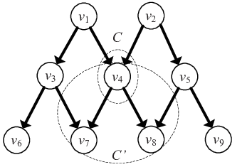
In Figure 1, for example, $C=\{v_{4}\}$ is a causal cut set, which separates the variables into the causal cut $\left(C=\{v_{4}\},V_{1}=\{v_{1},v_{3},v_{6},v_{7}\},V_{2}=\{v_{2},v_{5},v_{8},v_{9}\}\right)$. Given a directed graph $G$, there could be different valid causal cut sets satisfying the above conditions. In the example graph, $C^{\prime}=\{v_{4},v_{7},v_{8}\}$ is another causal cut set with $V_{1}=\{v_{1},v_{3},v_{6}\}$ and $V_{2}=\{v_{2},v_{5},v_{9}\}$.

Please note that causal cut set is closely related to the concept of $d$-separation but it may not lead to $d$-separation. For example, in the causal cut $\left(C=\{v_{4}\},V_{1}=\{v_{1},v_{3},v_{6},v_{7}\},V_{2}=\{v_{2},v_{5},v_{8},v_{9}\}\right)$ , the variable $v_{7}$ is not independent of $v_{2}$ given any subset of the causal cut set $C=\{v_{4}\}$; while in the causal cut $\left(C^{\prime}=\{v_{4},v_{7},v_{8}\},V_{1}=\{v_{1},v_{3},v_{6}\},V_{2}=\{v_{2},v_{5},v_{9}\}\right)$, the causal cut set $C^{\prime}$ lead to the $d$-separation between $V_{1}$ and $V_{2}$. The connection between causal cut and $d$-separation will be formalized in the next section.

Given a causal cut $\left(C,V_{1},V_{2}\right)$ on variable set $V$, we are able to transfer the causation discovery problem on $V$ into two smaller ones over the variable sets $V_{1}\cup C$ and $V_{2}\cup C$ respectively. This partitioning operation could be recursively called, until the number of variables involved in the subproblem is below a specified threshold $\theta$. The complete pseudocodes are available in Algorithm 1. The inputs of SADA include the sample set $D$, the variables $V$, a threshold $\theta$ and an underlying causation discovery algorithm $A$. Here, $\theta$ is used to terminate the recursive partitioning when the variable set is sufficiently small, and $A$ is an arbitrary basic causal solver invoked to find the actual causal structure on the subset of variables. $A$ is usually taken as a basic causal solver in this work.

In the rest of the section, we will discuss how to effectively and efficiently find causal cut on a variable set $V$ by exploiting the corresponding observational samples. We will also present the details of the merging operator, which tackles the problem of inconsistency and redundancy on the partial results from the subproblems. Note that only the faithfulness condition and causal sufficiency assumption are employed in this proposed framework (except the basic causal solver), thus SADA can work with different basic causal solvers by exploiting additional data generation assumptions, such as linear non-Gaussian data, additive noise data and so on.

The searching of the causal cut is crucial to the partitioning operation in SADA. To identify potential causal cut, our algorithm resorts to conditional independence testing over variables in the Bayesian network. The following lemma formalizes the connection.

Note that Lemma 1 is a sufficient condition of causal cut, but not a necessary condition. That is, a causal cut $\left(C,V_{1},V_{2}\right)$ may not satisfy the above three conditions. For example, the triple $\left(C=\{v_{4}\},V_{1}=\{v_{1},v_{3},v_{6},v_{7}\},V_{2}=\{v_{2},v_{5},v_{8},v_{9}\}\right)$ is a causal cut of the example given in Figure 1, but it dose not satisfy the condition (3) of Lemma 1, because the variable $v_{7}$ is not independent of $v_{2}$ given any subset of the causal cut set $C=\{v_{4}\}$. In detail, when $C_{uv}=\emptyset$, $v_{7}$ is dependent on $v_{2}$ because of the directed path $v_{2}\rightarrow v_{4}\rightarrow v_{7}$; when $C_{uv}=\{v_{4}\}$, $v_{7}$ is dependent on $v_{2}$ because of the directed path $v_{2}\rightarrow v_{4}\leftarrow v_{1}\rightarrow v_{3}\rightarrow v_{7}$ ( the path $v_{2}\rightarrow v_{4}\leftarrow v_{1}$ is connected given the variable $v_{4}$).

By exploiting the sufficient condition given in Lemma 1, we derive a new algorithm to find a causal cut set $C$, and the corresponding causal cut $\left(C,V_{1},V_{2}\right)$. In the search algorithm, each variable is heuristically assigned to one of the set $V_{1}$, $V_{2}$ and $C$. Besides of casual cut property, we also want to optimize the following two objectives during the assignment procedure: (1)minimizing the size of $C$. Because $C$ appears in both subproblems $V_{1}\cup C$ and $V_{1}\cup C$, i.e., smaller $C$ is preferred; (2) minimizing the size difference of $V_{1}$ and $V_{2}$. According to the principle of divide-and-conquer, the causal cut with similar sizes of $V_{1}$ and $V_{2}$ is preferred.

The details of the algorithms are listed in Algorithm 2. The algorithm runs with $k$ different initial variable pairs. The algorithm greedily adds the variable $w$ into $V_{1}$ (or $V_{2}$), if $w$ is independent of all the variables of $V_{2}$ (or $V_{1}$) given some subset of $C$. Only the $w$ can not added to neither of $V_{1}$ and $V_{2}$, $w$ is added to $C$. After completing all assignments, the algorithm also tries to move the variables from $C$ to $V_{1}$ or $V_{2}$ to maximize the partitioning effect. Finally, the causal cut with largest $\min\{|V_{1}|,|V_{2}|\}$ are returned as final result. We leave the discussion on the parameters $k$ and $\theta$ to next section. Please note that the sample size needed in the cut algorithm highly depends on the local connectivity of the causal structure but not on the number of variables. This is an important advantage of the algorithm to applications in large scale sparse causation discovery problems.

Given the example structure of Figure 1, the running step is given in Table I under the assumption that $V_{1}$, $V_{2}$ and $C$ are initialized as $\{v_{1}\}$ , $\{v_{2}\}$ and $\emptyset$, respectively. Among the steps, $v_{3}$ and $v_{6}$ are marginally independent of any variable of the current $V_{2}$. In another word, $C^{\prime}=\emptyset$ is used in the conditional independence test. The similar cases happen in the assignment of $v_{5}$ and $v_{9}$. In the checking of $v_{7}$, $v_{7}$ is dependent of the variables of $v_{2}$ given any sub set of the current causal cut set $C=\{v_{4}\}$ and added to the causal cut set $C$. $v_{8}$ is processed similarly.

As is shown in Algorithm 1, two partial results $G_{1}$ and $G_{2}$ are combined as a single casual graph as on variables in $V$. Since $G_{1}$ and $G_{2}$ are calculated independently but contain overlap over the causal cut set $C$. Thus conflict and redundancy need to be carefully handled in the merging operation. Recall the example given in Figure 1, assume $C=\{v_{4},v_{7},v_{8}\}$, $V_{1}=\{v_{1},v_{3},v_{4},v_{6},v_{7}\}$ and $V_{2}=\{v_{2},v_{4},v_{5},v_{8},v_{8},v_{9}\}$, the edges $v_{7}\rightarrow v_{8}$ and $v_{8}\rightarrow v_{7}$ may be appear in results from $V_{1}$ and $V_{2}$, generating conflicts. Similarly, the basic solver may return $v_{4}\rightarrow v_{7}$ and $v_{7}\rightarrow v_{8}$ on $V_{1}$, and $v_{4}\rightarrow v_{8}$ on $V_{2}$. It is easy to see, the edge $v_{7}\rightarrow v_{8}$ is redundant. Generally speaking, such conflicts and redundancy depend on the assumption of the causal structures. Under the directed acyclic graph assumption, the examples shown in Fig 2 are all the patterns we can detect.

The general form of a conflict is a cycle of directed edges among a group of variables, as shown in Figure 2(a). Given two nodes $v_{1}$ and $v_{2}$, there are two paths co-existing, such as $v_{1}\rightarrow\cdots\rightarrow v_{2}$ and $v_{1}\leftarrow v_{2}$. These two paths form a cycle and violate the acyclic constraints. To resolve such conflict, we simply remove the least reliable edge in the cycle, whenever a cycle is found. Here the reliability of the edge $v_{1}\rightarrow v_{2}$ is measured by the significance level, $sig\left(v_{1}\rightarrow v_{2}\right)$, which is returned by the basic causal solvers. For example, the $p$-value of the Wald test is used as the significance level for edges returned by LiNGAM [3], and the $p$-value of the noise’s independence of the causal variable is used as the significance level for edges returned by additive noise model [34].

Figure 2(b) illuminates a potential redundancy case. Given two variables $v_{1}$ and $v_{2}$, if both $v_{1}\rightarrow\cdots\rightarrow v_{2}$ and $v_{1}\rightarrow v_{2}$ are discovered, $v_{1}\rightarrow v_{2}$ may be redundant. Because the dependency relation $v_{1}\rightarrow v_{2}$ could be blocked by certain variables in the variable set $Path\left(v_{1}\rightarrow v_{2}\right)$. Here, $Path\left(v_{1}\rightarrow v_{2}\right)$ refers to the variable set involved in the directed path $v_{1}\rightarrow\cdots\rightarrow v_{2}$. Such redundancy raises when the following two conditions are satisfied: (1) the source and destination variables are both in the causal cut set, i.e., $v_{1},v_{2}\in C$, (2) there is another variable set $V_{3}\subset V_{1}$ (or $V_{3}\subset V_{2}$), such that $v_{1}\rightarrow V_{3}\rightarrow v_{2}$. If the above two conditions are met, one path $v_{1}\rightarrow v_{2}$ will be returned from the subproblem over $V_{1}\cup C$, while another path $v_{1}\rightarrow v_{2}$ turns up from the other subproblem over $V_{2}\cup C$. To tackle this problem, our merging algorithm runs the following conditional independence tests to verify if $\exists V^{\prime}\subset Path\left(v_{1}\rightarrow v_{2}\right)$ that $v_{1}\bot v_{2}|V^{\prime}$.

To summarize, the merging operation works as follows. Firstly, all directed edges from both solutions are simply added into a single edge set. Secondly, edges are ranked according to the associated significance measure, calculated by the basic causal solver employed by SADA. Thirdly, a sequential conflict testings are run over the ordered edges non-decreasingly on the significance. An edge is removed if it is conflicted with any of the previous edges. Finally, the redundancy edges are discovered and removed based on results of the conditional independence tests. A complete description is available in Algorithm 3.

In this part of the section, we aim to verify the effectiveness of the causal cut finding algorithm. In particular, we try to prove that the scale of the subproblem is significantly reduced by applying the randomized causal cut finding algorithm.

The last theorem implies that the causal cut finding algorithm is effective on reducing the scale of the subproblems. Another implication is on the selection of the parameter $\theta$. To guarantee there is a reduction on problem size, the parameter $\theta$ should be no smaller than $2d_{m}+2$, since such $\theta$ ensuring that $\frac{\theta}{2d_{m}+2}\geq 1$.

The accuracy of the causation discovery is measured based on the recall and precision on the result causal edges, i.e., the percentage of accurate causal edges and the percentage of causal edges returned. In this section, we show that SADA always finds fully accurate results in terms of recall and precision, if the invoked basic causal solver and conditional independence tests are both reliable.

Basically, the theorem above claims that the recall and precision on the causal edges returned by SADA are always satisfiable. However, as we emphasized at the beginning of the section, the assumption on reliable conditional independence tests is impractical, since randomness and noises always exist in the samples. In next section, we relax the assumption and show that SADA remains effective in a class of much more general settings.

Causal cut benefits SADA algorithm by improving the recall and precision of the basic causal solver when applied on sub-problems with much smaller scale. The side effect of the causal cut is the additional error overhead caused by undetected causal variable pairs which are separated in the causal cut. In this part of the section, we aim to give an analysis on the expectation of the causal cutting error in the partitioning step of SADA. To simplify the analysis, instead of using the original randomized causal cut finding algorithm, we uniformly divides the variables into $V_{1}$, $C$ and $V_{2}$, given the specific sizes $n_{1}$, $n_{2}$, $n_{c}$. Note that such partitioning is unaware of the actual causal structure. The causal cutting error incurred by SADA algorithm is thus definitely smaller than the estimation.

We assume that $V_{1}$, $C$ and $V_{2}$ are random variable sets output by the uniform assignment. Based on the assumptions, it is equivalent to assign the causal edges into the graph, from a null causal structure on the fixed partitioning result $V_{1}$, $C$ and $V_{2}$. We thus derive all the probabilities by simulating the random edge assignment process as following.

Let $\Psi$ denote the set of all causal structures over the current variable set $V$, and $\Psi_{i}$ denote a subset of $\Psi$ with exactly $i$ edges between $V_{1}$ and $V_{2}$. Given Assumption 3, the probability of having an actual structure $\psi\in\Psi_{i}$ could be evaluated using Equation (1), as the edges are independently assigned to the variables in $V$ and there are $e$ actual causal edges and $f$ non-causal ordered pairs,

Intuitively, in the equation, $\frac{e}{f+e}$ denotes the probability that there is a direct edge between a particular pair of variables. Similarly, $\frac{f}{f+e}$ denotes the probability that there is no edge between a particular pair of variables.

Moreover, we can further evaluate the probability of generating a valid partitioning in terms of the algorithmic condition in SADA. Particularly, SADA does not accept a partitioning if it finds a potential causal edge between any $v_{1}\in V_{1}$ and $v_{2}\in V_{2}$. We thus derive Equation (2) below to evaluate the joint probability of $\psi\in\Psi_{i}$ and $\Lambda(V_{1},V_{2})$. $\Lambda(V_{1},V_{2})$ refers to the event that there is no causal edge across $V_{1}$ and $V_{2}$ detected by the conditional independence tests:

Given Equation (1) and Equation (2), we apply Bayesian rule to estimate the probability of generating a partition $\left(C,V_{1},V_{2}\right)$ by the causal cut finding algorithm, under the condition of $\Lambda(V_{1},V_{2})$, i.e.,

The expectation of the error $e_{ce}$ caused by the causal cut finding, i.e., the number of undetected edges across $V_{1}$ and $V_{2}$, could be calculated as

References

- [1] J. Pearl, Causality: models, reasoning and inference, 2nd ed. Cambridge Univ. Press, 2009.
- [2] P. Spirtes, C. Glymour, and R. Scheines, Causation, Prediction, and Search, 2nd ed. The MIT Press, 2001.
- [3] S. Shimizu, P. O. Hoyer, A. Hyvärinen, and A. J. Kerminen, “A linear non-Gaussian acyclic model for causal discovery,” Journal of Machine Learning Research, vol. 7, pp. 2003–2030, 2006.
- [4] S. Shimizu, T. Inazumi, Y. Sogawa, A. Hyvärinen, Y. Kawahara, T. Washio, P. O. Hoyer, and K. Bollen, “DirectLiNGAM: A direct method for learning a linear non-Gaussian structural equation model,” Journal of Machine Learning Research, vol. 12, pp. 1225–1248, 2011.
- [5] P. O. Hoyer, D. Janzing, J. Mooij, J. Peters, and B. Schölkopf, “Nonlinear causal discovery with additive noise models,” in NIPS, 2008, pp. 689–696.
- [6] J. Peters, D. Janzing, and B. Schölkopf, “Identifying cause and effect on discrete data using additive noise models,” in AIStats, 2010, pp. 597–604.
- [7] P. Daniusis, D. Janzing, J. Mooij, J. Zscheischler, B. Steudel, K. Zhang, and B. Schoelkopf, “Inferring deterministic causal relations,” in UAI, 2010, pp. 143–150.
- [8] C. Yoo and G. Cooper, “Discovery of gene-regulation pathways using local causal search.” in Proceedings of the AMIA Symposium. American Medical Informatics Association, 2002, pp. 914–918.
- [9] B. Ellis and W. H. Wong, “Learning causal bayesian network structures from experimental data,” Journal of the American Statistical Association, vol. 103, no. 482, pp. 778–789, 2008.
- [10] C. Aliferis, A. Statnikov, I. Tsamardinos, S. Mani, and X. Koutsoukos, “Local causal and Markov blanket induction for causal discovery and feature selection for classification,” Journal of Machine Learning Research, vol. 11, pp. 171–234, 2010.
- [11] M. Kalisch and P. Bühlmann, “Estimating high-dimensional directed acyclic graphs with the PC-algorithm,” The Journal of Machine Learning Research, vol. 8, pp. 613–636, 2007.
- [12] R. Cai, Z. Zhang, and Z. Hao, “BASSUM: A Bayesian semi-supervised method for classification feature selection,” Pattern Recognition, vol. 44, no. 4, pp. 811–820, 2011.
- [13] Z. Zhu, Y.-S. Ong, and M. Dash, “Markov blanket-embedded genetic algorithm for gene selection,” Pattern Recognition, vol. 40, no. 11, pp. 3236–3248, 2007.
- [14] J. Pearl and T. Verma, “A theory of inferred causation,” in Proceedings of the 2nd International Conference on Principles of Knowledge Representation and Reasoning, 1991, pp. 441–452.
- [15] R. Cai, Z. Zhang, and Z. Hao, “Causal gene identification using combinatorial v-structure search,” Neural Networks, vol. 43, pp. 63–71, 2013.
- [16] F. Bromberg and D. Margaritis, “Improving the reliability of causal discovery from small data sets using argumentation,” Journal of Machine Learning Research, vol. 10, pp. 301–340, 2009.
- [17] X. Xie and Z. Geng, “A recursive method for structural learning of directed acyclic graphs,” Journal of Machine Learning Research, vol. 9, pp. 459–483, 2008.
- [18] R. Yehezkel and B. Lerner, “Bayesian network structure learning by recursive autonomy identification,” Journal of Machine Learning Research, vol. 10, pp. 1527–1570, 2009.
- [19] Y. He and Z. Geng, “Active learning of causal networks with intervention experiments and optimal designs.” Journal of Machine Learning Research, vol. 9, no. 11, 2008.
- [20] K. Zhang and A. Hyvärinen, “On the identifiability of the post-nonlinear causal model,” in UAI, 2009, pp. 647–655.
- [21] D. Janzing, J. Mooij, K. Zhang, J. Lemeire, J. Zscheischler, P. Daniusis, B. Steudel, and B. Schölkopf, “Information-geometric approach to inferring causal directions,” Artificial Intelligence, vol. 182-183, pp. 1–31, 2012.
- [22] Z. Chen, K. Zhang, L. Chan, and B. Schölkopf, “Causal discovery via reproducing kernel hilbert space embeddings,” Neural Computation, 2014.
- [23] B. Steudel, D. Janzing, and B. Schölkopf, “Causal Markov condition for submodular information measures,” in COLT, 6 2010, pp. 464–476.
- [24] D. Janzing and B. Schölkopf, “Causal inference using the algorithmic markov condition,” IEEE Transcation on Information Theory, vol. 56, no. 10, pp. 5168–5194, Oct. 2010.
- [25] T. Tashiro, S. Shimizu, A. Hyvärinen, and T. Washio, “Parcelingam: A causal ordering method robust against latent confounders,” Neural computation, vol. 26, no. 1, pp. 57–83, 2014.
- [26] J. Mooij, D. Janzing, J. Peters, and B. Schölkopf, “Regression by dependence minimization and its application to causal inference in additive noise models,” in ICML, 2009, pp. 745–752.
- [27] K. Zhang, J. Peters, D. Janzing, and B. Schölkopf, “Kernel-based conditional independence test and application in causal discovery,” in UAI, 2011.
- [28] J. Peters, J. Mooij, D. Janzing, and B. Schölkopf, “Identifiability of causal graphs using functional models,” in UAI, 2011, pp. 589–598.
- [29] C. Granger, “Investigating causal relations by econometric models and cross-spectral methods,” Econometrica, vol. 37, pp. 424–438, 1969.
- [30] S. Hacker and A. Hatemi, “Tests for causality between integrated variables using asymptotic and bootstrap distributions: theory and application,” Applied Economics, vol. 38, no. 13, pp. 1489–1500, 2006.
- [31] N. Mukhopadhyay and S. Chatterjee, “Causality and pathway search in microarray time series experiment,” Bioinformatics, vol. 23, no. 4, p. 442, 2007.
- [32] A. C. Lozano, N. Abe, Y. Liu, and S. Rosset, “Grouped graphical Granger modeling for gene expression regulatory networks discovery,” Bioinformatics, vol. 25, no. 12, pp. i110–i118, 2009.
- [33] D. Koller and N. Friedman, Probabilistic Graphical Model: Principles and Techniques, 2nd ed. The MIT Press, 2009.
- [34] J. Peters, D. Janzing, and B. Schölkopf, “Causal inference on discrete data using additive noise models,” IEEE Transactions on Pattern Analysis and Machine Intelligence, vol. 33, no. 12, pp. 2436 – 2450, 2011.
- [35] K. Zhang, H. Peng, L. Chan, and A. Hyvärinen, “Ica with sparse connections: Revisited,” in International Conference on Independent Component Analysis and Signal Separation. Springer, 2009, pp. 195–202.
- [36] K. Baba, R. Shibata, and M. Sibuya, “Partial correlation and conditional correlation as measures of conditional independence,” Australian & New Zealand Journal of Statistics, vol. 46, no. 4, pp. 657–664, 2004.