Higher order derivative coupling to gravity and its cosmological implications
Abstract
We show that the operator in effective field theory is significant for avoiding the instability of nonsingular bounce, where and are the three-dimensional Ricci scalar and the extrinsic curvature on the spacelike hypersurface, respectively. We point out that the covariant Lagrangian of , i.e., , has the second order derivative couplings of scalar field to gravity which do not appear in Horndeski theory or its extensions, but does not bring the Ostrogradski ghost. We also discuss the possible effect of on the primordial scalar perturbation in inflation scenario.
I Introduction
Recently, the studies of the origin of the universe and the current accelerated expansion have greatly promoted the development of gravity theories beyond general relativity (GR), see [1][2][3] for recent reviews. How to design a theory without extra degree of freedom (DOF) has acquired persistent attention.
The Horndeski theory was proposed in the 1970s [4], see also [5][6], in which the equations of motion have at most second order time derivatives, which avoids the extra DOF (so the Ostrogradski ghost). However, it seems that equations of motion with higher order time derivatives do not necessarily suggest the presence of extra DOF. The discoveries of the beyond Horndeski theory [7][8][9] and degenerate higher order scalar tensor (DHOST) theory [10][11][12][13] have confirmed this possibility and greatly enriched our understanding of gravity. In Horndeski and DHOST theories, the Lagrangian involves only the nonminimal couplings and , where , and .
Along a different line, the effective field theory (EFT) of cosmological perturbations has been developed for investigating inflation [14][15] and current cosmological acceleration [16][17][18], see [19] for a review. Recently, the EFT has also been applied to the nonsingular cosmologies [20][21][22]. It was found first in Refs. [20][21] that the operators with three-dimensional Ricci scalar , especially , could play a significant role in curing the gradient instability induced by a negative sound speed squared (i.e., ) of scalar perturbation [23][24]. Actually, as will be shown, the operator ( is the extrinsic curvature) could play a role similar to that of .
We built a fully stable cosmological bounce scenario in Ref. [25] by applying a least set of operators ( and ), namely, a “least modification”. The graviton throughout the bounce behaves itself like that in GR, which could naturally avoid the strong coupling regime appearing in [26], see also [27]. The covariant Lagrangian proposed in [25] belongs to beyond Horndeski theory, (see also [28] for a different implementation of a fully stable bounce), which is a subclass of the DHOST theory, but the equations of motion still could be second order in time derivatives. This enlightens us that there might still be some space of scalar-tensor theory to be explored.
As will be pointed out, the covariant description of contains the second order derivative couplings of the field to gravity, such as , and , which do not appear in Horndeski (or even DHOST) theory. The mimetic gravity with the coupling has been proposed in Ref. [29]. In scalar-tensor theory, it is interesting to explore the possibility of such higher order derivative couplings.
In this paper, we point out that the covariant Lagrangian of , i.e., , has the second order derivative couplings of scalar field to gravity which do not appear in Horndeski theory or its extensions but does not bring the Ostrogradski ghost. We discuss its implication on scalar-tensor theory. We also show the interesting applications of in the nonsingular cosmologies and the inflation scenario.
II Higher order derivative coupling to gravity
As was first found in [20] (see also [21]), the operator plays a crucial role in solving the gradient instability problem induced by , (see also [30] for the unitarity problem), which suffered by the nonsingular cosmologies based on the Horndeski theory [23][24][31][32]. In the Appendix, we point out that the operator actually could play a role similar to that of . As will be shown, the covariant Lagrangian of contains the second order derivative of coupled to gravity, such as , and . However, in Horndeski theory, such derivative couplings do not appear, since they will bring the Ostrogradski ghost. Thus, it is interesting to have a survey.
In this section, we will derive the covariant Lagrangian of in unitary gauge. The induced metric on the three-dimensional spacelike hypersurface () is , where is the unit vector orthogonal to the hypersurface and , with and . The extrinsic curvature is defined as
| (1) |
Since , it is straightforward to get
| (2) |
with . In unitary gauge , we have . Using the Gauss-Codazzi relation, we have
| (3) | |||||
Note that in the second line of Eq. (3), we also have with , as given in Ref. [25].
We define , with
| (4) | |||||
where the leading contribution of is the perturbation at quadratic order, so that could be a function of , (and even and ), and . When is set, reduces to .
Recalling that in Horndeski theory, contains the coupling of the second order derivative of to gravity, i.e., (or ). Here, we require that is also dependent, otherwise will be equivalent to , the cosmological applications of which have been studied, see, e.g., [33][34][35][36]. While in , the couplings
| (5) | |||||
| (6) |
appear, which are independent with . In addition, such couplings to gravity also include , , which are not independent and could be obtained by the combinations of and (5), as pointed out in Ref. [12].
In Horndeski theory, the cubic order of in will induce the higher derivatives in the metric and field equations, which are actually set off by [37]. This makes it be free from the Ostrogradski ghost. In DHOST theory [10][11], all possible terms of cubic order of the second order derivative of appear, which result in higher order equations of motion, but there is still no Ostrogradski ghost due to the degeneracy.
Though the DHOST theory extends the Horndeski theory, the coupling of the second order derivative of to gravity is still only , since the derivative couplings (5) and (6) will bring the Ostrogradski ghost (higher derivatives in the equations of motion). However, in , the Ostrogradski ghost could be dispelled by the combination of , , etc., and , see (4).
In principle, we could merge the Horndeski (even DHOST) theory and into a (second order) derivative coupling theory with all independent couplings (, (5) and (6)) of the second order derivative of to gravity. In such a theory, the background equations of motion could be set only by the Horndeski (DHOST) theory, since only contributes at leading order.
The quadratic coupling of the second order derivative of to , such as , might be obtained in or equivalently , where all coefficients must be fixed as (4).
In mimetic gravity [38][39] (see e.g., [40] for a review), since , instead of , the operator might be significant for curing the instabilities pointed out in [41][42][43]. Here, since the mimetic constraint suggests , we have
| (7) |
the covariant will be simpler.
It should be mentioned that at quadratic order also contributes , which is harmful or harmless, depending on the coefficient. However, could be removed by using (if required), since at leading order. We define and , with
| (8) | |||||
where both -order and the coupling of to actually appear and is a function of and (and even and ). In addition, itself also has an interesting application in nonsingular cosmologies [20][44].
III Cosmological applications
III.1 Stable model for ekpyrotic scenario
We consider the ekpyrotic scenario [45][46]. How to build a fully stable bounce model is a significant issue. We proposed such a model with in Ref. [25]. In Ref. [28], Kolevatov et al. also proposed a different model by applying the “inverse method” adopted in [23][47]. However, with the covariant , the design is actually simpler [25]. Here, with , the method is similar (though slightly complicated).
We begin with the ekpyrotic Lagrangian
| (9) | |||||
| Contraction and expansion | |||||
| Removing ghost |
with constant . must be satisfied around , so that . In [25], see also [48][49], we adopted
| (10) |
with the constants (switching the sign before in (9) around ), and (making appear around ). A full ekpyrotic Lagrangian (9) also should involve a mechanism (a coupling [50][51][52]) responsible for the scale invariant primordial perturbation.
The quadratic action of scalar perturbation for (9) is
| (11) |
where
| (12) |
and ; see the Appendix (or Ref. [20]) for details. In the Appendix, we have , and . The quadratic action of tensor perturbation is unaffected by and is still that in GR.
Here, we require , so that can be obtained. If , around the bounce point , we will have . However, since and satisfies
| (13) |
we always could set with suitable . It should be mentioned that when , crosses 0.
III.2 Slow-roll inflation with modified
We consider the inflation scenario. Here, the covariant and also only affect the sound speed of scalar perturbation, but the background and the tensor perturbation are unaffected. The effect of modified may be encoded in the power spectrum of primordial scalar perturbation, which might be observable.
The Lagrangian is
| (15) |
where is responsible for the inflation. We set the slow-roll parameter for simplicity. The quadratic action of scalar perturbation is given in (23) of the Appendix with . We have and
| (16) |
| (17) |
Here, modifies . We require , which suggests that in (17) is determined by and .
The equation of motion for is
| (18) |
with the definition and , and the superscript ′ is the derivative with respect to . The initial state of the perturbation mode is . The power spectrum of is
| (19) |
We have for slow-roll inflation (). Here, if is required, in (16) should be satisfied. This will result in , since while . Thus, the case with might be interesting.
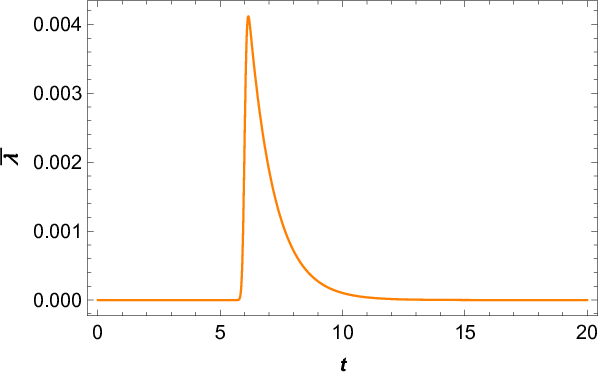
For an example, we consider a model in which acquires a dip (Fig.1(a)). We numerically show the corresponding evolutions of and in Figs. 1(b) and 1(c), according to (16) and (17), which could be rewritten as and since . We plot in Fig.1 (d) by solving Eq.(18), see [53][54][55] for a similar method. We see that the effect of on could be encoded in the power spectrum of scalar perturbation.
The phenomenological effect of is very similar to that of at quadratic order, if the contribution of to term in the quadratic action is totally canceled by , i.e., , which requires with . However, when the condition is violated, Eq. (18) should be modified to where (for simplicity, we will focus on the cases in which initially so that the initial state of the perturbation mode is still ).
Phenomenologically, we could distinguish the operator from . First, when , the frequency of the oscillations in the power spectrum will increase with , while the frequency of the oscillations is nearly constant for , see Fig. 2(b). Second, when (even when slightly deviates from ), may induce a larger amplitude of oscillations than that of in the power spectrum, as numerically shown in Fig. 2, unless has more drastic (or fine-tuned) variation.
The effect of varying on scalar perturbations has been also studied in Refs. [56][57][58][59][60][61], but based on (or equivalent EFT).




IV Discussion
Recently, it has been found in [20][21] that the operators with three-dimensional Ricci scalar in EFT, especially , are significant for solving the problem of , which is suffered by the nonsingular cosmologies. Here, we find that the operator actually could play a role similar to that of .
We derived the covariant Lagrangian of . The covariant has the second order derivative coupling of the field to gravity, such as (5) and (6) (which do not appear in Horndeski and DHOST theory), but does not bring the Ostrogradski ghost. This suggests that the Horndeski (or even DHOST) theory and might be merged into a second order derivative coupling theory with all possible independent couplings, i.e., (or ), (5) and (6), of the second order derivative of to gravity. Here, how (5) and (6) consistently appear in such a theory is just what is told by the covariant description of the operator.
With , we built a fully stable cosmological model for the ekpyrotic scenario, by applying similar method used in Ref. [25]. Our work indicates that with the covariant (proposed in [25]) or , the stable nonsingular bounce scenario could be concisely designed. Here, our study is motivated straightly by the EFT operators, e.g., [20]. However, other studies based on modified gravity will also be interesting [62, 63, 64, 65, 66, 67, 68], especially their stabilities.
We also studied the possible effect of on the primordial scalar perturbation in the inflation scenario, which might be encoded in the TT spectrum of cosmic microwave background (CMB). We will come back to the relevant issues elsewhere.
Acknowledgments
We thank Yunlong Zheng, Mingzhe Li and Xian Gao for helpful discussions. YC would like to thank Youping Wan and Yi-Fu Cai for discussions and hospitality during his visit at University of Science and Technology of China. This work is supported by NSFC, No. 11575188, 11690021, and also supported by the Strategic Priority Research Program of CAS, No. XDA04075000, XDB23010100.
Appendix A The EFT
As pointed out in Refs. [47][22], the cubic Galileon only moves the period of to the outside of the null energy condition (NEC) violating phase but cannot dispel it completely, see also the earlier discussion [69] on this point.
In this Appendix, we briefly review the EFT for nonsingular cosmologies, and show how the and operators play crucial roles in solving the problem of .
With the ADM line element, we have
| (20) |
and , where . The induced metric on three-dimensional hypersurface is , where , is orthogonal to the spacelike hypersurface, and . Thus,
| (21) |
The EFT action is
| (22) | |||||
where , is the three-dimensional Ricci scalar, is the extrinsic curvature and . The first row describes the background, while the rest are for the perturbations. We always could set , which implies and . See, e.g., [20] for the details.
Here, we only consider the coefficients set and set other coefficients in (22) equal to 0. Only with , the quadratic action of scalar perturbation is (see, e.g., our [20])
| (23) |
where
| (24) | |||
| (25) | |||
| (26) | |||
| (27) | |||
| (28) |
Only if and is the nonsingular cosmological model healthy. In models with the operator , can be obtained, since contributes , while can be avoided since or contributes .
References
- [1] V. A. Rubakov, Phys. Usp. 57, 128 (2014) [Usp. Fiz. Nauk 184, 2, 137 (2014)] [arXiv:1401.4024 [hep-th]].
- [2] A. Joyce, B. Jain, J. Khoury and M. Trodden, Phys. Rept. 568, 1 (2015) [arXiv:1407.0059 [astro-ph.CO]].
- [3] S. Nojiri, S. D. Odintsov and V. K. Oikonomou, arXiv:1705.11098 [gr-qc].
- [4] G. W. Horndeski, Int. J. Theor. Phys. 10, 363 (1974).
- [5] C. Deffayet, X. Gao, D. A. Steer and G. Zahariade, Phys. Rev. D 84, 064039 (2011) [arXiv:1103.3260 [hep-th]].
- [6] T. Kobayashi, M. Yamaguchi and J. Yokoyama, Prog. Theor. Phys. 126, 511 (2011) [arXiv:1105.5723 [hep-th]].
- [7] M. Zumalacárregui and J. García-Bellido, Phys. Rev. D 89, 064046 (2014) [arXiv:1308.4685 [gr-qc]].
- [8] J. Gleyzes, D. Langlois, F. Piazza and F. Vernizzi, Phys. Rev. Lett. 114, 21, 211101 (2015) [arXiv:1404.6495 [hep-th]].
- [9] J. Gleyzes, D. Langlois, F. Piazza and F. Vernizzi, JCAP 1502, 018 (2015) [arXiv:1408.1952 [astro-ph.CO]].
- [10] D. Langlois and K. Noui, JCAP 1602, 02, 034 (2016) [arXiv:1510.06930 [gr-qc]].
- [11] D. Langlois and K. Noui, JCAP 1607, 07, 016 (2016) [arXiv:1512.06820 [gr-qc]].
- [12] J. Ben Achour, M. Crisostomi, K. Koyama, D. Langlois, K. Noui and G. Tasinato, JHEP 1612, 100 (2016) [arXiv:1608.08135 [hep-th]].
- [13] D. Langlois, M. Mancarella, K. Noui and F. Vernizzi, JCAP 1705, 05, 033 (2017) [arXiv:1703.03797 [hep-th]].
- [14] C. Cheung, P. Creminelli, A. L. Fitzpatrick, J. Kaplan and L. Senatore, JHEP 0803, 014 (2008) [arXiv:0709.0293 [hep-th]].
- [15] S. Weinberg, Phys. Rev. D 77, 123541 (2008) [arXiv:0804.4291 [hep-th]].
- [16] G. Gubitosi, F. Piazza and F. Vernizzi, JCAP 1302, 032 (2013) [arXiv:1210.0201 [hep-th]].
- [17] J. Gleyzes, D. Langlois, F. Piazza and F. Vernizzi, JCAP 1308, 025 (2013) [arXiv:1304.4840 [hep-th]].
- [18] F. Piazza and F. Vernizzi, Class. Quant. Grav. 30, 214007 (2013) [arXiv:1307.4350 [hep-th]].
- [19] A. Naskar, S. Choudhury, A. Banerjee and S. Pal, arXiv:1706.08051 [astro-ph.CO].
- [20] Y. Cai, Y. Wan, H. G. Li, T. Qiu and Y. S. Piao, JHEP 1701, 090 (2017) [arXiv:1610.03400 [gr-qc]].
- [21] P. Creminelli, D. Pirtskhalava, L. Santoni and E. Trincherini, JCAP 1611, 11, 047 (2016) [arXiv:1610.04207 [hep-th]].
- [22] Y. Cai, H. G. Li, T. Qiu and Y. S. Piao, Eur. Phys. J. C 77, 6, 369 (2017) [arXiv:1701.04330 [gr-qc]].
- [23] M. Libanov, S. Mironov and V. Rubakov, JCAP 1608, 08, 037 (2016) [arXiv:1605.05992 [hep-th]].
- [24] T. Kobayashi, Phys. Rev. D 94, 4, 043511 (2016) [arXiv:1606.05831 [hep-th]].
- [25] Y. Cai and Y. S. Piao, arXiv:1705.03401 [gr-qc].
- [26] A. Ijjas and P. J. Steinhardt, Phys. Lett. B 764, 289 (2017) [arXiv:1609.01253 [gr-qc]].
- [27] D. Yoshida, J. Quintin, M. Yamaguchi and R. H. Brandenberger, arXiv:1704.04184 [hep-th].
- [28] R. Kolevatov, S. Mironov, N. Sukhov and V. Volkova, arXiv:1705.06626 [hep-th].
- [29] Y. Zheng, L. Shen, Y. Mou and M. Li, arXiv:1704.06834 [gr-qc].
- [30] C. de Rham and S. Melville, Phys. Rev. D 95, no. 12, 123523 (2017) [arXiv:1703.00025 [hep-th]].
- [31] R. Kolevatov and S. Mironov, Phys. Rev. D 94, 12, 123516 (2016) [arXiv:1607.04099 [hep-th]].
- [32] S. Akama and T. Kobayashi, Phys. Rev. D 95, 6, 064011 (2017) [arXiv:1701.02926 [hep-th]].
- [33] K. Feng, T. Qiu and Y. S. Piao, Phys. Lett. B 729, 99 (2014) [arXiv:1307.7864 [hep-th]].
- [34] H. Mohseni Sadjadi and P. Goodarzi, Phys. Lett. B 732, 278 (2014) [arXiv:1309.2932 [astro-ph.CO]].
- [35] N. Yang, Q. Fei, Q. Gao and Y. Gong, Class. Quant. Grav. 33, 20, 205001 (2016) [arXiv:1504.05839 [gr-qc]]; Y. Zhu and Y. Gong, Int. J. Mod. Phys. D 26, 02, 1750005 (2016) [arXiv:1512.05555 [gr-qc]].
- [36] T. Harko, F. S. N. Lobo, E. N. Saridakis and M. Tsoukalas, Phys. Rev. D 95, 4, 044019 (2017) [arXiv:1609.01503 [gr-qc]]; J. B. Dent, S. Dutta, E. N. Saridakis and J. Q. Xia, JCAP 1311, 058 (2013) [arXiv:1309.4746 [astro-ph.CO]].
- [37] C. Deffayet, S. Deser and G. Esposito-Farese, Phys. Rev. D 80, 064015 (2009) [arXiv:0906.1967 [gr-qc]].
- [38] A. H. Chamseddine, V. Mukhanov and A. Vikman, JCAP 1406, 017 (2014) [arXiv:1403.3961 [astro-ph.CO]].
- [39] A. H. Chamseddine and V. Mukhanov, JCAP 1703, 03, 009 (2017) [arXiv:1612.05860 [gr-qc]].
- [40] L. Sebastiani, S. Vagnozzi and R. Myrzakulov, Adv. High Energy Phys. 2017, 3156915 (2017) [arXiv:1612.08661 [gr-qc]].
- [41] A. Ijjas, J. Ripley and P. J. Steinhardt, Phys. Lett. B 760, 132 (2016) [arXiv:1604.08586 [gr-qc]].
- [42] H. Firouzjahi, M. A. Gorji and A. Hosseini Mansoori, arXiv:1703.02923 [hep-th].
- [43] S. Hirano, S. Nishi and T. Kobayashi, arXiv:1704.06031 [gr-qc].
- [44] Y. Misonoh, M. Fukushima and S. Miyashita, Phys. Rev. D 95, 4, 044044 (2017) [arXiv:1612.09077 [gr-qc]].
- [45] J. Khoury, B. A. Ovrut, P. J. Steinhardt and N. Turok, Phys. Rev. D 64, 123522 (2001) [hep-th/0103239].
- [46] J. L. Lehners, Phys. Rept. 465, 223 (2008) [arXiv:0806.1245 [astro-ph]].
- [47] A. Ijjas and P. J. Steinhardt, Phys. Rev. Lett. 117, 12, 121304 (2016) [arXiv:1606.08880 [gr-qc]].
- [48] M. Koehn, J. L. Lehners and B. Ovrut, Phys. Rev. D 93, 10, 103501 (2016) [arXiv:1512.03807 [hep-th]].
- [49] M. Koehn, J. L. Lehners and B. A. Ovrut, Phys. Rev. D 90, 2, 025005 (2014) [arXiv:1310.7577 [hep-th]].
- [50] M. Li, Phys. Lett. B 724, 192 (2013) [arXiv:1306.0191 [hep-th]].
- [51] A. Fertig, J. L. Lehners and E. Mallwitz, Phys. Rev. D 89, 10, 103537 (2014) [arXiv:1310.8133 [hep-th]].
- [52] A. Ijjas, J. L. Lehners and P. J. Steinhardt, Phys. Rev. D 89, 12, 123520 (2014) [arXiv:1404.1265 [astro-ph.CO]].
- [53] Y. Cai, Y. T. Wang and Y. S. Piao, Phys. Rev. D 93, 6, 063005 (2016) [arXiv:1510.08716 [astro-ph.CO]].
- [54] Y. Cai, Y. T. Wang and Y. S. Piao, Phys. Rev. D 91, 103001 (2015) [arXiv:1501.06345 [astro-ph.CO]].
- [55] Y. Cai, Y. T. Wang and Y. S. Piao, JHEP 1602 (2016) 059 [arXiv:1508.07114 [hep-th]].
- [56] M. Nakashima, R. Saito, Y. i. Takamizu and J. Yokoyama, Prog. Theor. Phys. 125, 1035 (2011) [arXiv:1009.4394 [astro-ph.CO]].
- [57] M. Park and L. Sorbo, Phys. Rev. D 85, 083520 (2012) [arXiv:1201.2903 [astro-ph.CO]].
- [58] N. Bartolo, D. Cannone and S. Matarrese, JCAP 1310, 038 (2013) [arXiv:1307.3483 [astro-ph.CO]].
- [59] A. Achucarro, V. Atal, B. Hu, P. Ortiz and J. Torrado, Phys. Rev. D 90 (2014) 2, 023511 [arXiv:1404.7522 [astro-ph.CO]].
- [60] R. Saito and Y. i. Takamizu, JCAP 1306, 031 (2013) [arXiv:1303.3839 [astro-ph.CO]].
- [61] S. Mizuno, R. Saito and D. Langlois, JCAP 1411, no. 11, 032 (2014) [arXiv:1405.4257 [hep-th]].
- [62] S. Banerjee and E. N. Saridakis, Phys. Rev. D 95, 6, 063523 (2017) [arXiv:1604.06932 [gr-qc]].
- [63] T. Biswas, E. Gerwick, T. Koivisto and A. Mazumdar, Phys. Rev. Lett. 108, 031101 (2012) [arXiv:1110.5249 [gr-qc]]; T. Biswas, A. S. Koshelev, A. Mazumdar and S. Y. Vernov, JCAP 1208, 024 (2012) [arXiv:1206.6374 [astro-ph.CO]].
- [64] M. Vasilic, Phys. Rev. D 95, 12, 123506 (2017) [arXiv:1704.02589 [gr-qc]].
- [65] Y. B. Li, J. Quintin, D. G. Wang and Y. F. Cai, JCAP 1703, 03, 031 (2017) [arXiv:1612.02036 [hep-th]].
- [66] S. D. Odintsov and V. K. Oikonomou, Phys. Rev. D 92 (2015) 2, 024016 [arXiv:1504.06866 [gr-qc]]; S. D. Odintsov and V. K. Oikonomou, Phys. Rev. D 91 (2015) 6, 064036 [arXiv:1502.06125 [gr-qc]]; S. D. Odintsov and V. K. Oikonomou, Phys. Rev. D 90 (2014) 12, 124083 [arXiv:1410.8183 [gr-qc]].
- [67] S. H. Hendi, M. Momennia, B. Eslam Panah and M. Faizal, Astrophys. J. 827, 2, 153 (2016) [arXiv:1703.00480 [gr-qc]]; S. H. Hendi, M. Momennia, B. Eslam Panah and S. Panahiyan, Phys. Dark Universe 16, 26 (2017) [arXiv:1705.01099 [gr-qc]].
- [68] M. Giovannini, Phys. Rev. D 95, 8, 083506 (2017) [arXiv:1612.00346 [hep-th]].
- [69] D. A. Easson, I. Sawicki and A. Vikman, JCAP 1111, 021 (2011) [arXiv:1109.1047 [hep-th]].