Recently, several discrepancies with the standard model (SM) have been revealed in $b\to s\ell^{+}\ell^{-}$ induced decays, e.g., [1]. However, those that do not involve lepton flavor universality violation are not definitely settled due to poorly controlled non-perturbative effects of quantum chromodynamics (QCD). Exemplary, non-factorizable corrections to form factors are commonly considered as one unreducible uncertainty while interpreting beyond the standard model (BSM) physics. Furthermore, in $c\to u\ell^{+}\ell^{-}$ transitions, non-factorizable corrections yield the largest perturbative contribution due to the Glashow–Iliopolus–Maiani (GIM) cancellation of factorizable contributions [2, 3, 4]. In this paper, we improve on the current state by calculating the two loop virtual corrections to any heavy to light transition, including $c$ and $b$ decays, induced by current-current operators for arbitrary invariant dilepton mass $q^{2}$.

Partonic transitions are a first approximation to the corresponding inclusive hadronic decays in the framework of an operator product expansion (OPE). This approximation is applicable away from resonance regions and up to power corrections. The resonance regions can be handled by appropriate kinematical cuts and power corrections can be treated within a heavy quark expansion (an expansion in inverse powers of the heavy quark mass, see [5] for $b\to s$ transitions). Furthermore, perturbative results are the basis for estimates of non-perturbative effects in inclusive and exclusive hadronic decays, e.g., [6, 7].

Several calculations were performed for $b\to(d,s)$ transitions: In [8] and [9] $b\to s$ and $b\to d$ transitions, respectively, were computed for small $q^{2}$. The calculation of $b\to s$ transitions for large $q^{2}$ was accomplished in [10]. A seminumerical approach was employed in [5] to present results based on $b\to s$ transitions for the full $q^{2}$ range. In [11] $b\to d$ transitions for any $q^{2}$ range were computed, extending [9]. For $c\to u$ transitions, see [12]. We emphasize that available results for $b\to(d,s)$ transitions only cover different limits, i.e. zero masses, small and large $q^{2}$ ranges, and that results for $c\to u$ transitions have become available only recently [12, 4]. The analytic calculation presented in this paper covers the full $q^{2}$ range, arbitrary masses and electric charges.

Generally, the effective weak Lagrangian for heavy to light quark flavor changing neutral current (FCNC) transitions $h\to l$ at the low-energy scale $\mu$ is written as

where the sum is over light quark fields $q$ with masses below $\mu$, and products of Cabibbo–Kobayashi–Maskawa (CKM) matrix elements $\lambda_{q}=V_{q(d,s)}^{*}V_{qb},V_{cq}^{*}V_{uq}$ for $b\to(d,s)$ and $c\to u$ transitions, respectively. Here, $C_{i}$ are the Wilson coefficients and the physical operators $P_{i}$, which are relevant for this paper, read

where $q_{L/R}=\tfrac{1}{2}(1\mp\gamma_{5})q$, $\sigma^{\mu_{1}\mu_{2}}=\tfrac{i}{2}[\gamma^{\mu_{1}},\gamma^{\mu_{2}}]$, and $T^{a}$ are the $SU(3)_{C}$ generators normalized to $\mathrm{Tr}[T^{a}T^{b}]=\tfrac{\delta^{ab}}{2}$. Furthermore, $G_{F}$ is the Fermi constant, $F_{\mu_{1}\mu_{2}}$ denotes the electromagnetic field strength tensor, and $g_{s}$ and $e$ are the strong and electromagnetic coupling constants, respectively.

We calculate the two loop QCD matrix elements of $P_{1/2}$, in terms of form factors (i.e., for inclusive decays, effective Wilson coefficients) multiplying the matrix elements of $P_{7,9}$, for $h\to l\ell^{+}\ell^{-}$ transitions. The result is valid for a general class of heavy to light transitions with arbitrary invariant momentum transfer and masses, when the mass of the light quark is neglected. This includes the transitions $b\to(d,s)$ via $(u\bar{u},c\bar{c})$ loops, and $c\to u$ via $(d\bar{d},s\bar{s})$ loops, where the loop quark-antiquark pair $(q\bar{q})$ is annihilated and a photon is emitted, which may then couple to a lepton pair. Note that the computation of two loop matrix elements presented in this paper is not restricted to SM applications, see [12] for an example in leptoquark models. We use the recent works [13] and [14] for the master integrals (MIs) and their numerical evaluation, respectively.

We outline our calculation in the section 2, see also [12]. The numerical evaluation is detailed in section 2.1. Results are given in section 3, where we also comment on the phenomenological impact for $b\to(d,s)$ transitions. For the phenomenology of $c\to u$ transitions, see [12]. Appendix A contains a description of supplemented files, which encode the results of this paper.

In this section, we outline the calculation of the diagrams shown in figure 1. Each of the five subsets represents a gauge invariant class. A sixth class, shown in figure 2, preserves the operator structure of $P_{9}$, hence it is commonly considered as a correction to the matrix element of $P_{9}$ [8] and not included in the calculation presented in this paper. Nevertheless, we have checked that in this class only the diagram with a photon coupling to the loop of the quark-antiquark pair is non-zero and factorizes into two one loop integrals. It is the only diagram with infrared and collinear singularities.

We calculate the diagrams in figure 1 with insertions of $P_{2}$. Insertions of $P_{1}$ are then given by color factors due to additional generators in the definition of the operator: The expressions for the first four and last (two) classes are multiplied with $\tfrac{-1}{6}$ and $\tfrac{4}{3}$, respectively.

The matrix element for an off-shell photon $\gamma^{*}$ can be decomposed as [11]

where $q^{\mu}=(p_{h}-p_{l})^{\mu}$ is the transferred momentum, and $X^{\mu}$ is the sum of the amputated diagrams in figure 1.

The scalar form factors $F^{(i)}$ are given as [11]

with the projectors

and coefficients $C_{ij}$. The factors $(\not{p}_{h}+m_{h})$ and $\not{p}_{l}$ reflect the on-shell conditions for the external quarks. The form factors for $\langle l\ell\ell|P_{2}|h\rangle$, thus the effective Wilson coefficients, are proportional to $F^{(7,9)}$. By gauge invariance, the form factor $F^{(q)}$ vanishes for each class, which we have checked.

For the calculation, we utilize the computer programs FORM 4.0 [15] and REDUZE 2 [16]. We use the former for algebraic manipulations, e.g. the tensor algebra, and the latter is used for the reduction to MIs. The program REDUZE 2 is based on the Laporta algorithm [17] which employs integration by parts (IBP) identities [18] and Lorentz invariance (LI) identities [19]. Indeed, LI identities can be written as linear combinations of IBP identities [20]. We have calculated relations for each diagram based on LI identities by hand and checked them against the reduction tables built with REDUZE 2.

We find that the following diagrams in figure 1 vanish: In the fifth class, both diagrams with photons attached to the external lines vanish. The diagram with a photon emitted from the heavy quark line in the first class is zero. For $F^{(7)}$, all diagrams with photons attached to the external lines vanish. Furthermore, all diagrams of the fifth class vanish for $F^{(7)}$. This implies that the $\langle P_{1}\rangle$ induced dipole form factor is given by $\tfrac{-1}{6}F^{(7)}$.

As for the set of the MIs, we match a subset of the integrals calculated in [13]. A canonical set is given in [10], where the MIs are calculated for large $q^{2}$, yet the set of integrals is not minimal. While matching the set of [10] onto the MIs taken from [13], we find additional relations among the former, e.g. for the integral $I_{d23}$ and the one of equation (A12) in [10]. Furthermore, we do not encounter the integrals of equations (A5), (A8), and (A14) in [10].

With the MIs from [13] the unrenormalized form factors are expressed in terms of (generalized) harmonic polylogarithms (HPLs), see the next section for the numerical evaluation. The prescription for the renormalization is described in, e.g., [8]. Accordingly, the operator renormalization constants are written as

where the dimension is $4-2\epsilon$. Extending the set of the physical operators $P_{i}$ by the evanescent operators $E_{11,12}$ defined as

the coefficients $a_{ij}$ are compactly written as

and

Here, $P_{4}=(\bar{l}_{L}\gamma_{\mu_{1}}T^{a}h_{L})\sum_{\{q:m_{q}<\mu\}}(\overline{q}\gamma^{\mu_{1}}T^{a}q)$, $n_{f}$ is the number of flavors and $q_{e,i}$ are the charges of the external and internal quarks, respectively, i.e. $q_{e}=\tfrac{-1}{3}$, $q_{i}=\tfrac{2}{3}$ for $b\to(d,s)$ and $q_{e}=\tfrac{2}{3}$, $q_{i}=\tfrac{-1}{3}$ for $c\to u$ transitions. The coefficients $a_{ij}^{11,22}$ can be obtained from the leading order (LO) anomalous dimension matrix (ADM) $\gamma^{(0)}$ and the coefficients $a_{ij}^{12}$ from [21],

where $\gamma^{(1)}$ is the next-to leading order (NLO) ADM, and the mixing via the evanescent operators is found as

The counterterm form factors $F_{i\to(7,9)}^{\text{ct}(7,9)}$, due to the mixing of $P_{1/2}$ into $P_{7,9}$, and the one loop renormalization of $g_{s}$ in the definition of $P_{9}$, are [8, 9]

where $\beta_{0}=11-\tfrac{2}{3}n_{f}$.

The counterterms $F_{i\to 4\text{quark}}^{\text{ct}(7,9)}$, due to the mixing of $P_{1/2}$ into four-quark operators $P_{j}$, are defined by [8]

We calculate them to $\mathcal{O}(\epsilon)$ and for insertions of $P_{1,2,4}$, $E_{11,12}$ according to eqs. (18) and (12), respectively. We write

where in the massless limit, $m_{q}^{2}\to 0$,

and the residual $m_{q}^{2}$ dependence cancels to $\mathcal{O}(\epsilon)$ in eq. (19). With this, the matrix elements are evaluated to

We have checked that expanding the matrix elements in small $q^{2}$ and in the limit $m_{q}^{2}\to 0$ yields the results in [8] and [11], respectively.

Following [8], the renormalization of the mass $m_{q}$ is given by the replacement $m_{q}\to Z_{m_{q}}m_{q}$ in $\langle l\ell\ell|P_{1,2}|h\rangle_{1\text{loop}}$ of eq. (21). The mass renormalization constants $Z_{m}$ in the modified minimal subtraction ($\overline{\text{MS}}\lx@text@overline{\text{MS}}$) and the pole mass scheme are [22]

Expanding the matrix elements at $\mathcal{O}(\tfrac{\alpha_{s}}{4\pi})$ and $\mathcal{O}(\epsilon^{0})$ gives the counterterms $F_{i,m_{q}}^{\text{ct}(9)}$ and $F_{i,m_{q}}^{\text{ct}(7)}=0$. We have checked for both schemes that expanding the counterterm $F_{i,m_{q}}^{(9)}$ in small $q^{2}$ yields the results in [8].

Factorizable form factors represented by class 5 in figure 1 are found to be renormalized separately by the mass renormalization and mixing into evanescent operators, i.e. $a^{11}_{2\,11}=\tfrac{1}{2}$ in eq. (12), and $a_{29}^{12}=\tfrac{4}{9}q_{i}$ in eq. (13) are the only non-zero coefficients for the counterterms of $F_{2}^{(9fac)}$; recall that the $\langle P_{1}\rangle$ induced factorized form factor is given by color factors and the dipole factorized form factors are zero.

Finally, the renormalized form factors are given by subtracting $F_{i}^{\text{ct}(7,9)}=(F_{i\to 7,9}^{\text{ct}(7,9)}+F_{i\to 4\text{quark}}^{\text{ct}(7,9)}+F_{i,m_{q}}^{\text{ct}(7,9)})$ from the unrenormalized form factors. Note that wave function renormalization of the external quark fields would need to be taken into account only if we wanted to include the diagrams of figure 2 [8]. We have checked that $F_{i}^{\text{ct}(7)}|_{\epsilon^{0}}$ agrees with the results in [5].

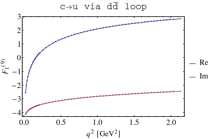
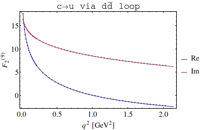
Our fitted results of the renormalized form factors $F_{1,2}^{(7,9)}$ induced by $\langle l\ell\ell|P_{1,2}|h\rangle$ for $b\to(d,s)$ and $c\to u$ transitions are shown in figures 3-6 for $q^{2}\in[0,m_{h}^{2}]$. For comparison, we also show the results of [8, 11, 10]. We use the (pole) masses

$m_{u,d}\approx 0$ and set $\mu=m_{h}$ if not stated otherwise.

We note the following:

• •

  The results of [8, 11, 10] agree well with our results, hence the former are only partially visible in the plots.

• •

  The form factors are divergent at the internal quark pair mass squared $q^{2}=(2m_{i})^{2}$.

• •

  The lower left plot of figure 3 indicates a numerical precision of our results better than ${10}^{-3}$ with respect to the analytical result of [11].

• •

  The lower right plot of figure 3 shows agreement with the expansion of [10] at high $q^{2}$. Note that we do not plot the ratio close to the kinematical endpoint $q^{2}=m_{b}^{2}$, where the evaluation of the result of [10] yields oscillations. At low $q^{2}$, a breakdown of the convergence of the expansion of [8] is visible around $q^{2}\sim$5\text{\,}\mathrm{G}\mathrm{e}\mathrm{V}$^{2}$, where the sensitivity on $\mu$ increases. Similar conclusions are drawn from figure 5.

Furthermore, note that our definition of the form factors and the one in [8, 10] differs by a minus sign. Recall that $F_{1}^{(7)}=\tfrac{-1}{6}F_{2}^{(7)}$. For $F_{1,2}^{(9)}$, the numerical precision of our results is better than ${10}^{-2}$ with respect to the results of [8, 11, 10] for $b\to(d,s)$ transitions.

We deduce that the overall numerical precision of our result is better than a percent. To have ready-to-use result at hand, we provide our results for the masses of eq. (23) as supplemented files, see appendix A.

Next, we comment on the impact of the new results for $b\to(d,s)$ transitions. For massless internal quarks an independent analytical result is provided in [11]. The high $q^{2}$ range for massive internal quarks is well approximated by the results of [10]. On the other side, compared to the low $q^{2}$ range [8] for massive internal quarks, our results indicate significant corrections around $q^{2}\sim$5\text{\,}\mathrm{G}\mathrm{e}\mathrm{V}$^{2}$. Following [5] and [10] for the matrix element of the chromomagnetic operator, the effective Wilson coefficients $\tilde{C}_{7,9}^{\text{eff}}$ at next-to-next-to leading logarithmic (NNLL) order are shown in figures 7, 8. We add our results and, for comparison, the results of [8] for $$1\text{\,}\mathrm{G}\mathrm{e}\mathrm{V}$^{2}\leq q^{2}\leq$7\text{\,}\mathrm{G}\mathrm{e}\mathrm{V}$^{2}$. Note that for phenomenological purposes $\tilde{P}_{7,9}=\tfrac{\alpha_{s}}{4\pi}P_{7,9}$, thus $\tilde{C}_{7,9}=\tfrac{4\pi}{\alpha_{s}}C_{7,9}$.

One observes that the real parts are stable, whereas corrections to imaginary parts increase to several percent towards higher $q^{2}$. The effective Wilson coefficients obey the hierarchies $\mathrm{Re}[\tilde{C}_{7,9}^{\text{eff}}]\gg\mathrm{Im}[\tilde{C}_{7,9}^{\text{eff}}]$. Thus, observables which only depend on the real parts or magnitudes of the effective Wilson coefficients are marginally affected by our results as long as the results of [8, 11, 10] are taken into account. On the other hand, effects on observables which depend on the imaginary parts of the effective Wilson coefficients are significant in the low $q^{2}$ range.

Our fitted results of the renormalized form factors $F_{2}^{(9fac)}$, class 5 in figure 1, are shown in figure 9 for $q^{2}\in[-m_{h}^{2},m_{h}^{2}]$.

We note that the factorized form factors are smooth below the internal quark pair threshold and real in the Euclidean region. One observes that for vanishing internal masses, see left plots in figure 9, the shapes only differ by the ratio of internal charges and $q^{2}$ scales with the ratio of external masses.

In this paper, we calculated the effective Wilson coefficients for heavy to light FCNC transitions induced by the matrix elements of current-current operators at two loop. The results are valid for arbitrary momentum transfer and masses, when the light mass is neglected. For the MIs, we used the works of [13, 14]. Our computation extends previous works on $b\to(d,s)\ell^{+}\ell^{-}$ transitions [8, 9, 11, 10] and is new for $c\to u\ell^{+}\ell^{-}$ transitions. We found significant corrections to the imaginary parts of the effective Wilson coefficients for $b\to(d,s)$ transitions in the large hadronic recoil range, see figure 8, which should be included in future analyses, including BSM studies. Other corrections for $b\to(d,s)$ transitions were found to be marginal. For $c\to u$ transitions and an application to leptoquark models, we refer to [12]. Along with this paper we provide supplemented files, containing our analytical results and fitted results for a specific set of parameters. Finally, our calculation is an independent check of the results of [13, 14] and [8, 9, 11, 10], with which we agree in the corresponding limits.

We acknowledge Tobias Huber for several useful discussions. We thank Christoph Bobeth and Gudrun Hiller for useful comments on the manuscript. This work has been supported in part by the DFG Research Unit FOR 1873 “Quark Flavour Physics and Effective Field Theories”.

References

- [1] T. Blake et al. “Round table: Flavour anomalies in processes” In Proceedings, 12th Conference on Quark Confinement and the Hadron Spectrum (Confinement XII): Thessaloniki, Greece 137, 2017, pp. 01001 DOI: 10.1051/epjconf/201713701001
- [2] Christoph Greub, Tobias Hurth, Mikolaj Misiak and Daniel Wyler “The contribution to weak radiative charm decay” In Phys. Lett. B382, 1996, pp. 415–420 DOI: 10.1016/0370-2693(96)00694-6
- [3] Stefan de Boer and Gudrun Hiller “Flavor and new physics opportunities with rare charm decays into leptons” In Phys. Rev. D93.7, 2016, pp. 074001 DOI: 10.1103/PhysRevD.93.074001
- [4] Thorsten Feldmann, Bastian Mueller and Dirk Seidel “ Decays in the QCD Factorization Approach” In JHEP 08, 2017, pp. 105 DOI: 10.1007/JHEP08(2017)105
- [5] A. Ghinculov, T. Hurth, G. Isidori and Y.. Yao “The Rare decay to NNLL precision for arbitrary dilepton invariant mass” In Nucl. Phys. B685, 2004, pp. 351–392 DOI: 10.1016/j.nuclphysb.2004.02.028
- [6] Michael Benzke, Seung. Lee, Matthias Neubert and Gil Paz “Factorization at Subleading Power and Irreducible Uncertainties in Decay” In JHEP 08, 2010, pp. 099 DOI: 10.1007/JHEP08(2010)099
- [7] A. Khodjamirian, Th. Mannel, A.. Pivovarov and Y.-M. Wang “Charm-loop effect in and ” In JHEP 09, 2010, pp. 089 DOI: 10.1007/JHEP09(2010)089
- [8] H.. Asatryan, H.. Asatrian, C. Greub and M. Walker “Calculation of two loop virtual corrections to in the standard model” In Phys. Rev. D65, 2002, pp. 074004 DOI: 10.1103/PhysRevD.65.074004
- [9] H.. Asatrian, K. Bieri, C. Greub and M. Walker “Virtual corrections and bremsstrahlung corrections to in the standard model” In Phys. Rev. D69, 2004, pp. 074007 DOI: 10.1103/PhysRevD.69.074007
- [10] Christoph Greub, Volker Pilipp and Christof Schupbach “Analytic calculation of two-loop QCD corrections to in the high region” In JHEP 12, 2008, pp. 040 DOI: 10.1088/1126-6708/2008/12/040
- [11] Dirk Seidel “Analytic two loop virtual corrections to ” In Phys. Rev. D70, 2004, pp. 094038 DOI: 10.1103/PhysRevD.70.094038
- [12] Stefan de Boer “Probing the standard model with rare charm decays” http://hdl.handle.net/2003/36043, 2017
- [13] Guido Bell and Tobias Huber “Master integrals for the two-loop penguin contribution in non-leptonic B-decays” In JHEP 12, 2014, pp. 129 DOI: 10.1007/JHEP12(2014)129
- [14] Hjalte Frellesvig, Damiano Tommasini and Christopher Wever “On the reduction of generalized polylogarithms to and and on the evaluation thereof” In JHEP 03, 2016, pp. 189 DOI: 10.1007/JHEP03(2016)189
- [15] J. Kuipers, T. Ueda, J… Vermaseren and J. Vollinga “FORM version 4.0” In Comput. Phys. Commun. 184, 2013, pp. 1453–1467 DOI: 10.1016/j.cpc.2012.12.028
- [16] A. von Manteuffel and C. Studerus “Reduze 2 - Distributed Feynman Integral Reduction”, 2012 arXiv:1201.4330 [hep-ph]
- [17] S. Laporta “High precision calculation of multiloop Feynman integrals by difference equations” In Int. J. Mod. Phys. A15, 2000, pp. 5087–5159 DOI: 10.1016/S0217-751X(00)00215-7, 10.1142/S0217751X00002157
- [18] K.. Chetyrkin and F.. Tkachov “Integration by Parts: The Algorithm to Calculate beta Functions in 4 Loops” In Nucl. Phys. B192, 1981, pp. 159–204 DOI: 10.1016/0550-3213(81)90199-1
- [19] T. Gehrmann and E. Remiddi “Differential equations for two loop four point functions” In Nucl. Phys. B580, 2000, pp. 485–518 DOI: 10.1016/S0550-3213(00)00223-6
- [20] R.. Lee “Group structure of the integration-by-part identities and its application to the reduction of multiloop integrals” In JHEP 07, 2008, pp. 031 DOI: 10.1088/1126-6708/2008/07/031
- [21] Konstantin. Chetyrkin, Mikolaj Misiak and Manfred Munz “ nonleptonic effective Hamiltonian in a simpler scheme” In Nucl. Phys. B520, 1998, pp. 279–297 DOI: 10.1016/S0550-3213(98)00131-X
- [22] Christoph Bobeth, Mikolaj Misiak and Jorg Urban “Photonic penguins at two loops and dependence of ” In Nucl. Phys. B574, 2000, pp. 291–330 DOI: 10.1016/S0550-3213(00)00007-9
- [23] Jens Vollinga and Stefan Weinzierl “Numerical evaluation of multiple polylogarithms” In Comput. Phys. Commun. 167, 2005, pp. 177 DOI: 10.1016/j.cpc.2004.12.009
- [24] Sebastian Kirchner “LiSK - A C++ Library for Evaluating Classical Polylogarithms and ”, 2016 arXiv:1605.09571 [hep-ph]
- [25] Daniel Maitre “Extension of HPL to complex arguments” In Comput. Phys. Commun. 183, 2012, pp. 846 DOI: 10.1016/j.cpc.2011.11.015
- [26] Tobias Huber and Daniel Maitre “HypExp 2, Expanding Hypergeometric Functions about Half-Integer Parameters” In Comput. Phys. Commun. 178, 2008, pp. 755–776 DOI: 10.1016/j.cpc.2007.12.008