\dates

Compiled August 24, 2026 \ociscodes(090.0090) Holography; (090.1760) Computer holography; (090.2900) Optical storage materials.

Deep-learning-based data page classification for holographic memory

Journal: aoDOI: http://dx.doi.org/10.1364/ao.XX.XXXXXX

Tomoyoshi Shimobaba Affiliation: Graduate School of Engineering, Chiba University, 1-33 Yayoi-cho, Inage-ku, Chiba, 263-8522, Japan Affiliation: Corresponding author: shimobaba@faculty.chiba-u.jp Naoki Kuwata Affiliation: Graduate School of Engineering, Chiba University, 1-33 Yayoi-cho, Inage-ku, Chiba, 263-8522, Japan Mizuha Homma Affiliation: Department of Electrical and Electronics Engineering, Chiba University, 1-33 Yayoi-cho, Inage-ku, Chiba, 263-8522, Japan Takayuki Takahashi Affiliation: Graduate School of Engineering, Chiba University, 1-33 Yayoi-cho, Inage-ku, Chiba, 263-8522, Japan Yuki Nagahama Affiliation: Graduate School of Engineering, Chiba University, 1-33 Yayoi-cho, Inage-ku, Chiba, 263-8522, Japan Marie Sano Affiliation: Graduate School of Engineering, Chiba University, 1-33 Yayoi-cho, Inage-ku, Chiba, 263-8522, Japan Satoki Hasegawa Affiliation: Graduate School of Engineering, Chiba University, 1-33 Yayoi-cho, Inage-ku, Chiba, 263-8522, Japan Ryuji Hirayama Affiliation: Graduate School of Engineering, Chiba University, 1-33 Yayoi-cho, Inage-ku, Chiba, 263-8522, Japan Takashi Kakue Affiliation: Graduate School of Engineering, Chiba University, 1-33 Yayoi-cho, Inage-ku, Chiba, 263-8522, Japan Atsushi Shiraki Affiliation: Institute of Management and Information Technologies, Chiba University, 1-33 Yayoi-cho, Inage-ku, Chiba, 263-8522, Japan Naoki Takada Affiliation: Science Department, Natural Sciences Cluster, Research and Education Faculty, Kochi University, Kochi 780-8520, Japan Tomoyoshi Ito Affiliation: Graduate School of Engineering, Chiba University, 1-33 Yayoi-cho, Inage-ku, Chiba, 263-8522, Japan

Abstract

We propose a deep-learning-based classification of data pages used in holographic memory. We numerically investigated the classification performance of a conventional multi-layer perceptron (MLP) and a deep neural network, under the condition that reconstructed page data are contaminated by some noise and are randomly laterally shifted. The MLP was found to have a classification accuracy of 91.58%, whereas the deep neural network was able to classify data pages at an accuracy of 99.98%. The accuracy of the deep neural network is two orders of magnitude better than the MLP.

1 Introduction

Optical memories such as compact discs (CD), digital versatile discs (DVD) and Blu-ray discs utilize laser spots to read and write digital data. The recording disk is irradiated with the laser spot, condensed by a lens. Increasing the memory capacity requires miniaturization of the laser spot. In Blu-ray discs, the minimum spot is approximately 0.15 $\mu$ m. To achieve higher density, it is necessary to use a laser with a shorter wavelength and a lens with a higher numerical aperture, but it is coming to its limit.

In holographic memory [1, 2], digital data is converted into a two-dimensional pattern called a data page, and this is recorded on a recording medium as a hologram. The main features of the holographic memory are below: (1) the access speed is fast because the data page can be read and written as two-dimensional images, and (2) multiple data pages can be stored in the same recording area by multiplex recording characteristics of holography, leading to an increase in the memory capacity. In addition, the combination of holographic memory and optical encryption is interesting because the increased security, does not come at the expense of increased encryption and decryption time [3] .

Although holographic memory has a significant advantage as the next-generation data storage, problems do exist, such as bit errors arising from pixel misalignment and noise. Simple thresholding to a data page detected by an image sensor induces bit errors; therefore, we need sophisticated methods to correctly detect bits. Precise pixel alignment between reconstructed data pages and an imaging device are required to correctly read data pages. Solutions to this issue have been proposed [4]. Some noises (speckle noise, interpixel interference, interpage interference [2]) contaminate reconstructed data page. Solutions to the noises have been proposed, such as a Viterbi algorithm [5], a deconvolution method [6], a gradient decent method [7] and an autoencoder [8]. In addition, data pages coded via modulation and error-correction codes help in significantly improving bit errors when compared to raw data pages [9].

In this study, we propose a deep-learning-based classification of data pages. The deep neural network (convolutional neural network [10]) is learned, which is composed of convolutional layers, pooling layer, and a fully-connected layers, using data pages reconstructed from holograms, and then the learned deep neural network classified data pages. It is significant that the deep neural network can automatically acquire optimum data page classifications from learning datasets without human intervention.

We numerically investigated the classification performance between a conventional multi-layer perceptron (MLP) and the deep neural network. Under the condition that reconstructed data pages are contaminated by some noise and are randomly laterally shifted, the MLP had a classification accuracy of only 91.58%, whereas the deep neural network was able to classify the data pages at an accuracy of 99.98%.

2 Deep-learning-based classification for holographic memory

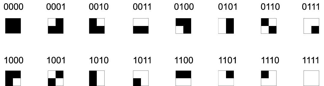
Figure 1 shows the deep-learning-base classification for holographic memory, where data pages are recorded as holograms. These data pages are composed of 4-bit patterns as shown in Fig.2. In this paper, we do not use multiple recording of data pages in the same region of the hologram, or modulation codes such as 6:8 modulation code, or error-correction codes. Imaging devices such as charge coupled devices (CCDs) and complementary MOS (CMOS) cameras captured the reconstructed data pages, which are contaminated by noise, from the holograms. The reconstructed data pages are divided into fragments corresponding to 4-bit original data. The deep neural network in which we used a convolutional neural network (CNN) classifies fragments into the most similar 4-bit pattern.

Refer to caption — Figure 1: Deep learning-based classification for holographic memory.

2.1 Hologram generation

In this study, we used amplitude holograms $I({\bm{m}})$ that are generated from data pages. The amplitude holograms are generated by

I({\bm{m}})=|O({\bm{m}})+R({\bm{m}})|^{2},

(1)

where ${\bm{m}}$ denotes a two-dimensional position vector in the hologram plane, $O({\bm{m}})$ is the object light of data pages that are displayed on a spatial light modulator, and $R({\bm{m}})$ is the reference light. The object light is obtained from the original data page, $u({\bm{n}})$ , using

O({\bm{m}})=\mathcal{{\rm Prop}}_{z}\bigl[u({\bm{n}}))\bigl],

(2)

where $\mathcal{{\rm Prop}}_{z}\bigl[\cdot\bigl]$ denotes the diffraction operator with a propagation distance of $z$ . ${\bm{n}}$ denotes a two-dimensional position vector in the object plane. The reconstructed data pages, $u^{\prime}(\bm{n})$ , from the holograms are obtained by

u`(\bm{n})=|\mathcal{{\rm Prop}}_{-z}\bigl[I(\bm{m})\bigl]|^{2}.

(3)

In this study, $R({\bm{m}})$ is the inline planar wave, so that the mathematical expression is simply $R({\bm{m}})=1$ . Thus, the reconstructed data pages were degraded by direct light and conjugate light.

2.2 Convolutional neural network

Figure 3 shows a CNN for classifying fragments of data pages. The CNN consists of convolution layers, pooling layers, and an MLP composed of fully connected layers and an output layer.

A convolution layer automatically acquires feature maps of input two-dimensional (2D) data $x_{ij}$ , where the subscript $ij$ denote the pixel index, using $M$ filters whose filter coefficients denote $h^{(m)}_{pq}$ where $m\in[0,M-1]$ . When setting $M$ different filters, the convolution layer acquire $M$ different feature maps. The output of the layer $y^{(m)}_{ij}$ is calculated by

y^{(m)}_{ij}=f\left(\sum_{p=0}^{H}\sum_{q=0}^{H}h^{(m)}_{pq}x_{ij}+b_{ij}\right)

(4)

where $f(\cdot)$ is an activate function, $H$ is the filter size and $b_{ij}$ is a bias. We used Leaky ReLU function ( $f(x)=x$ when $x>0$ ; otherwise, $f(x)=0.01x$ ) as the activate function because we confirmed that the classification performance of the activate function was better than that of the ReLU function for our situation. We used $H=5$ in the first convolutional layer filter and $H=3$ in the second convolutional layer.

A pooling layer had the effect of reducing the sensitivity of lateral movement of the input data. In addition, this layer was used for reducing the input data size, resulting in a decrease of the computational complexity. Several pooling layers have been proposed. The max pooling layer that we used was calculated by

y_{ij}={\rm max}\{x_{ij}\}.

(5)

Here, this layer divides the input 2D data $x_{ij}$ with $W\times W$ pixels into sub 2D images, and the maximum values in the sub images are selected and are used to generate the output image $y_{ij}$ with $W/2\times W/2$ pixels.

The MLP classifies fragments into the most similar 4-bit patterns, as shown in Fig.2. The structure of the MLP is shown in Fig.4. A fully connected layer in the MLP was calculated by

y_{j}=f\left(\sum_{i=1}^{U}w_{ji}x_{i}+b_{j}\right),

(6)

where $f(\cdot)$ is an activate function, $U$ is the number of units, $x_{i}$ is the input data, $w_{ji}$ is the weight coefficients, $y_{j}$ is the output data, and $b_{j}$ is a bias.

In the first and second fully connected layers, we used $U=128$ and the ReLU function as the activate function. The output layer calculates probabilities of classification using the softmax function, expressed as

y_{j}=\frac{\exp(x_{j})}{\sum_{i=1}^{U}\exp(x_{i})},

(7)

where $U=16$ because we wanted to classify the 16 fragments shown in Fig.2.

In the learning process of the CNN, we needed to prepare a large number of datasets composed of reconstructed fragments and corresponding correct answers. Using these datasets, we optimized the parameters (the filter coefficients $h^{(m)}_{pq}$ , weight coefficients $w_{ji}$ , and biases) in the CNN. These parameters were optimized by minimizing a cost function. In this study, we used the cross-entropy cost function, and, we used Adam [11], which is a stochastic gradient descent (SGD) method, as the optimizer, to minimize the cross-entropy cost function. This SGD randomly selects $B$ datasets among all of the datasets. $B$ is referred to as the batch size, and here, we used a batch size of 100. In addition, we used the Dropout method [12] to prevent overfitting in the CNN. Dropout randomly disables $d$ percent of units during the training process. We used $d=0.25$ % in the pooling layers and $d=0.5$ % in the fully connected layers.

3 Results

We compared the classification performance between the CNN, show in Fig.3, and a conventional MLP, shown in Fig.4.

The data pages and holographic reconstructions had $1,000\times 1,000$ pixels, and the fragments had $20\times 20$ pixels. The on-bit (1) and off-bit (0) in a fragment were both expressed by $10\times 10$ pixels. Thus, the number of fragments per one data page and holographic reconstruction was 2,500.

We prepared 375,000 fragments (150 data pages $\times$ 2,500 fragments) and their holographic reconstructions for the training of the CNN and MLP. For the testing of the CNN and MLP, we used another 125,000 fragments (50 data pages $\times$ 2,500 fragments) and their holographic reconstructions. The condition for the hologram calculation were are a wavelength of 633nm and sampling pitches of the holograms and reconstructions of 4 $\mu$ m. We used the angular spectrum method for the diffraction calculation.

We verified the classification performance of the CNN and the conventional MLP when changing the propagation distance $z$ in the hologram generation. Figure 5 shows a part of the reconstructed data pages when changing the propagation distance $z$ . We used $z$ =0.05, 0.1 and 0.15 m. As seen, the reconstructed data pages became blurred as the propagation distance increased, resulting in increased difficulty in the classification at the longer distance. In addition, we added the Gaussian noise with a mean of 0 and a standard variation of 2.5 to the intensity of the reconstructed data pages to verify the robustness against intensity noise. We added a random lateral shift of $\pm 5$ pixels to the reconstructed data pages to verify the robustness against the misalignment between the reconstructed data pages and the image sensor.

Table 1 shows the accuracy of the classification of the MLP and CNN when changing the propagation distance. Generally, for the accuracy metrics, in general, a bit error rate (BER) is used in holographic memory; however, we used a fragment error rate (FER) instead of the BER because the MLP and CNN classify the fragments. The FER was calculated by ${\rm FER}=N_{e}/N_{t}$ , where $N_{e}$ is the number of error fragments and $N_{t}$ is the number of total fragments in the test process. The FER of the MLP was around $10^{-2}$ , except at $z=$ 0.15m, whereas the FER of the CNN was around $10^{-4}$ , except at $z=$ 0.15 m, even if the propagation distance was changed. The CNN has an accuracy two orders of magnitude better than the MLP.

All calculations were done by deep-learning framework [13] and our wave optics library [14].

Table 1: Fragment error rate (FER) when changing the propagation distance.

	Fragment error rate
z (m)	MLP	CNN (proposal)
0.05	$8.42\times 10^{-2}$	$1.52\times 10^{-4}$
0.1	$5.07\times 10^{-2}$	$5.84\times 10^{-4}$
0.15	$1.88\times 10^{-1}$	$2.45\times 10^{-2}$

4 Conclusion

We proposed a CNN-based data page classification for holographic memory and compared the classification performance between a conventional MLP and a CNN. Even if the reconstructed data pages were contaminated by some noise and were randomly laterally shifted, the CNN could classify the data pages in fragment error rates of around $10^{-4}$ . It is significant that the deep neural network can automatically acquire optimum data page classification from learning data without human intervention. In this study, we used raw data pages without any modulation codes or error-correction codes. If we use these codes in the CNN, we expect to increase the classification performance. In our upcoming project, we plan to verify the CNN performance with these coding methods in a more realistic environment simulation [15].

Funding

This work was partially supported by JSPS KAKENHI Grant Numbers 16K00151.

References

[1] D. Psaltis, Demetri, and G. W. Burr, “Holographic data storage,” Computer 31, 52-60 (1998).
[2] H. Ruan, “Recent advances in holographic data storage,” Frontiers of Optoelectronics 7 450-466 (2014).
[3] O. Matoba, and B. Javidi, “Encrypted optical storage with angular multiplexing,” Appl. Opt. 38 7288-7293 (1999).
[4] G. W. Burr and T. Weiss, “Compensation for pixel misregistration in volume holographic data storage,” Opt. Lett. 26, 542-544 (2001).
[5] J. F. Heanue, K. Gürkan, and L. Hesselink, “Signal detection for page-access optical memories with intersymbol interference,” Appl. Opt. 35, 2431-2438 (1996).
[6] S-. H. Lee, S-. Y. Lim, N. Kim, N-. C. Park, H. Yang, K-. S. Park, and Y-.P. Park, “Increasing the storage density of a page-based holographic data storage system by image upscaling using the PSF of the Nyquist aperture,” Opt. Express 19, 12053-12065 (2011).
[7] D. H. Kim, S. Jeon, N. C. Park, and K. S. Park, “Iterative design method for an image filter to improve the bit error rate in holographic data storage systems,” Microsyst. Technol. 20, 1661-1669 (2014).
[8] T. Shimobaba, Y. Endo, R. Hirayama, Y. Nagahama, T. Takahashi, T. Nishitsuji, T. Kakue, A. Shiraki, N. Takada, N. Masuda, and T. Ito, “Autoencoder-based holographic image restoration,” Appl. Opt. 56, F27-F30 (2017).
[9] G. W. Burr, J. Ashley, H. Coufal, R. K. Grygier, J. A. Hoffnagle, C. M. Jefferson, and B. Marcus, “Modulation coding for pixel-matched holographic data storage,” Opt. Lett. 22, 639-641 (1997).
[10] A. Krizhevsky, I. Sutskever, and G. E. Hinton, “Imagenet classification with deep convolutional neural networks,” In Advances in neural information processing systems, 1097-1105 (2012).
[11] D. Kingma and B. Jimmy, “Adam: A method for stochastic optimization,” arXiv preprint arXiv:1412.6980 (2014).
[12] N. Srivastava, G. E. Hinton, A. Krizhevsky, I. Sutskever, and R. Salakhutdinov, “Dropout: a simple way to prevent neural networks from overfitting,” J. Mach. Learn. Res. 15, 1929-1958 (2014).
[13] https://github.com/fchollet/keras
[14] T. Shimobaba, J. Weng, T. Sakurai, N. Okada, T. Nishitsuji, N. Takada, A. Shiraki, N. Masuda, and T. Ito, “Computational wave optics library for C++: CWO++ library,” Comput. Phys. Commun. 183, 1124–1138 (2012).
[15] N. Kinoshita, H. Shino, N. Ishii, N. Shimizu, and K. Kamido, “Integrated simulation for volume holographic memory using finite-difference time-domain method,” Jpn. J. Appl. Phys. 44, 3503-3507 (2005).